Abstract
In this work, we propose an algorithm for the detection, measurement and classification of discontinuities in signals captured with noise. Our approach is based on the Harten’s subcell-resolution approximation adapted to the presence of noise. This technique has several advantages over other algorithms. The first is that there is a theory that allows us to ensure that discontinuities will be detected as long as we choose a sufficiently small discretization parameter size. The second is that we can consider different types of discretizations such as point values or cell-averages. In this work, we will consider the latter, as it is better adapted to functions with small oscillations, such as those caused by noise, and also allows us to find not only the discontinuities of the function, jumps in functions or edges in images, but also those of the derivative, corners. This also constitutes an advantage over classical procedures that only focus on jumps or edges. We present an application related to heart rate measurements used in sport as a physical indicator. With our algorithm, we are able to identify the different phases of exercise (rest, activation, effort and recovery) based on heart rate measurements. This information can be used to determine the rotation timing of players during a game, identifying when they are in a rest phase. Moreover, over time, we can obtain information to monitor the athlete’s physical progression based on the slope size between zones. Finally, we should mention that regions where heart rate measurements are abnormal indicate a possible cardiac anomaly.
Keywords:
corner and jump discontinuities; noise; ENO and subcell-resolution approximations; heart rate measurements; phases of exercise MSC:
65D15; 65Z05; 65T60
1. Introduction
Detecting discontinuities in functions plays a crucial role in various scientific, engineering, and computational applications. A discontinuity, a sudden and abrupt change in a function’s behavior, often signifies a significant transition or event. Understanding and identifying these points of disruption are essential for several reasons. In signal processing, identifying discontinuities helps separate meaningful information from noise. Detecting sudden changes in signal characteristics can be critical for accurate analysis. Discontinuity detection is fundamental in image processing for edge detection and segmentation. Recognizing abrupt changes in pixel intensities aids in identifying object boundaries. In mathematical analysis, recognizing points of discontinuity is crucial for understanding the properties of a function. It provides insights into the behavior of a function across different regions. In numerical methods, identifying discontinuities is vital for ensuring the stability and accuracy of algorithms. Algorithms may need to adapt their behavior in the presence of discontinuities. Understanding and detecting sudden changes in system behavior are essential for effective control systems. Identifying discontinuities helps in modeling and controlling dynamic systems. In data science, detecting abrupt changes in data sets is crucial for anomaly detection. Recognizing discontinuities aids in filtering out noise and identifying meaningful patterns. In computer vision applications, such as object recognition, detecting edges and contours relies on discontinuity detection. Recognizing sudden changes in visual data is fundamental for scene understanding. Discontinuity detection is essential in optimization problems where objective functions may have abrupt changes. Identifying these points helps optimization algorithms converge efficiently. In summary, the ability to detect and analyze discontinuities in functions is a fundamental aspect of various scientific and technological domains. It enhances our capability to interpret data, model systems, and develop algorithms that can adapt to different scenarios, ultimately contributing to advancements across a diverse range of fields.
Some of these processes produce piecewise smooth data, that is functions with a small number of discontinuities compared to the number of sampled data. Assume that the input function is corrupted by an additive random noise , we would like to find the discontinuities of the signal f. The noise disturbs the data thus the problem is complex. It is difficult to distinguish the true discontinuities from the function and the false discontinuities from the noise. The noise added to the signal appears as small oscillatory deviations from the curve.
In this work, we present an algorithm designed for the detection, measurement, and classification of signal discontinuities, particularly in the presence of noise. Our approach is rooted in Harten’s subcell-resolution approximation [1,2], which has been adapted to accommodate noisy signals.
For functions without noise, we can find other interesting approaches different from the Harten SR-technique. For instance, several recent findings have demonstrated the effectiveness of directional multiscale approaches, such as continuous curvelet and shearlet transforms, in providing a robust theoretical foundation for understanding the geometry of edge singularities [3]. These methods surpass the capabilities of traditional wavelet transforms. Specifically, the continuous shearlet transform offers a precise geometric characterization of edges in piecewise constant functions.
In [4], the authors expand upon previously known characterization results and demonstrate that, even for piecewise smooth functions, the continuous shearlet transform can identify the location and orientation of edge points, including corner points, by leveraging its asymptotic decay at fine scales. The new proof introduces innovative technical constructions to address this more challenging problem. These findings establish the theoretical groundwork for extending the application of the shearlet framework to a broader range of problems in image processing.
Certainly, various approaches have been introduced to approximate singularities in functions affected by noise. In this context, we revisited some of these methods, delving into their foundations and, more specifically, highlighting the motivation behind our approach due to several of its distinctive features. In [5], an image-denoising algorithm reliant on wavelets and multifractals for singularity detection was presented. The algorithm calculates the pointwise singularity strength value, characterizing local singularity at each scale. Through thresholding the singularity strength, wavelet coefficients are classified into edge-related and regular coefficients, and irregular coefficients. The irregular coefficients undergo denoising using an approximate minimum mean-squared error estimation method, while the edge-related and regular wavelet coefficients are smoothed using the fuzzy-weighted mean filter. This strategy aims to preserve edges and details during noise reduction. In [6], cubic box spline wavelets are presented, which have compact support and avoid phase shifts. It defines associated digital filters for the discrete dyadic wavelet transform, crucial for detecting and measuring signal singularities. The approach distinguishes between regular and irregular coefficients, enabling effective noise reduction while preserving edges and details.
Many other approaches propose edge detector algorithms for image-processing applications [7,8,9]. These approaches are based in heuristic ideas exhibiting good numerical behaviors but lacking a theoretical framework. See also the review paper [10] for an interesting application of edges detectors: fingerprint classification.
The Harten SR-approximation is supported by a nice theory [11] that ensures that we are able to find the singularities taking the discretization parameter smaller than a critical value depending only on the regularity of the function.
Our algorithm offers several advantages over the above methods. Firstly, it is underpinned by a theoretical foundation that ensures the detection of discontinuities, provided the discretization size of the function is chosen to be sufficiently small. Secondly, our approach allows for the consideration of various discretization types, including point values or averages in cells. For this work, we opt for the latter, as it is better suited for functions with minor oscillations, such as those induced by noise. Additionally, it enables the identification of not only the function’s discontinuities, jumps in functions or edges in images, but also those in its derivative, such as corners. This flexibility distinguishes our algorithm from classical procedures that primarily focus on jumps or edges.
We showcase a practical application related to heart rate measurements in sports as a physical indicator. Our algorithm proves effective in discerning different phases of exercise, such as rest, activation, effort, and recovery, based on heart rate measurements. It facilitates the determination of players’ rotation timing during a game by identifying rest phases. Furthermore, over time, the algorithm provides monitoring and insights into an athlete’s physical progression via based on the slope size between zones. Notably, our algorithm can pinpoint regions where heart rate measurements exceed typical records, indicating a potential cardiac anomaly. Finally, the detection is automatic and occurs in real time, two fundamental aspects for the coach team.
The remainder of the paper is organized as follows. In Section 2, preliminary information necessary to understand the algorithm is given. Next, the full detector mechanism is presented, followed by an examination of some academic examples to check the algorithms. Lastly, an application related to heart rate measurements applied in collective sport are presented, and concluding remarks are provided.
2. The Cell-Average Framework and the ENO-SR Approximation
Let us consider a set of nested grids in :
where is some fixed integer and we consider the discretization
where is the space of absolutely integrable functions in .
We now define the sequence in the k-th cell as:
If is the antiderivative of , then the sequence corresponds to a point-value discretization of in the k-th cell.
Now, we denote by an interpolation such that . Thus, we can obtain an approximation, , to using Equation (1):
From , it is obtained
Then, we can use an interpolation procedure for F to obtain a reconstruction for the original function f. We continue recalling the ENO interpolation strategy.
2.1. ENO Interpolation Strategy
The fundamental concept behind the ENO approach involves expanding the region of high accuracy by constructing piecewise polynomial interpolants that solely rely on information from smooth regions of the interpolated function.
Let be an uniform mesh and . Let and , where . Let be a polynomial interpolator of in X.
If we consider an interpolation of order r, we have
where is a polynomial of degree such that and . The set of r nodes associated to the polynomial forms a stencil, , associated to the interval . The nodes and have to be in .
The idea of the ENO interpolation is to construct a stencil using information of only from smooth parts. These techniques aim to minimize inaccuracies in reconstruction, particularly in regions with isolated singularities. Note that interpolation techniques relying on a predetermined stencil selection result in polynomial interpolants, that are merely first-order approximations to when their stencil crosses a singularity . Consequently, the accuracy of the piecewise polynomial interpolant diminishes over a substantial region around the singularity, with the extent of this effect depending on the degree of the polynomial pieces (i.e., the number of points in the stencil).
For each interval , we consider all possible stencils of cardinality that include the nodes and :
The task is to select, from all candidates, the one that meets our requirements. Let be the index corresponding to the second point of the selected stencil. Note that if , and no selection is necessary. Let us assume then that . The symbol represents the divided differences of the function H. In [2], Harten describes two possible procedures:
Note that if , then , , in both cases Algorithms 1 and 2.
Now, we recall the subcell resolution technique.
| Algorithm 1: Hierarchical Selection |
| Algorithm 2: Non-Hierarchical Selection |
2.2. The Subcell Resolution Technique
Let us assume that is a continuous function with a corner at . Then, the ENO interpolants satisfy
The location of the corner, , can be recovered using the following function:
Using Taylor expansion in regions of smoothness, it is not hard to prove that
where , and denotes the jump of the derivative at .
Therefore, if h is sufficiently small, there is a root of in be such that . In general, we obtain
If the function is a piecewise polynomial with a corner in then .
With this information we can obtain an approximation of full accuracy. The fundamental concept behind the SR technique is indeed straightforward: employ precise reconstructions in the cells adjacent to a singularity to reconstruct the cell with the singularity.
Working with cell-average, via first primitive, we can detect jumps singularities. With these approaches we can detect “weaker” singularities also, that is to say, we can detect corners. In these cases, it becomes very important to isolate cells that are suspected of harboring a singularity.
On the other hand, we know that when has a discontinuity in its st derivative at , it can be approximated (for sufficiently small h) by the unique root of . Thus, if is suspected of containing a singularity, we check whether
If this is the case, we conclude that there is a root of in .
A careful analysis of the functions for can help to determine whether a singularity lies at a suspicious grid point. This is the key point of our approach. Since we are interested in jumps and corners, we consider the cell-average framework.
3. Detection of Singularities of Signals Captured with Noise
A function has a discontinuity of degree k at a point, if the k th-order left and right derivatives at that point are different. Discontinuities are classified by their degrees and measured by their sizes, that is, the difference of the derivatives.
As mentioned above, we work with signals perturbed with noise for which we assume some conditions. For our algorithm, we need to know some bound of the introduced noise. The knowing of noise bounds is not a significant restriction. In the classic detectors, it is supposed that the noise is modeled by a Gaussian of which we know the mean and the variance . With this information, we can find bounds since .
When we do not have any information of the noise (for example, a picture from an airplane taken in heavy fog conditions), we can generate a decreasing succession of parameters in order to obtain the possible discontinuities. We keep the discontinuities obtained in a such if the next parameter knowledge of the detection mechanism obtains a number limitless of discontinuities.
Table 1 and Table 2 (which are constructed via Taylor expansions) reflect the behavior of the functions near the different types of singularities. When we are considering signals perturbed with noise, the problem is more difficult. The idea is to study how this noise affects the divided differences. Notice, for example, that if then for the divided differences of order 4 we have .

Table 1.
Jump in ().

Table 2.
Corner in ().
Our strategy to detect singularities is based on Table 1 and Table 2 and on the presence of noise. It is summarized in Table 3.

Table 3.
Algorithm to detect singularities. Cell-average framework.
In the initial phase, the ENO-SR method undergoes a meticulous adaptation to account for dynamic changes in divided differences, emphasizing decentering only in instances where variations are not attributed to noise. This nuanced adjustment enhances the method’s reliability in handling potential irregularities in the data.
Subsequently, a thorough examination of possible discontinuities is conducted, analyzing functions G, , and with a specific focus on scenarios where the discontinuity is positioned at a node or within an interval. The insights derived from this analysis are systematically cataloged in Table 1 and Table 2, encapsulating essential constraints that guide the formulation of the subsequent algorithm presented in Table 3.
While the algorithm imposes a notable number of constraints, numerical examples reveal its exceptional resilience in accommodating substantial levels of noise. This adaptability positions the algorithm as a robust solution, demonstrating superior performance compared to similar methodologies in real-world scenarios.
In essence, the journey from refining the ENO-SR method to algorithm formulation involves meticulous consideration of divided differences, a comprehensive analysis of discontinuities, and the systematic integration of constraints, resulting in a good alternative.
4. Numerical Experiments
In this section, we introduce some plots of modified signals by random noise. Our algorithm detects real singularities containing significant noise. Our scheme detects only true discontinuities. When the noise used is excessively large (for which the true discontinuities and those taken place by the noise have the same characteristics) our algorithm does not detect anything. Nevertheless, we can see in our examples that we can consider very large noises, more than the classical detectors.
In our experiments, we use the cell-average framework and the idea of decreasing sequence to detect the discontinuities. Afterward, we check the measure of discontinuity and then discern the true singularities if the size is big enough with respect the noise.
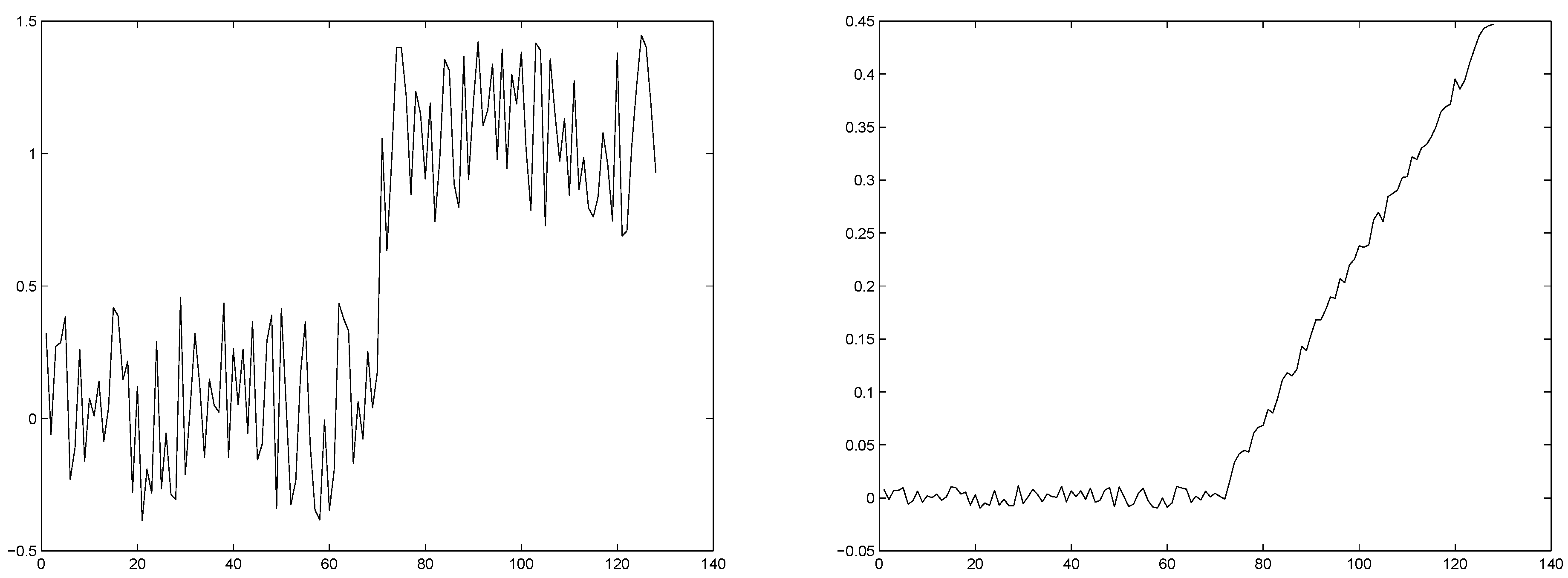
We consider both a jump and a corner. In Figure 1, we plot the signals and in Figure 2, their perturbations adding random noise. We use 64 points, and the noise size is less than and , respectively. These sizes are the biggest that we can consider, since a greater noise size value implies that the algorithm does not detect the discontinuities. We observe that the noise size to detect jumps is bigger than that considered in the literature that we have included. Moreover, we are able to find discontinuities in the derivatives (corners).
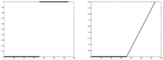
Figure 1.
(Left) jump, (right) corner.
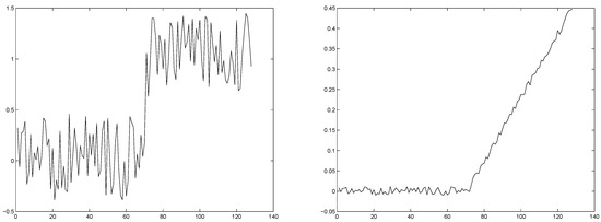
Figure 2.
(Left) jump with noise, (right) corner with noise.
In Table 4, we can observe good resolution of the detector. The algorithm can detect the true singularities even with significant noise present.

Table 4.
, Cell-average framework.
5. Application to the Detection of Heart Rate According to the Different Phases during Physical Exercise: Rest, Activation, Effort And Recovery
In this section, we apply our algorithm to the signals provided by heart rate monitoring devices placed on athletes. We discuss first the importance of monitoring the heart rate, how these signals are obtained and how the information extracted by applying our algorithm to them can be useful for the coaching staff of handball teams.
Within the realm of sports and the monitoring of physical activity, tracking heart rate has emerged as a vital tool for both athletes and fitness enthusiasts. This fundamental metric offers valuable insights into an individual’s physiological response to exercise, providing a glimpse into the body’s performance and overall well-being. Heart rate, measured in beats per minute (bpm), serves as an indicator of how effectively the cardiovascular system is operating and adapting during physical exertion. In the high-speed and physically challenging domain of handball, the monitoring of heart rate assumes a pivotal role in evaluating and enhancing performance.
To measure heart rate, dedicated devices like heart rate monitors, smartwatches, and chest straps are commonly used. Chest straps, specifically, are often equipped with electrodes that detect the electrical activity of the heart. They operate based on electrocardiography (ECG or EKG) principles, providing accurate and real-time heart rate data. This technology is widely used in fitness monitoring, sports training and medical applications. Our data were obtained using chest straps.
Advancements in wearable technology have enabled healthcare professionals and researchers to conveniently evaluate diverse health and fitness parameters. Portable devices, specifically designed for convenient heart rate variability recordings, have been developed, see [12]. Measurements of heart rate variability obtained through portable devices show a minimal level of absolute error, as indicated by [13]. Despite this slight variance, it is considered acceptable, given the improved practicality and compliance of heart rate variability measurements in real-world settings, see the review paper [14] for more details.
Next, we introduce a couple of examples that demonstrate the use of this algorithm during a match. The information obtained can be used by the coach for player rotations. Additionally, heart rate is an important indicator acting as an alert for potential cardiac anomalies.
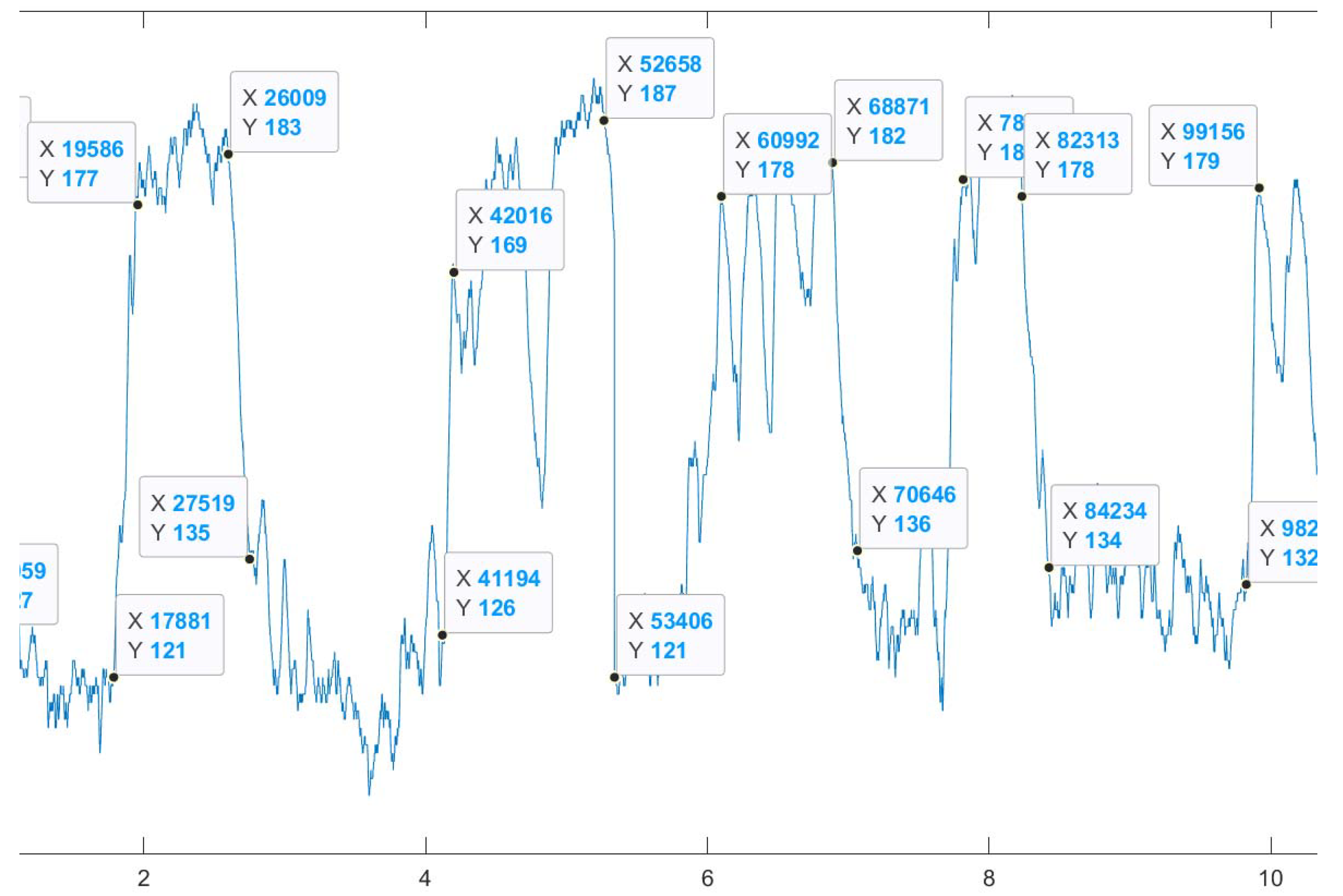
In Figure 3, we observe the detection of the different phases of exercise during a match. Moreover, with this detection, we can estimate the slopes between the different zones. The size of the slope is related to the physical form of the player. We can examine previously captured data to determine the physical evolution.
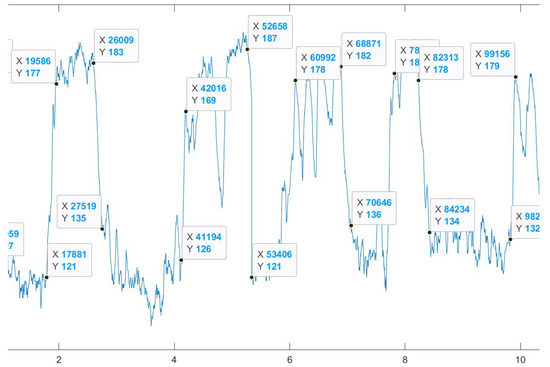
Figure 3.
Heart rate during a handball game. Detection of the different zones.
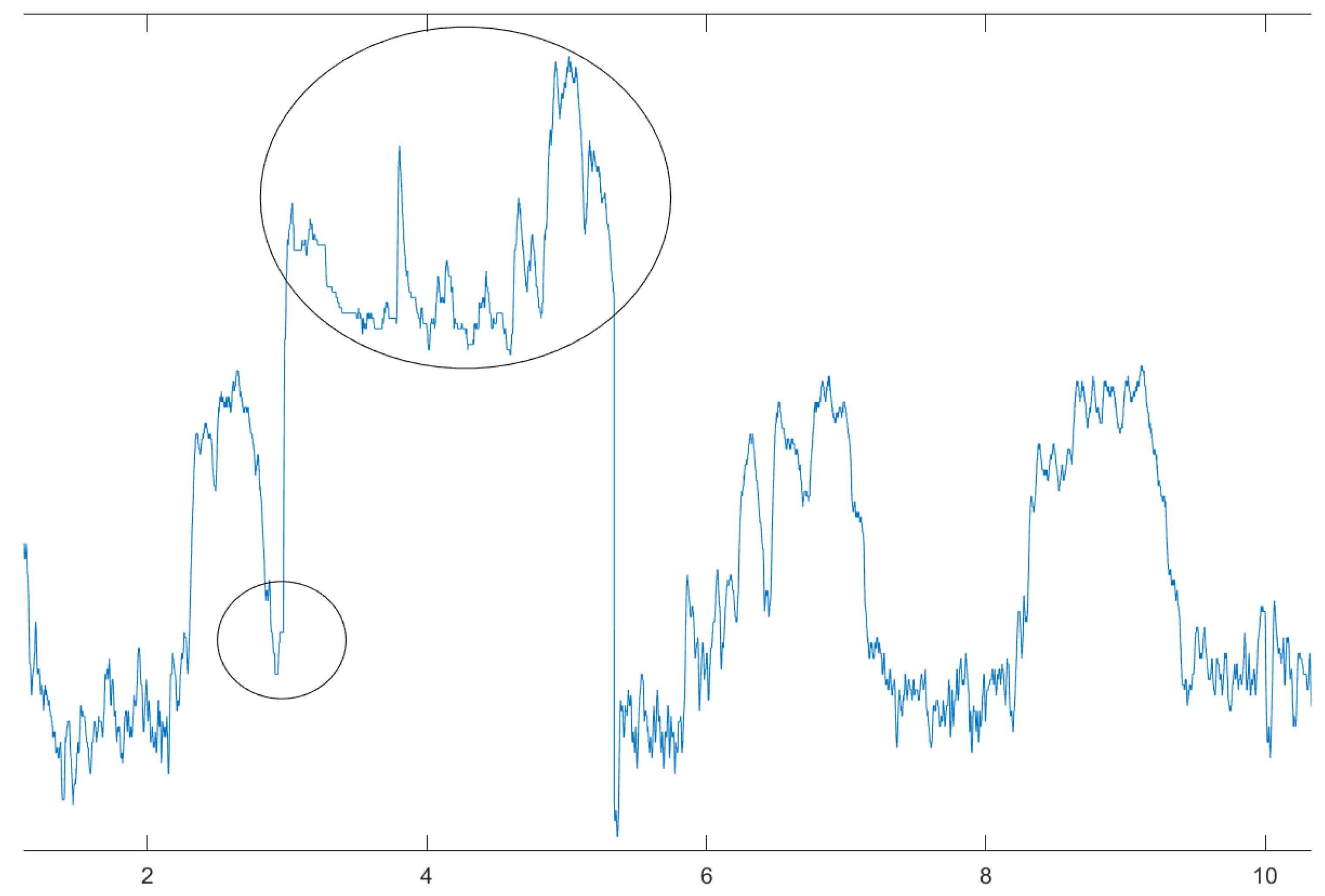
In Figure 4, we observe a heart rate that is excessively high due to a lack of rest. The coach called a timeout to provide rest, but the heart rate did not decrease sufficiently. Upon resuming the exercise, the heart rate spiked. This led to the detection of a minor cardiac anomaly in the athlete.
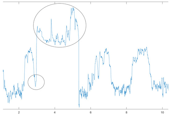
Figure 4.
Heart rate during a handball game. Detection of a cardiac anomaly.
6. Conclusions
In this work, we introduced a discontinuity detector for signals with noise. Both corners and jumps can be detected, and their sizes measured. The algorithm is an adaptation of Harten’s ENO-subcell resolution approach to the presence of noise. After testing the algorithm, it was applied to the detection of different phases of exercise during a handball match. This monitoring can assist in player rotations by indicating when a player has reached their recovery zone. Additionally, over time, the measurement of slopes separating different zones provides information on the evolution of the athlete’s physical condition. Finally, it is worth emphasizing that monitoring heart rate during exercise can help detect cardiac anomalies.
Another application we are interested in investigating involves combining our detector with some new approximations of piecewise functions in several dimensions that we have developed in recent works [15,16,17,18].
Author Contributions
Conceptualization, S.A. and S.B.; methodology, S.A.; software, S.B. and D.O.; validation, S.A., S.B. and D.O.; formal analysis, S.A. and S.B.; investigation, S.A., S.B. and D.O.; resources, S.A., S.B. and D.O.; writing—original draft preparation, S.A., S.B. and D.O.; writing—review and editing, S.A., S.B. and D.O. All authors have read and agreed to the published version of the manuscript.
Funding
This research received no external funding.
Data Availability Statement
Data are contained within the article.
Conflicts of Interest
The authors declare no conflict of interest.
References
- Harten, A. Discrete Multiresolution Analysis and Generalized Wavelets. J. Appl. Numer. Math. 1993, 12, 153–192. [Google Scholar]
- Harten, A. Multiresolution Representation of Data II: General Framework. SIAM J. Numer. Anal. 1996, 33, 1205–1256. [Google Scholar] [CrossRef]
- Kutyniok, G.; Petersen, P. Classification of edges using compactly supported shearlets. Appl. Comput. Harmon. Anal. 2017, 42, 245–293. [Google Scholar] [CrossRef]
- Guo, K.; Labate, D. Characterization and analysis of edges in piecewise smooth functions. Appl. Comput. Harmon. Anal. 2016, 41, 139–163. [Google Scholar] [CrossRef]
- Zhong, J.; Ning, R. Image Denoising Based on Wavelets and Multifractals for Singularity Detection. IEEE Trans. Image Process. 2005, 14, 1435. [Google Scholar] [CrossRef]
- Rakowki, W. Application of Cubic Box Spline Wavelets in the Analysis of Signal Singularities. Int. J. Appl. Math. Comput. Sci. 2015, 25, 927–941. [Google Scholar] [CrossRef]
- Canny, J. A computational approach to edge detection. IEEE Trans. Pattern Anal. Mach. Intell. 1986, 8, 679–714. [Google Scholar] [CrossRef] [PubMed]
- Dim, J.R.; Takamura, T. Alternative Approach for Satellite Cloud Classification: Edge Gradient Application. Adv. Meteorol. 2013, 2013, 584816. [Google Scholar] [CrossRef]
- Ziou, D.; Tabbone, S. Edge detection techniques: An overview. Int. J. Pattern Recognit. Image Anal. 1998, 8, 537–559. [Google Scholar]
- Yager, N.; Amin, A. Fingerprint classification: A review. Pattern Anal. Appl. 2004, 7, 77–93. [Google Scholar] [CrossRef]
- Aràndiga, F.; Cohen, A.; Donat, R.; Dyn, N. Interpolation and Approximation of Piecewise Smooth Functions. SIAM J. Numer. Anal. 2005, 43, 41–57. [Google Scholar] [CrossRef]
- Dobbs, W.C.; Fedewa, M.V.; MacDonald, H.V.; Holmes, C.J.; Cicone, Z.S.; Plews, D.J.; Esco, M.R. The accuracy of acquiring heart rate variability from portable devices: A systematic review and meta-analysis. Sport. Med. 2019, 49, 417–435. [Google Scholar] [CrossRef] [PubMed]
- Fuller, D.; Colwell, E.; Low, J.; Orychock, K.; Tobin, M.A.; Simango, B.; Taylor, N.G. Reliability and validity of commercially available wearable devices for measuring steps, energy expenditure, and heart rate: Systematic review. JMIR mHealth uHealth 2020, 8, e18694. [Google Scholar] [CrossRef] [PubMed]
- Georgiou, K.; Larentzakis, A.V.; Khamis, N.N.; Alsuhaibani, G.I.; Alaska, Y.A.; Giallafos, E.J. Can Wearable Devices Accurately Measure Heart Rate Variability? A Systematic Review. Folia Med. I 2018, 60, 7–20. [Google Scholar] [CrossRef] [PubMed]
- Amat, S.; Levin, D.; Ruiz-Álvarez, J. A two-stage approximation strategy for piecewise smooth functions in two and three dimensions. IMA J. Numer. Anal. 2022, 42, 3330–3359. [Google Scholar] [CrossRef]
- Amat, S.; Levin, D.; Ruiz-Álvarez, J.; Yáñez, D. Global and explicit approximation of piecewise-smooth two-dimensional functions from cell-average data. IMA J. Numer. Anal. 2023, 43, 2299–2319. [Google Scholar] [CrossRef]
- Amat, S.; Levin, D.; Ruiz-Álvarez, J.; Trillo, J.C.; Yáñez, D. A class of C2 quasi-interpolating splines free of Gibbs phenomenon. Numer. Algorithms 2022, 91, 51–79. [Google Scholar] [CrossRef]
- Amat, S.; Li, Z.; Ruiz-Álvarez, J. On an New Algorithm for Function Approximation with Full Accuracy in the Presence of Discontinuities Based on the Immersed Interface Method. J. Sci. Comput. 2018, 75, 1500–1534. [Google Scholar] [CrossRef]
Disclaimer/Publisher’s Note: The statements, opinions and data contained in all publications are solely those of the individual author(s) and contributor(s) and not of MDPI and/or the editor(s). MDPI and/or the editor(s) disclaim responsibility for any injury to people or property resulting from any ideas, methods, instructions or products referred to in the content. |
© 2024 by the authors. Licensee MDPI, Basel, Switzerland. This article is an open access article distributed under the terms and conditions of the Creative Commons Attribution (CC BY) license (https://creativecommons.org/licenses/by/4.0/).


