A Note on the Time-Fractional Navier–Stokes Equation and the Double Sumudu-Generalized Laplace Transform Decomposition Method

Abstract

In this work, the time-fractional Navier–Stokes equation is discussed using a calculational method, which is called the Sumudu-generalized Laplace transform decomposition method (DGLTDM). The fractional derivatives are defined in the Caputo sense. The (DGLTDM) is a hybrid of the Sumudu-generalized Laplace transform and the decomposition method. Three examples of the time-fractional Navier–Stokes equation are studied to check the validity and demonstrate the effectiveness of the current method. The results show that the suggested method succeeds remarkably well in terms of proficiency and can be utilized to study more problems in the field of nonlinear fractional differential equations (FDEs).

1. Introduction

Fractional partial differential equations play an important role in applied mathematics, as they have been suggested for and applied in several different areas of the physical sciences and engineering such as in fluid dynamics, acoustics, electromagnetism, visco-elasticity, electro-chemistry, etc. The authors in [1] discussed the multi-scale elastic structures consisting of matrix medium and thin coatings or inclusions. There are some approaches to solving the problem of the elastic deformation of thin-walled solids with a complex shape that is analyzed based on linear and geometrically nonlinear models using new classes of surfaces [2]. The researchers in [3] applied the variational method to solve the time-fractal heat conduction problem in the playdate–block construction.

The Navier–Stokes equations are commonly utilized to explain the motion of fluids in models related to weather, ocean currents, and water flow in a pipe. Also, Navier–Stokes equations are vector equations. Newly, several researchers have generalized the classical Navier–Stokes equation into a fractional formula depending on replacing the first-time derivative with a fractional derivative of order $0<\beta \le 1,$ as in [4,5,6,7,8].

Recently, several analytical and approximate techniques for solving time-fractional Navier–Stokes equations have been developed, for example, the Adomian decomposition method [9], the q-homotopy analysis transform scheme [10], the modified Laplace decomposition method [7], the Natural Homotopy Perturbation Method [11], a reliable algorithm based on the new homotopy perturbation transform method [6], and a modified reduced differential transform method [12]. In the paper [13], the authors discussed the convergence properties of double Sumudu transformation and applied it to obtain the exact solution of the Volterra integro-partial differential equation. The double Sumudu transform is connected with the Adomian decomposition method to obtain the analytical solution of nonlinear fractional partial differential equations [14].

The double Sumudu-generalized Laplace decomposition method is a strong method that has been used to develop the double Sumudu transform and generalized Laplace transform [15,16].

This work aims to study the time-fractional Navier–Stokes equation in one and two dimensions using the double Sumudu-generalized Laplace transform decomposition method and to determine the accuracy, efficiency, and simplicity of the suggested method.

lNotations:

In this paper, we employ the following symbols:

(1) (SGLT) instead of “Sumudu-generalized Laplace transform”;

(2) (DST) instead of “double Sumudu transform”;

(3) (DSGLT) instead of “double Sumudu-generalized Laplace transform”;

(4) (DM) instead of “decomposition method”;

(5) (DSGLTDM) instead of “double Sumudu-generalized Laplace transform decomposition method”.

This article is organized as follows. In Section 2, some definitions regarding fractional calculus and (SGLT) are given. In Section 3, the two main theorems are proved, which are useful to study the time-fractional Navier-Stokes equation constructed using the (SGLT). In Section 3.1, the (SGLTDM) is used to solve the one-dimensional time-fractional Navier–Stokes model. In Section 3.2, the (SGLTDM) is applied to solve the two-dimensional coupled time-fractional Navier–Stokes model. In Section 4 some numerical example are given. In Section 5, conclusions are given.

2. Basic Definitions of Fractional Derivatives and Sumudu-Generalized Laplace Transforms

In this part, some basic definitions of fractional calculus and (SGLT) are given, which are helpful for this paper.

Definition 1 

([10]). A real function $f\left(t\right)$, $t>0$ is is called in the space $C_{\mu }$, $\mu \in \mathbb{R}$ if $\exists p$ is a real number $p(>\mu )$, so that $f\left(t\right)=t^p{f}_1\left(t\right)$, where $f_1\left(t\right)\in C[0,\infty )$, and it is reportedly in the space $C_{\mu }^m$ if and only if $f^{\left(m\right)}$∈$C_{\mu }$, $m\in \mathbb{N}.$

Definition 2 

([17,18,19]). The Caputo time-fractional derivative operator of order $\tau >0$ is given by

$$D_t^{\tau }{u(x,t)=\{}_{\frac{{\partial }^{m}u(x,t)}{\partial t^m},\mathrm{for}m=\tau \in \mathbb{N}}^{\frac{1}{\mathrm{\Gamma }\left(m-\tau \right)}{\int }_0^t{\left(t-\sigma \right)}^{m-\tau -1}\frac{{\partial }^{m}u(x,\sigma )}{\partial {\sigma }^m}d\sigma ,}m-1<\tau <m.$$

(1)

Definition 3 

([20]). Let f be a function of two variables x and t, where $x,t>0$. The Sumudu-generalized Laplace transform of f is defined by

$$S_x{G}_t\left(f\left(x,t\right)\right)=F\left(u_1,s\right)=\frac{s^{\alpha }}{u_1}{\int }_0^{\infty }{\int }_0^{\infty }{e}^{-\left(\frac{x}{u_1}+\frac{t}{s}\right)}f\left(x,t\right)dtdx,$$

(2)

where the symbol $S_x{G}_t$ denoted the (SGLT), and the symbols $u_1$ and s denoted transforms of the variables x and t in (SGLT), respectively. Double Sumudu-generalized Laplace transform, which is defined by

$$S_x{S}_y{G}_t\left(f\left(x,y,t\right)\right)=\frac{s^{\alpha }}{u_1{u}_2}{\int }_0^{\infty }{\int }_0^{\infty }{\int }_0^{\infty }{e}^{-\left(\frac{x}{u_1}+\frac{y}{u_2}+\frac{t}{s}\right)}f\left(x,y,t\right)dtdydx.$$

(3)

Similarly, the (SGLT) for the second partial derivative with respect to x and t is defined as follows

$$L_x{G}_t\left[{\psi }_{xx}\right]=\frac{{\mathrm{\Psi }}_{\alpha }\left(u_1,s\right)}{u_1^2}-\frac{{\mathrm{\Psi }}_{\alpha }\left(0,s\right)}{u_1^2}-\frac{\partial {\mathrm{\Psi }}_{\alpha }\left(0,s\right)}{\partial x}.$$

$$\begin{array}{ccc}\hfill S_x{G}_t\left[{\psi }_t\right]& =& \frac{{\mathrm{\Psi }}_{\alpha }\left(u_1,s\right)}{s}-s^{\alpha }\mathrm{\Psi }\left(u_1,0\right),\hfill \\ \hfill S_x{G}_t\left[{\psi }_{tt}\right]& =& \frac{{\mathrm{\Psi }}_{\alpha }(u_1,s)}{s^2}-s^{\alpha -1}\mathrm{\Psi }(u_1,0)-s^{\alpha }{\mathrm{\Psi }}_t(u_1,0).\hfill \end{array}$$

In general,

$$\begin{array}{ccc}\hfill S_x{G}_{\alpha }\left[\frac{{\partial }^{m}f(x,t)}{\partial t^m}\right]& =& \frac{F_{\alpha }\left(u_1,s\right)}{s^m}\hfill \\ & & -s^{\alpha }\sum _{k=1}^n\frac{1}{s^{m-k}}{S}_x\left[\frac{{\partial }^{k-1}f\left(x,0\right)}{\partial t^{k-1}}\right].\hfill \end{array}$$

(4)

where $u_1,s$ are complex values. The inverse (SGLT) $S_{u_1}^{-1}{G}_s^{-1}\left[S_x{G}_t\left(f\left(x,t\right)\right)\right]=f\left(x,t\right)$ is defined as in [20] by the complex double integral formula

$$f\left(x,t\right)=\frac{1}{{\left(2\pi i\right)}^2}{\int }_{\tau -i\infty }^{\tau -i\infty }{\int }_{y-i\infty }^{y-i}{e}^{\frac{1}{u_1}x+\frac{1}{s}t}{S}_x{G}_t\left[f\left(x,t\right)\right]dsd{u}_1.$$

3. Main Results

In the following theorem, we present the (SGLT) of the partial fractional Caputo derivatives

Theorem 1. 

The (SGLT) of the fractional partial derivatives $D_t^{\beta }\psi$ is denoted by

$$S_x{G}_t\left[D_t^{\beta }\psi \right]=\frac{{\mathrm{\Psi }}_{\alpha }\left(u_1,s\right)}{s^{\beta }}-s^{\alpha }{\displaystyle \sum }_{k=1}^{\infty }\frac{1}{s^{\beta -k}}{S}_x\left[\frac{{\partial }^{k-1}}{\partial t^{k-1}}\psi \left(x,0\right)\right]$$

Proof. 

By utilizing the definition of (SGLT), we have

$$S_x{G}_t\left[D_t^{\beta }\psi \right]=\frac{s^{\alpha }}{u_1}{\int }_0^{\infty }{\int }_0^{\infty }{e}^{-\left(\frac{x}{u_1}+\frac{t}{s}\right)}{D}_t^{\beta }\psi dtdx,$$

and with the help of Equation (1), we obtain

$$\begin{array}{ccc}& & S_x{G}_t\left[D_t^{\beta }\psi \right]\hfill \\ & =& \frac{s^{\alpha }}{u_1}{\int }_0^{\infty }{\int }_0^{\infty }{e}^{-\left(\frac{x}{u_1}+\frac{t}{s}\right)}\frac{1}{\mathrm{\Gamma }\left(m-\beta \right)}{\int }_0^t{\left(t-\zeta \right)}^{m-\beta -1}\frac{{\partial }^m\psi (x,\zeta )}{\partial {\zeta }^m}d\zeta dtdx\hfill \\ & =& \frac{1}{u_1}{\int }_0^{\infty }{e}^{-\frac{x}{u_1}}\left(\frac{1}{\mathrm{\Gamma }\left(m-\beta \right)}{s}^{\alpha }{\int }_0^{\infty }{\int }_{\zeta }^{\infty }\frac{e^{-\frac{t}{s}}}{{\left(t-\zeta \right)}^{\beta -m+1}}\frac{{\partial }^m\psi (x,\zeta )}{\partial {\zeta }^m}dtd\zeta \right)dx.\hfill \end{array}$$

Let $v=t-\zeta$.

$$\begin{array}{ccc}& & S_x{G}_t\left[D_t^{\beta }\psi \right]\hfill \\ & =& \frac{1}{u_1}{\int }_0^{\infty }{e}^{-\frac{x}{u_1}}\left(\frac{s^{\alpha }}{\mathrm{\Gamma }\left(m-\beta \right)}{\int }_0^{\infty }\frac{{\partial }^m\psi (x,\zeta )}{\partial {\zeta }^m}d\zeta {\int }_0^{\infty }{v}^{m-\beta -1}{e}^{-\frac{\left(v+\zeta \right)}{s}}dv\right)dx\hfill \\ & =& \frac{1}{u_1}{\int }_0^{\infty }{e}^{-\frac{x}{u_1}}\left(\frac{s^{\alpha }}{\mathrm{\Gamma }\left(m-\beta \right)}{\int }_0^{\infty }{e}^{-\frac{\zeta }{s}}\frac{{\partial }^m\psi (x,\zeta )}{\partial {\zeta }^m}d\zeta {\int }_0^{\infty }{v}^{m-\beta -1}{e}^{-\frac{v}{s}}dv\right)dx\hfill \\ & =& \frac{1}{u_1}{\int }_0^{\infty }{e}^{-\frac{x}{u_1}}\left(\frac{s^{\alpha }}{\mathrm{\Gamma }\left(m-\beta \right)}{\int }_0^{\infty }{e}^{-\frac{\zeta }{s}}\frac{{\partial }^m\psi (x,\zeta )}{\partial {\zeta }^m}d\zeta \frac{\mathrm{\Gamma }\left(m-\beta \right)}{s^{\beta -m}}\right)dx\hfill \\ & =& \frac{1}{u_1}{\int }_0^{\infty }{e}^{-\frac{x}{u_1}}\left(s^{\alpha }{\int }_0^{\infty }{e}^{-\frac{\zeta }{s}}\frac{{\partial }^m\psi (x,\zeta )}{\partial {\zeta }^m}d\zeta \right)\frac{1}{s^{\beta -m}}dx,\hfill \end{array}$$

where

$$\frac{\mathrm{\Gamma }\left(m-\beta \right)}{s^{\beta -m}}={\int }_0^{\infty }{v}^{m-\beta -1}{e}^{-\frac{v}{s}}dv.$$

$$\begin{array}{ccc}& & S_x{G}_t\left[D_t^{\beta }\psi \right]\hfill \\ & =& \frac{1}{u_1}{\int }_0^{\infty }{e}^{-\frac{x}{u_1}}\left(G_t\left[\frac{{\partial }^m\psi (x,\zeta )}{\partial {\zeta }^m}\right]\right)\frac{1}{s^{\beta -m}}dx;\hfill \end{array}$$

by implementing Equation (4), we can obtain

$$S_x{G}_t\left[D_t^{\beta }\psi \right]=\frac{1}{s^{\beta -m}}\left[\frac{{\mathrm{\Psi }}_{\alpha }\left(u_1,s\right)}{s^m}-s^{\alpha }\sum _{k=1}^n\frac{1}{s^{m-k}}{S}_x\left[\frac{{\partial }^{k-1}\psi \left(x,0\right)}{\partial t^{k-1}}\right]\right];$$

by rewriting the equation above, we obtain

$$S_x{G}_t\left[D_t^{\beta }\psi \right]=\frac{{\mathrm{\Psi }}_{\alpha }\left(u_1,s\right)}{s^{\beta }}-s^{\alpha }\sum _{k=1}^n\frac{1}{s^{\beta -k}}{S}_x\left[\frac{{\partial }^{k-1}\psi \left(x,0\right)}{\partial t^{k-1}}\right].$$

□

In the next theorem, we utilize the (SGLT) for fractional partial derivatives $x{D}_t^{\beta }\psi .$

Theorem 2. 

The (SGLT) of the fractional partial derivatives $x{D}_t^{\beta }\psi$ is achieved by

$$\begin{array}{ccc}\hfill S_x{G}_t\left[x{D}_t^{\beta }\psi \right]& =& \frac{u_1}{s^{\beta }}\frac{d}{d{u}_1}\left(u_1{\mathrm{\Psi }}_{\alpha }(u_1,s)\right)\hfill \\ & & -u_1{s}^{\alpha -\beta +1}\frac{d}{d{u}_1}\left(u_1\mathrm{\Psi }(u_1,0)\right).\hfill \end{array}$$

(5)

Proof. 

By utilizing the derivatives with respect to $u_1$ for Equation (2), one can obtain

$$\begin{array}{ccc}\hfill \frac{d}{d{u}_1}\left(S_x{G}_t\left[D_t^{\beta }\psi \right]\right)& =& \frac{d}{d{u}_1}{\int }_0^{\infty }{\int }_0^{\infty }\frac{s^{\alpha }}{u_1}{e}^{-\left(\frac{1}{u_1}x+\frac{1}{s}t\right)}{D}_t^{\beta }\psi dxdt,\hfill \\ & =& {\int }_0^{\infty }{s}^{\alpha }{e}^{-\frac{1}{s}t}\left({\int }_0^{\infty }\frac{d}{d{u}_1}\frac{1}{u_1}{e}^{-\frac{1}{u_1}x}{D}_t^{\beta }\psi dx\right)dt;\hfill \end{array}$$

(6)

the derivative between the brackets can be calculated as follows:

$$\begin{array}{ccc}\hfill {\int }_0^{\infty }\frac{d}{d{u}_1}\frac{1}{u_1}{e}^{-\frac{1}{u_1}x}{D}_t^{\beta }\psi dx& =& {\int }_0^{\infty }\left(\frac{1}{u_1^3}x-\frac{1}{u_1^2}\right)e^{-\frac{1}{u_1}x}{D}_t^{\beta }\psi dx\hfill \\ & =& {\int }_0^{\infty }\frac{1}{u_1^3}x{e}^{-\frac{1}{u_1}x}{D}_t^{\beta }\psi dx\hfill \\ & & -{\int }_0^{\infty }\frac{1}{u_1^2}{e}^{-\frac{1}{u_1}x}{D}_t^{\beta }\psi dx;\hfill \end{array}$$

(7)

by putting Equation (7) into Equation (6), we obtain

$$\begin{array}{ccc}\hfill \frac{d}{d{\mu }_1}\left(S_x{G}_t\left[D_t^{\beta }\psi \right]\right)& =& {\int }_0^{\infty }{s}^{\alpha }{e}^{-\frac{1}{s}t}{\int }_0^{\infty }\frac{1}{u_1^3}x{e}^{-\frac{1}{u_1}x}{D}_t^{\beta }\psi dxdt\hfill \\ & & -{\int }_0^{\infty }{s}^{\alpha }{e}^{-\frac{1}{s}t}{\int }_0^{\infty }\frac{1}{u_1^2}{e}^{-\frac{1}{u_1}x}{D}_t^{\beta }\psi dxdtl\hfill \end{array}$$

(8)

consequently Equation (8) becomes

$$\begin{array}{ccc}\hfill \frac{d}{d{\mu }_1}\left(S_x{G}_t\left[D_t^{\beta }\psi \right]\right)& =& \frac{1}{u_1^2}\left(\frac{s^{\alpha }}{u_1}{\int }_0^{\infty }{\int }_0^{\infty }{e}^{-\left(\frac{1}{u_1}x+\frac{1}{s}t\right)}x{D}_t^{\beta }\psi dxdt\right)\hfill \\ & & -\frac{1}{u_1}\left(\frac{s^{\alpha }}{u_1}{\int }_0^{\infty }{\int }_0^{\infty }{e}^{-\left(\frac{1}{u_1}x+\frac{1}{s}t\right)}{D}_t^{\beta }\psi dxdt\right).\hfill \end{array}$$

(9)

Hence,

$$\begin{array}{ccc}\hfill \frac{d}{d{\mu }_1}\left(S_x{G}_t\left[D_t^{\beta }\psi \right]\right)& =& \frac{1}{u_1^2}{S}_x{G}_t\left[x{D}_t^{\beta }\psi \right]-\frac{1}{u_1}{S}_x{G}_t\left[D_t^{\beta }\psi \right];\hfill \end{array}$$

(10)

by managing the above equation, we will obtain the proof of Equation (5) as follows

$$\begin{array}{ccc}\hfill S_x{G}_t\left[x{D}_t^{\beta }\psi \right]& =& \frac{u_1}{s^{\beta }}\frac{d}{d{u}_1}\left(u_1{\mathrm{\Psi }}_{\alpha }(u_1,s)\right)\hfill \\ & & -u_1{s}^{\alpha -\beta +1}\frac{d}{d{u}_1}\left(u_1{\mathrm{\Psi }}_{\alpha }(u_1,0)\right).\hfill \end{array}$$

The proof is complete. □

The double Sumudu-generalized Laplace transform of the partial derivatives $D_t^{\beta }\psi \left(x,y,t\right)$ is given by

$$S_x{G}_t\left[\frac{{\partial }^{\beta }\psi \left(x,y,t\right)}{\partial t^{\beta }}\right]=\frac{{\mathrm{\Psi }}_{\alpha }\left(u_1,u_2,s\right)}{s^{\beta }}-s^{\alpha -\beta +1}{S}_x{S}_y\left[\mathrm{\Psi }\left(x,y,0\right)\right],$$

(11)

where $\beta$ represents the order of the derivative.

3.1. Analysis of the Sumudu-Generalized Laplace Decomposition Method

This subsection gives the main concept of the (SGLTDM) for the fractional partial differential equation, to demonstrate the essential strategy of the Sumudu-generalized Laplace Adomian decomposition method. The Navier–Stokes equation with time-fractional is denoted by

$$\begin{array}{ccc}\hfill D_t^{\beta }\psi (x,t)& =& D_x^{2}u(x,t)+\frac{1}{x}{D}_{x}u(x,t)+f(x,t),x,t>0,\hfill \\ \hfill m-1& <& \alpha <m,\hfill \end{array}$$

(12)

with the initial condition

$$\psi (x,0)=f_1\left(x\right),$$

where $D_t^{\beta }=\frac{{\partial }^{\beta }}{\partial t^{\beta }}$ is the fractional Caputo derivative, $D_x^2=\frac{{\partial }^2}{\partial x^2},$$D_x=\frac{\partial }{\partial x}$, and the right-hand-side function $f(x,t)$ is the source term. With a view to applying the (SGLTDM), the following steps are needed.

Step 1: We multiply first Equation (12) by $x,$ and we obtain

$$x{D}_t^{\alpha }\psi =x{D}_x^2\psi +D_x\psi +xf(x,t),x,t>0.$$

(13)

Step 2: Applying the (SGLT) on both sides of Equation (13), we have

$$S_x{G}_t\left[x{D}_t^{\alpha }\psi \right]=S_x{G}_t\left[x{D}_x^2\psi +D_x\psi +xf(x,t)\right],x,t>0.$$

(14)

Using Theorem 2, we obtain

$$\begin{array}{ccc}& & \frac{u_1}{s^{\beta }}\frac{d}{d{u}_1}\left(u_1{\mathrm{\Psi }}_{\alpha }(u_1,s)\right)-u_1{s}^{\alpha -\beta +1}\frac{d}{d{u}_1}\left(u_1{\mathrm{\Psi }}_{\alpha }(u_1,0)\right)\hfill \\ & =& S_x{G}_t\left[x{D}_x^2\psi +D_x\psi +xf(x,t)\right];\hfill \end{array}$$

after an algebraic handling, we obtain

$$\begin{array}{ccc}& & \frac{d}{d{u}_1}\left(u_1{\mathrm{\Psi }}_{\alpha }(u_1,s)\right)=s^{\alpha +1}\frac{d}{d{u}_1}\left(u_1{F}_1(u_1,0)\right)\hfill \\ & & +\frac{s^{\beta }}{u_1}{S}_x{G}_t\left[x{D}_x^2\psi +D_x\psi +xf(x,t)\right].\hfill \end{array}$$

(15)

Step 3: By employing the integral for both sides of Equation (15) from 0 to $u_1$ with respect to $u_1$, one can obtain

$$\begin{array}{ccc}\hfill {\mathrm{\Psi }}_{\alpha }(u_1,s)& =& s^{\alpha +1}{F}_1(u_1,0)+\frac{1}{u_1}{\int }_0^{u_1}\left(\frac{s^{\beta }}{u_1}{S}_x{G}_t\left[xf(x,t)\right]\right)d{u}_1\hfill \\ & & +\frac{1}{u_1}{\int }_0^{u_1}\left(\frac{s^{\beta }}{u_1}{S}_x{G}_t\left[x{D}_x^2\psi +D_x\psi \right]\right)d{u}_1.\hfill \end{array}$$

(16)

Step 4: By utilizing the inverse (SGLT) for Equation (16), we obtain

$$\begin{array}{ccc}\hfill \psi \left(x,t\right)& =& f_1\left(x\right)+S_{u_1}^{-1}{G}_s^{-1}\left[\frac{1}{u_1}{\int }_0^{u_1}\left(\frac{s^{\beta }}{u_1}{S}_x{G}_t\left[x{D}_x^2\psi +D_x\psi \right]\right)d{u}_1\right]\hfill \\ & & +S_{u_1}^{-1}{G}_s^{-1}\left[\frac{1}{u_1}{\int }_0^{u_1}\left(\frac{s^{\beta }}{u_1}{S}_x{G}_t\left[xf(x,t)\right]\right)d{u}_1\right],\hfill \end{array}$$

(17)

where the symbol $S_{u_1}^{-1}{G}_s^{-1}$ indicates the inverse (SGLT). The method (SGLTD M) designates the solution as an infinite series, as

$$\psi \left(x,t\right)={\displaystyle \sum }_{m=0}^{\infty }{\psi }_m\left(x,t\right);$$

(18)

by placing Equation (18) into Equation (16), we obtain

$$\begin{array}{ccc}\hfill {\displaystyle \sum }_{m=0}^{\infty }{\psi }_m\left(x,t\right)& =& f_1\left(x\right)+S_{u_1}^{-1}{G}_s^{-1}\left[\frac{1}{u_1}{\int }_0^{u_1}\left(\frac{s^{\beta }}{u_1}{S}_x{G}_t\left[xf(x,t)\right]\right)d{u}_1\right]\hfill \\ & & +S_{u_1}^{-1}{G}_s^{-1}\left[\frac{1}{u_1}{\int }_0^{u_1}\left(\frac{s^{\beta }}{u_1}{S}_x{G}_t\left[{\displaystyle \sum }_{m=0}^{\infty }\left(x{D}_x^2{\psi }_m+D_x{\psi }_m\right)\right]\right)d{u}_1\right].\hfill \end{array}$$

(19)

By using (SGLTDM), we present the iteration relations as:

$${\psi }_0\left(x,t\right)=f_1\left(x\right)+S_{u_1}^{-1}{G}_s^{-1}\left[\frac{1}{u_1}{\int }_0^{u_1}\left(\frac{s^{\beta }}{u_1}{S}_x{G}_t\left[xf(x,t)\right]\right)d{u}_1\right],$$

(20)

and the remaining terms can be acquired from the next formula

$${\psi }_{m+1}\left(x,t\right)=S_{u_1}^{-1}{G}_s^{-1}\left[\frac{1}{u_1}{\int }_0^{u_1}\left(\frac{s^{\beta }}{u_1}{S}_x{G}_t\left[\left(x{D}_x^2{\psi }_m+D_x{\psi }_m\right)\right]\right)d{u}_1\right].m\ge 1$$

(21)

We consider that the inverse exists for all terms on the right-hand side of Equations (20) and (21), respectively, where $S_x{G}_t$ is the (SGLT) with respect to $x,$t, and the inverse (SGLT) is given by $S_{u_1}^{-1}{G}_s^{-1}$ with respect to $u_1,$s.

3.2. Analysis of the Double Sumudu-Generalized Laplace Transforms Decomposition Method

In this part of the paper, we present the fundamental concept of the (DSGLTDM) for the time-fractional partial differential equation. To show the elementary plan of (DSGLTDM), we consider in the following a general coupled system two-dimensional time-fractional Navier–Stokes equations.

$$\begin{array}{ccc}\hfill D_t^{\beta }\psi +\psi {\psi }_x+\phi {\psi }_y& =& {\rho }_0\left({\psi }_{xx}+{\psi }_{yy}\right)-\frac{1}{\rho }\frac{\partial p}{\partial x},x,y,t>0,\hfill \\ \hfill D_t^{\beta }\phi +\psi {\phi }_x+\phi {\phi }_y& =& {\rho }_0\left({\phi }_{xx}+{\phi }_{yy}\right)-\frac{1}{\rho }\frac{\partial p}{\partial y},x,y,t>0,\hfill \\ \hfill n-1& <& \beta <n,\hfill \end{array}$$

(22)

subject to the conditions

$$\psi (x,y,0)=f_1(x,y),\phi (x,y,0)=g_1(x,y),$$

(23)

where $D_t^{\alpha }=\frac{{\partial }^{\alpha }}{\partial t^{\alpha }}$ is the fractional Caputo derivative, p is pressure; in addition, if p is known, then $q_1=$$\frac{1}{\rho }\frac{\partial p}{\partial x}$, and $q_2=-\frac{1}{\rho }\frac{\partial p}{\partial y}.$ The approach requires applying the (DSGLT) for both sides of Equation (22), and we obtain

$$\begin{array}{ccc}\hfill \frac{\mathrm{\Psi }\left(u_1,u_2,s\right)}{s^{\beta }}-s^{\alpha -\beta +1}\mathrm{\Psi }\left(u_1,u_2,0\right)& =& -S_x{S}_y{G}_t\left(\psi {\psi }_x+\phi {\psi }_y\right)\hfill \\ & & +S_x{S}_y{G}_t\left({\rho }_0\left({\psi }_{xx}+{\psi }_{yy}\right)\right)-S_x{S}_y{G}_t\left(q_1\right),\hfill \\ \hfill \frac{\mathrm{\Phi }\left(u_1,u_2,s\right)}{s^{\beta }}-s^{\alpha -\beta +1}\mathrm{\Phi }\left(u_1,u_2,0\right)& =& -S_x{S}_y{G}_t\left(\psi {\phi }_x+\phi {\phi }_y\right)\hfill \\ & & +S_x{S}_y{G}_t\left({\rho }_0\left({\phi }_{xx}+{\phi }_{yy}\right)\right)+S_x{S}_y{G}_t\left(q_2\right).\hfill \end{array}$$

(24)

Now, using the differentiation property of the (DST), we have

$$\begin{array}{ccc}\hfill \mathrm{\Psi }\left(u_1,u_2,s\right)& =& s^{\alpha -\beta +1}{F}_1\left(u_1,u_2\right)-s^{\beta }{S}_x{S}_y{G}_t\left(\psi {\psi }_x+\phi {\psi }_y\right)\hfill \\ & & +s^{\beta }{S}_x{S}_y{G}_t\left({\rho }_0\left({\psi }_{xx}+{\psi }_{yy}\right)\right)-s^{\beta }{S}_x{S}_y{G}_t\left(q_1\right),\hfill \\ \hfill \mathrm{\Phi }\left(u_1,u_2,s\right)& =& s^{\alpha -\beta +1}{G}_1\left(u_1,u_2\right)-s^{\beta }{S}_x{S}_y{G}_t\left(\psi {\phi }_x+\phi {\phi }_y\right)\hfill \\ & & +s^{\beta }{S}_x{S}_y{G}_t\left({\rho }_0\left({\phi }_{xx}+{\phi }_{yy}\right)\right)+s^{\beta }{S}_x{S}_y{G}_t\left(q_2\right).\hfill \end{array}$$

(25)

By involving the inverse (DSGLT) for Equation (25), we obtain

$$\begin{array}{ccc}\hfill \psi (x,y,t)& =& S_{u_1}^{-1}{S}_{u_2}^{-1}{G}_s^{-1}\left(s^{\alpha -\beta +1}{F}_1\left(u_1,u_2\right)\right)-S_{u_1}^{-1}{S}_{u_2}^{-1}{G}_s^{-1}\left(s^{\beta }{S}_x{S}_y{G}_t\left(\psi {\psi }_x+\phi {\psi }_y\right)\right)\hfill \\ & & +S_{u_1}^{-1}{S}_{u_2}^{-1}{G}_s^{-1}\left(s^{\beta }{S}_x{S}_y{G}_t\left({\rho }_0\left({\psi }_{xx}+{\psi }_{yy}\right)\right)\right)-S_{u_1}^{-1}{S}_{u_2}^{-1}{G}_s^{-1}\left[s^{\beta }{S}_x{S}_y{G}_t\left(q_1\right)\right],\hfill \\ \hfill \phi (x,y,t)& =& S_{u_1}^{-1}{S}_{u_2}^{-1}{G}_s^{-1}\left(s^{\alpha -\beta +1}{G}_1\left(u_1,u_2\right)\right)-S_{u_1}^{-1}{S}_{u_2}^{-1}{G}_s^{-1}\left(s^{\beta }{S}_x{S}_y{G}_t\left(\psi {\phi }_x+\phi {\phi }_y\right)\right)\hfill \\ & & +S_{u_1}^{-1}{S}_{u_2}^{-1}{G}_s^{-1}\left(s^{\beta }{S}_x{S}_y{G}_t\left({\rho }_0\left({\phi }_{xx}+{\phi }_{yy}\right)\right)\right)+S_{u_1}^{-1}{S}_{u_2}^{-1}{G}_s^{-1}\left[s^{\beta }{S}_x{S}_y{G}_t\left(q_2\right)\right].\hfill \end{array}$$

(26)

The DM presumes that the functional solutions to $\psi (x,y,t)$ and $\phi (x,y,t)$ are given by the following infinite series

$$\psi (x,y,t)={\displaystyle \sum }_{n=0}^{\infty }{\psi }_n(x,y,t),\phi (x,y,t)={\displaystyle \sum }_{n=0}^{\infty }{\phi }_n(x,y,t).$$

(27)

In addition, the nonlinear terms $\psi {\psi }_x,\phi {\psi }_y,\psi {\phi }_x$, and $\phi {\phi }_y$ are specified by

$$\psi {\psi }_x={\displaystyle \sum }_{n=0}^{\infty }{A}_n,\phi {\psi }_y={\displaystyle \sum }_{n=0}^{\infty }{B}_n,\psi {\phi }_x={\displaystyle \sum }_{n=0}^{\infty }{C}_n,\phi {\phi }_y={\displaystyle \sum }_{n=0}^{\infty }{D}_n.$$

(28)

By placing Equation (27) into Equation (25), we obtain

$$\begin{array}{ccc}\hfill {\displaystyle \sum }_{m=0}^{\infty }{\psi }_n(x,y,t)& =& f_1(x,y)-S_{u_1}^{-1}{S}_{u_2}^{-1}{G}_s^{-1}\left(s^{\beta }{S}_x{S}_y{G}_t\left({\displaystyle \sum }_{n=0}^{\infty }\left(A_n+B_n\right)\right)\right)\hfill \\ & & +S_{u_1}^{-1}{S}_{u_2}^{-1}{G}_s^{-1}\left(s^{\beta }{S}_x{S}_y{G}_t\left({\rho }_0\left({\displaystyle \sum }_{n=0}^{\infty }{\psi }_{nxx}+{\displaystyle \sum }_{n=0}^{\infty }{\psi }_{nyy}\right)\right)\right)\hfill \\ & & -S_{u_1}^{-1}{S}_{u_2}^{-1}{G}_s^{-1}\left[s^{\beta }{S}_x{S}_y{G}_t\left(q_1\right)\right],\hfill \end{array}$$

(29)

and

$$\begin{array}{ccc}\hfill {\displaystyle \sum }_{m=0}^{\infty }{\phi }_n(x,y,t)& =& g_1(x,y)-S_{u_1}^{-1}{S}_{u_2}^{-1}{G}_s^{-1}\left(s^{\beta }{S}_x{S}_y{G}_t\left({\displaystyle \sum }_{n=0}^{\infty }\left(C_n+D_n\right)\right)\right)\hfill \\ & & +S_{u_1}^{-1}{S}_{u_2}^{-1}{G}_s^{-1}\left(s^{\beta }{S}_x{S}_y{G}_t\left({\rho }_0\left({\displaystyle \sum }_{n=0}^{\infty }{\phi }_{nxx}+{\displaystyle \sum }_{n=0}^{\infty }{\phi }_{nyy}\right)\right)\right)\hfill \\ & & +S_{u_1}^{-1}{S}_{u_2}^{-1}{G}_s^{-1}\left[s^{\beta }{S}_x{S}_y{G}_t\left(q_2\right)\right].\hfill \end{array}$$

(30)

Using (DSGLTDM), we present the recursive relations as:

$$\begin{array}{ccc}\hfill u_0(x,y,t)& =& f_1\left(x,y\right)-S_{u_1}^{-1}{S}_{u_2}^{-1}{G}_s^{-1}\left[s^{\beta }{S}_x{S}_y{G}_t\left(q_1\right)\right]\hfill \\ \hfill v_0(x,y,t)& =& g_1\left(x,y\right)+S_{u_1}^{-1}{S}_{u_2}^{-1}{G}_s^{-1}\left[s^{\beta }{S}_x{S}_y{G}_t\left(q_2\right)\right],\hfill \end{array}$$

(31)

and the remaining elements ${\psi }_{n+1}$ and ${\phi }_{n+1},n\ge 0$ are denoted by

$$\begin{array}{ccc}\hfill {\psi }_{n+1}(x,y,t)& =& -S_{u_1}^{-1}{S}_{u_2}^{-1}{G}_s^{-1}\left(s^{\beta }{S}_x{S}_y{G}_t\left(A_n+B_n\right)\right)\hfill \\ & & +S_{u_1}^{-1}{S}_{u_2}^{-1}{G}_s^{-1}\left(s^{\beta }{S}_x{S}_y{G}_t\left({\rho }_0\left({\psi }_{nxx}+{\psi }_{nyy}\right)\right)\right),\hfill \end{array}$$

(32)

and

$$\begin{array}{ccc}\hfill {\phi }_{n+1}(x,y,t)& =& -S_{u_1}^{-1}{S}_{u_2}^{-1}{G}_s^{-1}\left(s^{\beta }{S}_x{S}_y{G}_t\left(C_n+D_n\right)\right)\hfill \\ & & +S_{u_1}^{-1}{S}_{u_2}^{-1}{G}_s^{-1}\left(s^{\beta }{S}_x{S}_y{G}_t\left({\rho }_0\left({\phi }_{nxx}+{\phi }_{nyy}\right)\right)\right).\hfill \end{array}$$

(33)

The inverse (DSGLT) is denoted by $S_{u_1}^{-1}{S}_{u_2}^{-1}{G}_s^{-1}$ with respect to $u_1,u_2,$s. We presume that the inverse (DSGLT), with respect to $u_1,u_2$ and s exist for Equations (31)–(33).

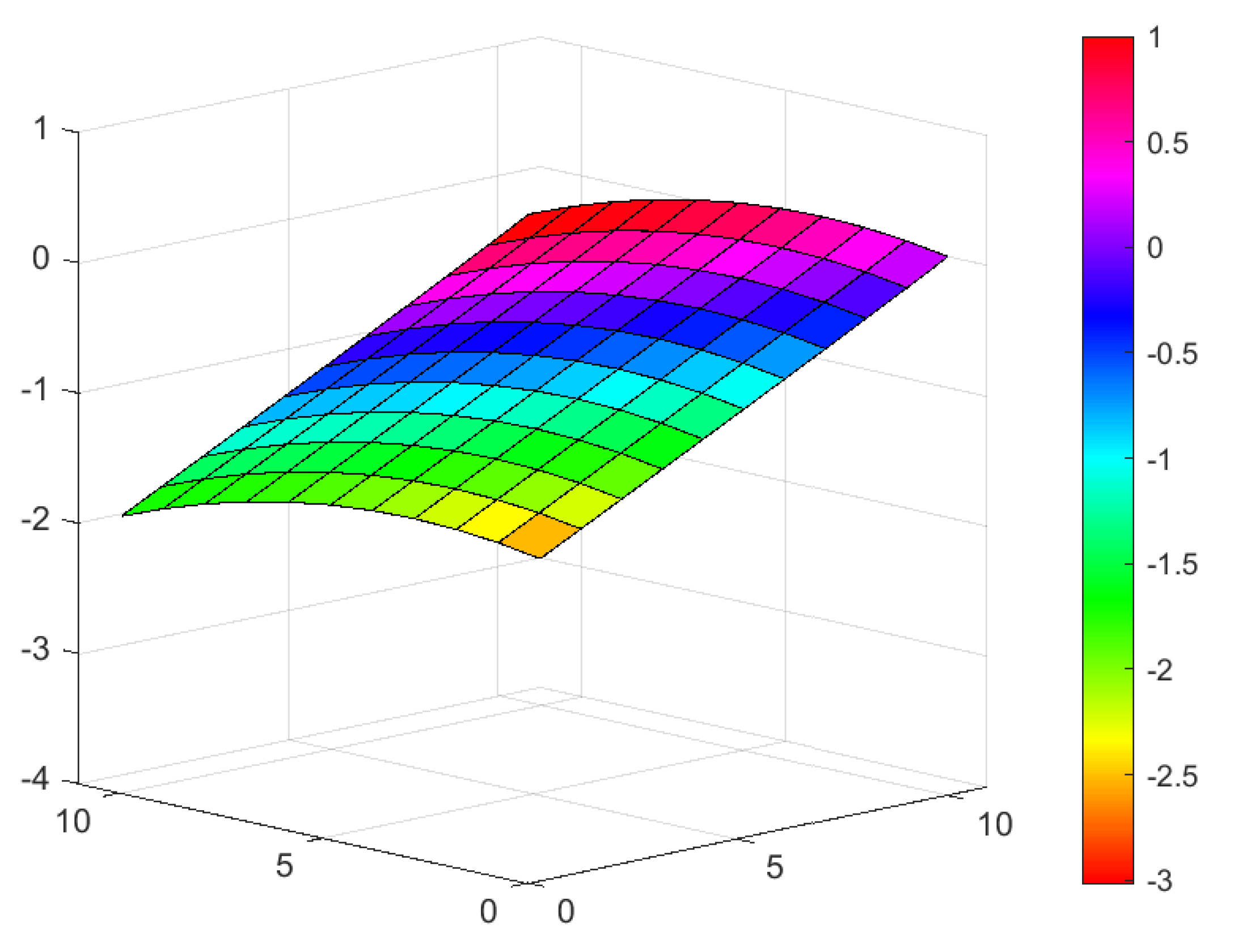
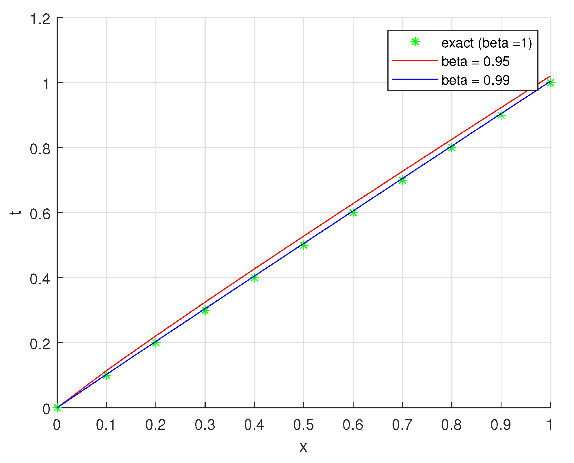
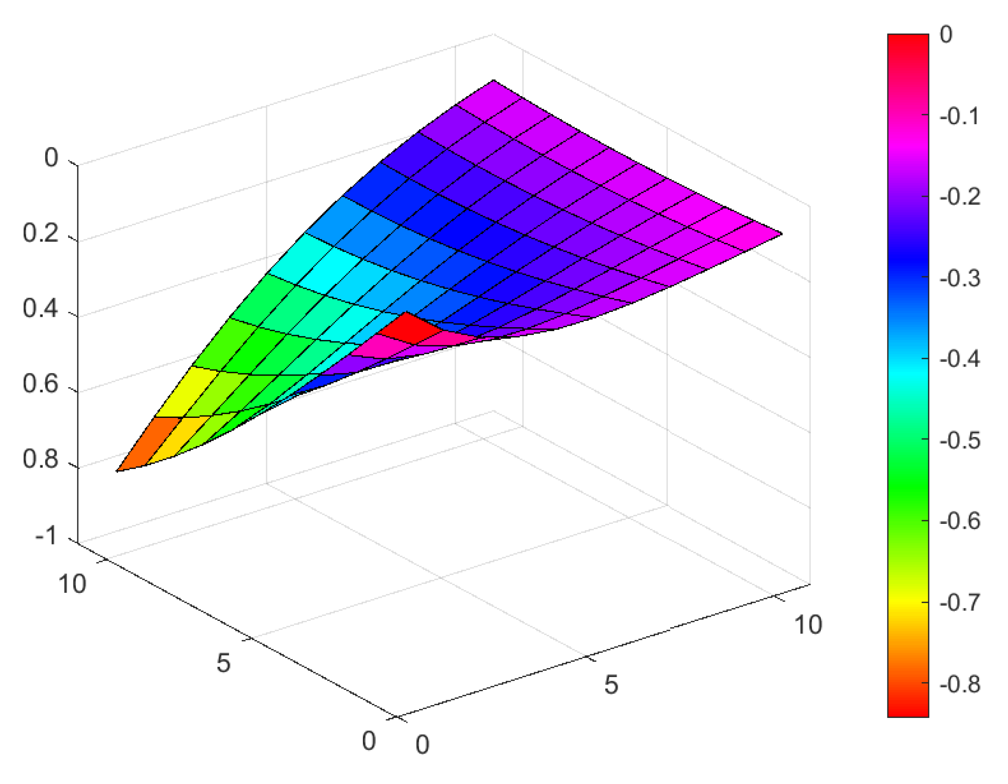
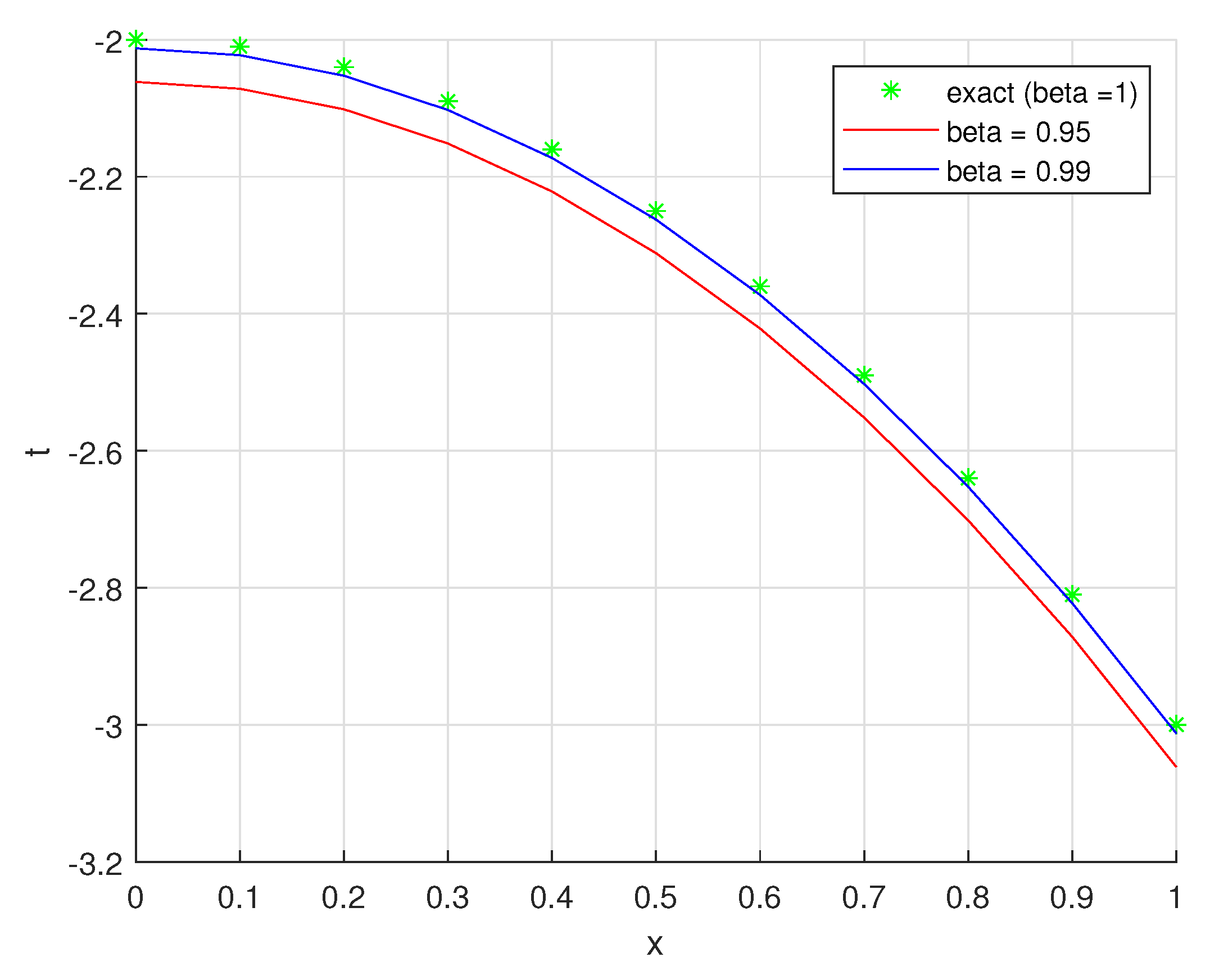
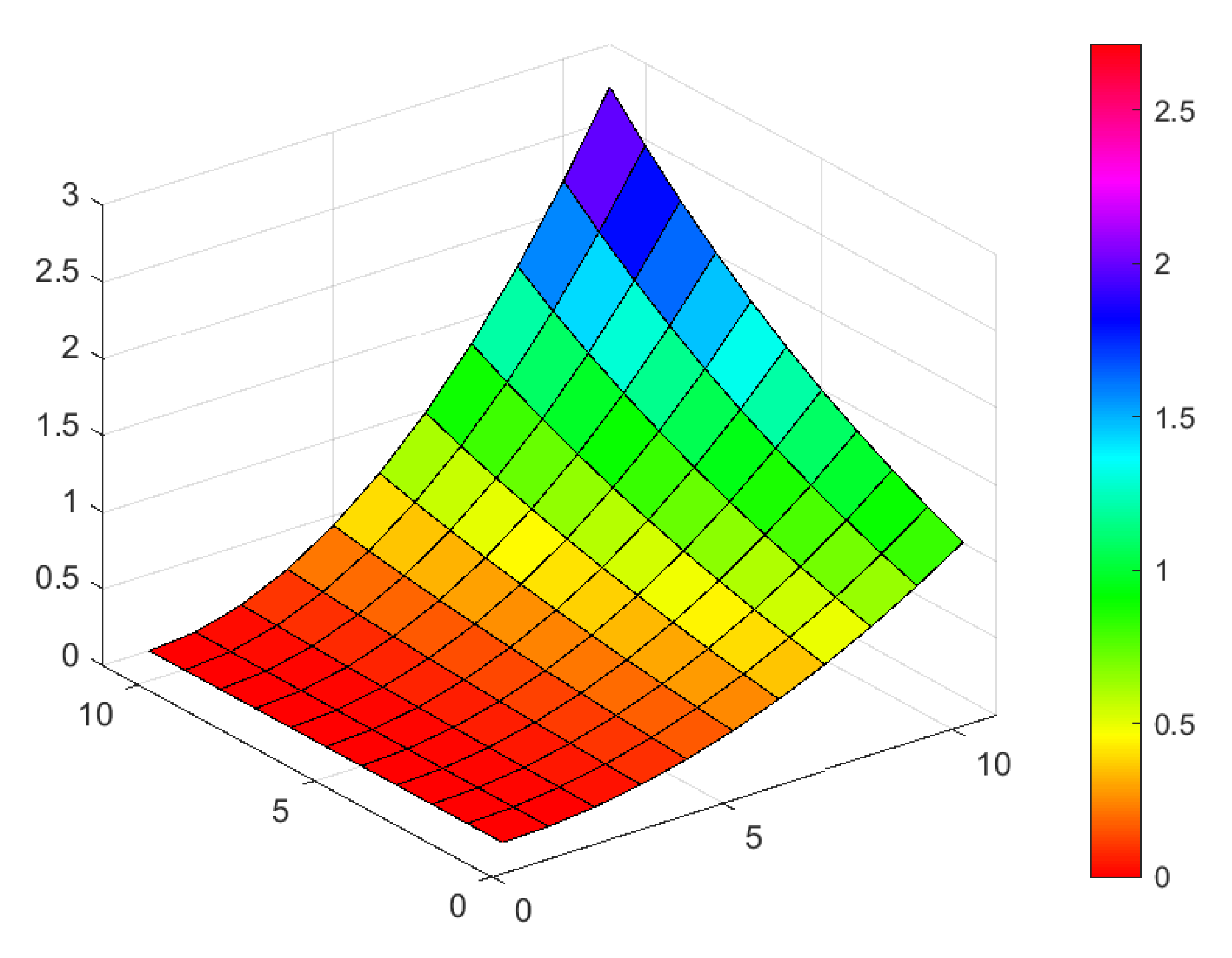
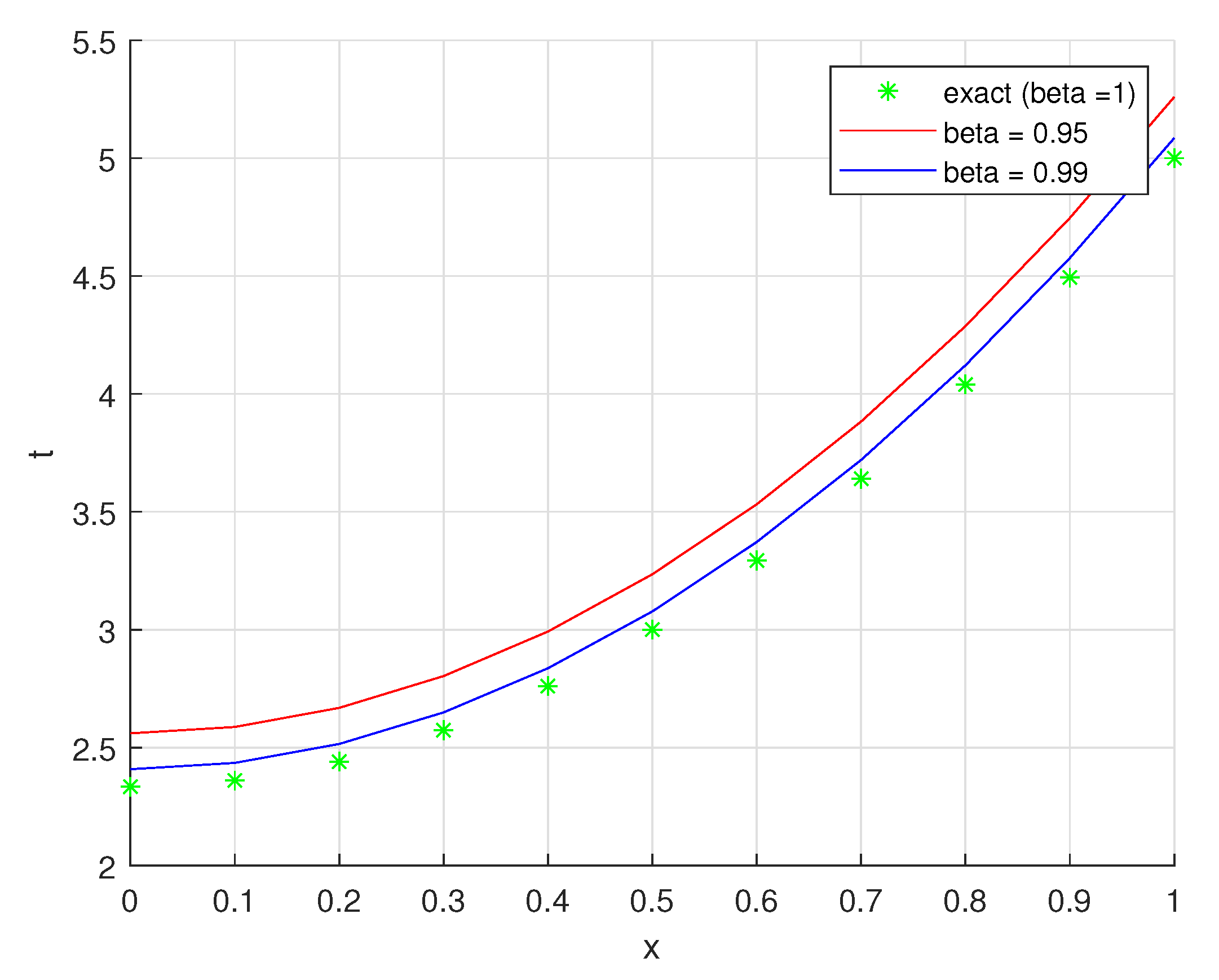
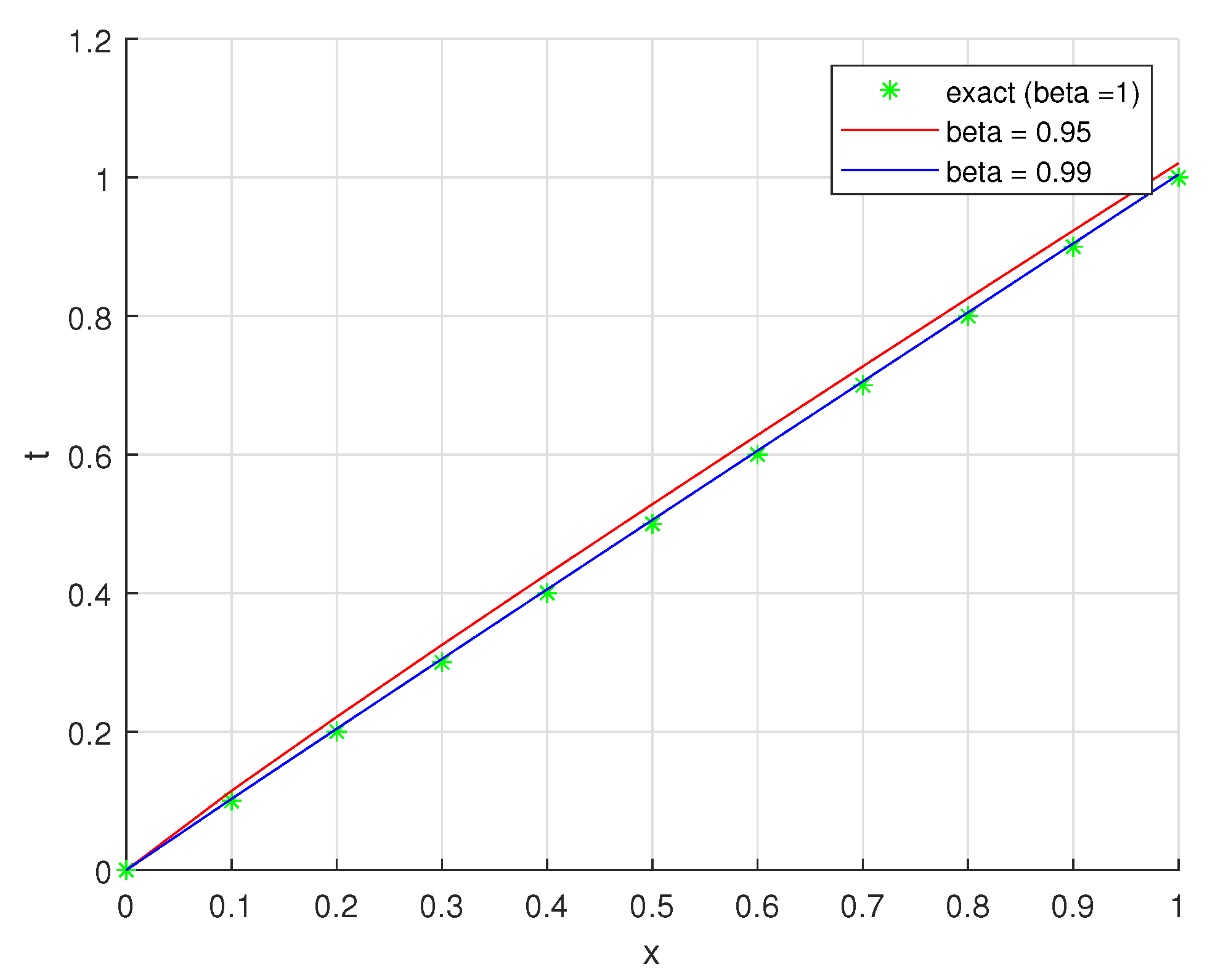
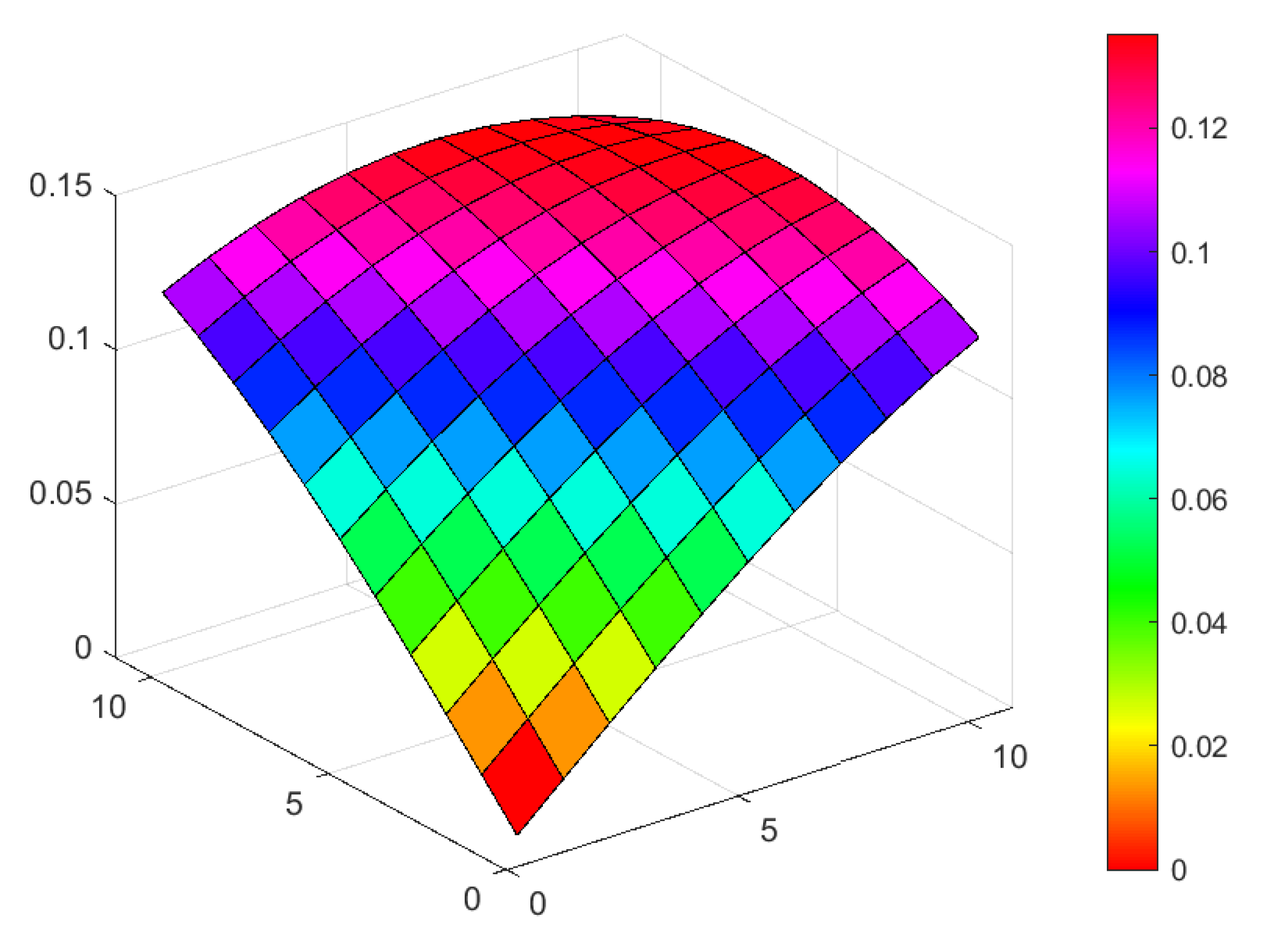
4. Numerical Examples

In this section, two problems on fractional homogeneous and non-homogeneous time-fractional Navier–Stokes equations are solved to verify the ability and dependability of our method (SGLTDM) and (DSGLTDM).

Example 1. 

Consider the following homogeneous one-dimensional motion of a dense fluid in a tube with the condition provided by

$$D_t^{\beta }\psi =-\frac{\partial p}{\rho \partial z}+\frac{v}{x}\frac{\partial }{\partial x}\left(x{D}_x\psi \right),x,t>0$$

(34)

and the initial condition

$$\psi \left(x,0\right)=1-x^2.$$

(35)

The fractional derivative model is used to illustrate the time derivative term, and Equation (34) can be written in the following form

$$D_t^{\beta }\psi =K+\frac{v}{x}\frac{\partial }{\partial x}\left(x{D}_x\psi \right),x,t>0,$$

(36)

where $K=$$-\frac{\partial p}{\rho \partial z};$ multiplying the above equation by x, we have

$$x{D}_t^{\beta }\psi =Kx+v\frac{\partial }{\partial x}\left(x{D}_x\psi \right),x,t>0.$$

(37)

By taking the (SGLT) for both sides of Equation (37), we arrive at

$$S_x{G}_t\left[x{D}_t^{\alpha }\psi \right]=S_x{G}_t\left[Kx\right]+S_x{G}_t\left[v\frac{\partial }{\partial x}\left(x{D}_x\psi \right)\right];$$

(38)

on using the differentiation property of the Sumudu transform and Theorem 2, we can obtain

$$\begin{array}{ccc}& & \frac{d}{d{u}_1}\left(u_1{\mathrm{\Psi }}_{\alpha }(u_1,s)\right)=s^{\alpha +1}\frac{d}{d{u}_1}\left(u_1{F}_1(u_1,0)\right)\hfill \\ & & +K{s}^{\alpha +1+\beta }+\frac{s^{\beta }}{u_1}{S}_x{G}_t\left[v\frac{\partial }{\partial x}\left(x{D}_x\psi \right)\right].\hfill \end{array}$$

(39)

Utilizing the Sumudu transform for the initial condition and substituting it into Equation (39), we have

$$\begin{array}{ccc}\hfill \frac{d}{d{u}_1}\left(u_1{\mathrm{\Psi }}_{\alpha }(u_1,s)\right)& =& \left(1-6u_1^2\right)s^{\alpha +1}+K{s}^{\alpha +1+\beta }\hfill \\ & & +\frac{s^{\beta }}{u_1}{S}_x{G}_t\left[v\frac{\partial }{\partial x}\left(x{D}_x\psi \right)\right];\hfill \end{array}$$

(40)

by taking the integral for both sides of Equation (40) from 0 to $u_1$ with respect to $u_1$ and dividing the results by $u_1$, we obtain

$$\begin{array}{ccc}\hfill {\mathrm{\Psi }}_{\alpha }(u_1,s)& =& \left(1-2u_1^2\right)s^{\alpha +1}+K{s}^{\alpha +1+\beta }\hfill \\ & & +\frac{1}{u_1}{\int }_0^{u_1}\frac{s^{\beta }}{u_1}{S}_x{G}_t\left[v\frac{\partial }{\partial x}\left(x{D}_x\psi \right)\right]d{u}_1.\hfill \end{array}$$

(41)

Now, the inverse (SGLT) of Equation (41) is given by

$$\begin{array}{ccc}\hfill \psi \left(x,t\right)& =& 1-x^2+\frac{K{t}^{\beta }}{\mathrm{\Gamma }\left(\beta +1\right)}\hfill \\ & & +S_{u_1}^{-1}{G}_s^{-1}\left[\frac{1}{u_1}{\int }_0^{u_1}\frac{s^{\beta }}{u_1}{S}_x{G}_t\left[v\frac{\partial }{\partial x}\left(x{D}_x\psi \right)\right]d{u}_1\right],\hfill \end{array}$$

(42)

and we assume an infinite series solution of the unknown function $\psi \left(x,t\right)$ is denoted by Equation (18). By substituting Equation (18) into Equation (42), we obtain:

$$\begin{array}{ccc}\hfill {\displaystyle \sum }_{m=0}^{\infty }{\psi }_m\left(x,t\right)& =& 1-x^2+\frac{K{t}^{\beta }}{\mathrm{\Gamma }\left(\beta +1\right)}\hfill \\ & & +S_{u_1}^{-1}{G}_s^{-1}\left[\frac{1}{u_1}{\int }_0^{u_1}\left(\frac{s^{\beta }}{u_1}{S}_x{G}_t\left[{\displaystyle \sum }_{m=0}^{\infty }v\frac{\partial }{\partial x}\left(x{D}_x{\psi }_m\right)\right]\right)d{u}_1\right].\hfill \end{array}$$

(43)

The zeroth component ${\psi }_0$ is recommended by the Adomian method, which always includes the initial condition and the source term, both of which are considered to be known. Therefore, we place

$${\psi }_0=1-x^2+\frac{K{t}^{\beta }}{\mathrm{\Gamma }\left(\beta +1\right)}.$$

The remaining components ${\psi }_{m+1}$, $m\ge 0$ are given by using the relation

$${\psi }_{m+1}\left(x,t\right)=S_{u_1}^{-1}{G}_s^{-1}\left[\frac{1}{u_1}{\int }_0^{u_1}\left(\frac{s^{\beta }}{u_1}{S}_x{G}_t\left[v\frac{\partial }{\partial x}\left(x{D}_x{\psi }_m\right)\right]\right)d{u}_1\right];$$

(44)

by substituting $m=0$, into Equation (44), we obtain

$$\begin{array}{ccc}\hfill {\psi }_1\left(x,t\right)& =& S_{u_1}^{-1}{G}_s^{-1}\left[\frac{1}{u_1}{\int }_0^{u_1}\left(\frac{s^{\beta }}{u_1}{S}_x{G}_t\left[v\frac{\partial }{\partial x}\left(x{D}_x{\psi }_0\right)\right]\right)d{u}_1\right]\hfill \\ & =& -S_{u_1}^{-1}{G}_s^{-1}\left[\frac{1}{u_1}{\int }_0^{u_1}\left[4v{s}^{\alpha +\beta +1}\right]dp\right]=-S_{u_1}^{-1}{G}_s^{-1}\left[4v{s}^{\alpha +\beta +1}\right].\hfill \end{array}$$

$${\psi }_1\left(x,t\right)=-\frac{4v{t}^{\beta }}{\mathrm{\Gamma }\left(\beta +1\right)}.$$

In the same way, at $m=1,$

$$\begin{array}{ccc}\hfill {\psi }_2\left(x,t\right)& =& S_{u_1}^{-1}{G}_s^{-1}\left[\frac{1}{u_1}{\int }_0^{u_1}\left(\frac{s^{\beta }}{u_1}{S}_x{G}_t\left[v\frac{\partial }{\partial x}\left(x{D}_x{\psi }_1\right)\right]\right)d{u}_1\right]\hfill \\ & =& S_{u_1}^{-1}{G}_s^{-1}\left[\frac{1}{u_1}{\int }_0^{u_1}\frac{s^{\beta }}{u_1}{S}_x{G}_t\left[0\right]d{u}_1\right]=0;\hfill \end{array}$$

similarly, at $m=2,$ we obtain

$${\psi }_3\left(x,t\right)=0.$$

Thus, the solution of Equation (34) can be expressed as

$$\psi (x,t)=1-x^2+\frac{\left(K-4v\right)t^{\beta }}{\mathrm{\Gamma }\left(\beta +1\right)}.$$

The error between the exact and approximation solution of example 1 is given in Table 1 below.

Table 1. Comparison between the exact and approximation solutions.

Exact	The Method	Error	The Method	Error
$\mathit{\beta }=\mathbf{1}$	$\mathit{\beta }=\mathbf{0}.\mathbf{95}$		$\mathit{\beta }=\mathbf{0}.\mathbf{99}$
−2.0000	−2.0616	0.0616	−2.0126	0.0126
−2.0100	−2.0716	0.0616	−2.0226	0.0126
−2.0400	−2.1016	0.0616	−2.0526	0.0126
−2.0900	−2.1516	0.0616	−2.1026	0.0126
−2.1600	−2.2216	0.0616	−2.1726	0.0126
−2.2500	−2.3116	0.0616	−2.2626	0.0126
−2.3600	−2.4216	0.0616	−2.3726	0.0126
−2.4900	−2.5516	0.0616	−2.5026	0.0126
−2.6400	−2.7016	0.0616	−2.6526	0.0126
−2.8100	−2.8716	0.0616	−2.8226	0.0126
−3.0000	−3.0616	0.0616	−3.0126	0.0126

Figure 1 presents a comparison between the exact solution and the obtained numerical solution of Equation (34); at t = 1 and $\beta =1$, we obtain the exact solution, and by taking different values of $\beta$ such as ($\beta =0.95$, $\beta =0.99$), we obtain the approximate solutions. Figure 2 shows the plot of function $\psi (x,t)$ in three dimensions.

Figure 1. Comparison between the exact and numerical solutions.

Figure 2. The surface of the function $\psi (x,t)$.

Example 2. 

The non-homogenous time-fractional Navier–Stokes equation with the initial condition is

$$D_t^{\beta }\psi =D_x^2\psi +\frac{1}{x}{D}_x\psi +x^2{e}^t-4e^t,x,t>0,$$

(45)

$$\psi \left(x,0\right)=x^2.$$

(46)

Applying the (SGLT) on both sides of Equation (45) and the Sumudu transform to the initial condition, Equation (46), we obtain

$$\begin{array}{ccc}\hfill {\mathrm{\Psi }}_{\alpha }(u_1,s)& =& 2u_1^2{s}^{\alpha +1}+2u_1^2\frac{s^{\alpha +1+\beta }}{1-s}-\frac{4s^{\alpha +1+\beta }}{1-s}\hfill \\ & & +\frac{1}{u_1}{\int }_0^{u_1}\frac{s^{\beta }}{u_1}{S}_x{G}_t\left[v\frac{\partial }{\partial x}\left(x{D}_x\psi \right)\right]d{u}_1.\hfill \end{array}$$

(47)

From the formula for the geometric series, the terms $\frac{s^{\alpha +1+\beta }}{1-s}$ and $\frac{4s^{\alpha +1+\beta }}{1-s}$ can be written in the form of

$$\begin{array}{ccc}\hfill 2u_1^2{s}^{\alpha +1+\beta }\frac{1}{1-s}& =& 2u_1^2\left[s^{\alpha +1+\beta }+s^{\alpha +2+\beta }+s^{\alpha +3+\beta }+\dots \right]\hfill \\ \hfill s^{\alpha +1+\beta }\frac{1}{1-s}& =& \left[s^{\alpha +1+\beta }+s^{\alpha +2+\beta }+s^{\alpha +3+\beta }+\dots \right].\hfill \end{array}$$

Operating with the (SGLT) inverse on both sides of Equation (47) gives

$$\begin{array}{ccc}\hfill \psi (x,t)& =& x^2+x^2\left[\frac{t^{\beta }}{\mathrm{\Gamma }\left(\beta +1\right)}+\frac{t^{\beta +1}}{\mathrm{\Gamma }\left(\beta +2\right)}+\frac{t^{\beta +2}}{\mathrm{\Gamma }\left(\beta +3\right)}+\dots \right]\hfill \\ & & -4\left[\frac{t^{\beta }}{\mathrm{\Gamma }\left(\beta +1\right)}+\frac{t^{\beta +1}}{\mathrm{\Gamma }\left(\beta +2\right)}+\frac{t^{\beta +2}}{\mathrm{\Gamma }\left(\beta +3\right)}+\dots \right]\hfill \\ & & +S_{u_1}^{-1}{G}_s^{-1}\left[\frac{1}{u_1}{\int }_0^{u_1}\frac{s^{\beta }}{u_1}{S}_x{G}_t\left[\frac{\partial }{\partial x}\left(x{D}_x\psi \right)\right]d{u}_1\right].\hfill \end{array}$$

(48)

By using the above-mentioned method, if we assume an infinite series solution of the form in Equation (18), we have

$$\begin{array}{ccc}\hfill {\displaystyle \sum }_{m=0}^{\infty }{\psi }_m\left(x,t\right)& =& x^2+x^2\left[\frac{t^{\beta }}{\mathrm{\Gamma }\left(\beta +1\right)}+\frac{t^{\beta +1}}{\mathrm{\Gamma }\left(\beta +2\right)}+\frac{t^{\beta +2}}{\mathrm{\Gamma }\left(\beta +3\right)}+\dots \right]\hfill \\ & & -4\left[\frac{t^{\beta }}{\mathrm{\Gamma }\left(\beta +1\right)}+\frac{t^{\beta +1}}{\mathrm{\Gamma }\left(\beta +2\right)}+\frac{t^{\beta +2}}{\mathrm{\Gamma }\left(\beta +3\right)}+\dots \right]\hfill \\ & & +S_{u_1}^{-1}{G}_s^{-1}\left[\frac{1}{u_1}{\int }_0^{u_1}\frac{s^{\beta }}{u_1}{S}_x{G}_t\left[\frac{\partial }{\partial x}\left(x{\displaystyle \sum }_{m=0}^{\infty }{\psi }_{mx}\left(x,t\right)\right)\right]d{u}_1\right];\hfill \end{array}$$

(49)

the first few terms of the (SGLTDM) are given by

$$\begin{array}{ccc}\hfill {\psi }_0& =& x^2+x^2\left[\frac{t^{\beta }}{\mathrm{\Gamma }\left(\beta +1\right)}+\frac{t^{\beta +1}}{\mathrm{\Gamma }\left(\beta +2\right)}+\frac{t^{\beta +2}}{\mathrm{\Gamma }\left(\beta +3\right)}+\dots \right]\hfill \\ & & -4\left[\frac{t^{\beta }}{\mathrm{\Gamma }\left(\beta +1\right)}+\frac{t^{\beta +1}}{\mathrm{\Gamma }\left(\beta +2\right)}+\frac{t^{\beta +2}}{\mathrm{\Gamma }\left(\beta +3\right)}+\dots \right],\hfill \end{array}$$

and

$${\psi }_{m+1}\left(x,t\right)=S_{u_1}^{-1}{G}_s^{-1}\left[\frac{1}{u_1}{\int }_0^{u_1}\frac{s^{\beta }}{u_1}{S}_x{G}_t\left[\frac{\partial }{\partial x}\left(x{\psi }_{mx}\left(x,t\right)\right)\right]d{u}_1\right]$$

Hence, at $m=0,$ we obtain

$$\begin{array}{ccc}\hfill {\psi }_1& =& S_{u_1}^{-1}{G}_s^{-1}\left[\frac{1}{u_1}{\int }_0^{u_1}\frac{s^{\beta }}{u_1}{S}_x{G}_t\left[\frac{\partial }{\partial x}\left(x{\psi }_{0x}\left(x,t\right)\right)\right]d{u}_1\right]\hfill \\ & =& S_{u_1}^{-1}{G}_s^{-1}\left[\frac{1}{u_1}{\int }_0^{u_1}\frac{s^{\beta }}{u_1}{S}_x{G}_t\left[4x+4x\left[\begin{array}{c}\frac{t^{\beta }}{\mathrm{\Gamma }\left(\beta +1\right)}+\frac{t^{\beta +1}}{\mathrm{\Gamma }\left(\beta +2\right)}\\ +\frac{t^{\beta +2}}{\mathrm{\Gamma }\left(\beta +3\right)}+\dots \end{array}\right]\right]d{u}_1\right]\hfill \\ & =& S_{u_1}^{-1}{G}_s^{-1}\left[4s^{\alpha +\beta +1}+4\left[s^{\alpha +1+2\beta }+s^{\alpha +2+2\beta }+s^{\alpha +3+2\beta }+\dots \right]\right]\hfill \\ \hfill {\psi }_1& =& \frac{4t^{\beta }}{\mathrm{\Gamma }\left(\alpha +1\right)}+4\left[\frac{t^{2\beta }}{\mathrm{\Gamma }\left(2\beta +1\right)}+\frac{t^{2\beta +1}}{\mathrm{\Gamma }\left(2\beta +2\right)}+\frac{t^{2\beta +2}}{\mathrm{\Gamma }\left(2\beta +3\right)}+\dots \right].\hfill \end{array}$$

In the same manner,

$$\begin{array}{ccc}\hfill {\psi }_2& =& S_{u_1}^{-1}{G}_s^{-1}\left[\frac{1}{u_1}{\int }_0^{u_1}\frac{s^{\beta }}{u_1}{S}_x{G}_t\left[\frac{\partial }{\partial x}\left(x{\psi }_{1x}\left(x,t\right)\right)\right]d{u}_1\right]\hfill \\ & =& S_{u_1}^{-1}{G}_s^{-1}\left[\frac{1}{u_1}{\int }_0^{u_1}\frac{s^{\beta }}{u_1}{S}_x{G}_t\left[0\right]d{u}_1\right]\hfill \\ \hfill {\psi }_2& =& 0,\hfill \end{array}$$

and

$${\psi }_3=0,{\psi }_4=0,\dots .$$

So, our required solutions are given below

$$\psi (x,t)={\psi }_0+{\psi }_1+{\psi }_2+\dots .$$

$$\begin{array}{ccc}\hfill \psi (x,t)& =& x^2+x^2\left[\frac{t^{\beta }}{\mathrm{\Gamma }\left(\beta +1\right)}+\frac{t^{\beta +1}}{\mathrm{\Gamma }\left(\beta +2\right)}+\frac{t^{\beta +2}}{\mathrm{\Gamma }\left(\beta +3\right)}+\dots \right]\hfill \\ & & -4\left[\frac{t^{\beta }}{\mathrm{\Gamma }\left(\beta +1\right)}+\frac{t^{\beta +1}}{\mathrm{\Gamma }\left(\beta +2\right)}+\frac{t^{\beta +2}}{\mathrm{\Gamma }\left(\beta +3\right)}+\dots \right]\hfill \\ & & +\frac{4t^{\beta }}{\mathrm{\Gamma }\left(\beta +1\right)}+4\left[\frac{t^{2\beta }}{\mathrm{\Gamma }\left(2\beta +1\right)}+\frac{t^{2\beta +1}}{\mathrm{\Gamma }\left(2\beta +2\right)}+\frac{t^{2\beta +2}}{\mathrm{\Gamma }\left(2\beta +3\right)}+\dots \right].\hfill \end{array}$$

When we set $\beta =1$ in Equation (45), we obtain the exact solution of the non-time-fractional Navier–Stokes equation as follows

$$\psi (x,t)=x^2{e}^t.$$

The error between the exact and approximation solutions to example two is given in Table 2 below.

Table 2. Comparison between the exact and approximation solutions.

Exact	The Method	Error	The Method	Error
$\mathit{\beta }=\mathbf{1}$	$\mathit{\beta }=\mathbf{0}.\mathbf{95}$		$\mathit{\beta }=\mathbf{0}.\mathbf{99}$
2.3333	2.5599	0.2266	2.4077	0.0744
2.3600	2.5869	0.2269	2.4345	0.0745
2.4400	2.6679	0.2279	2.5148	0.0748
2.5733	2.8029	0.2295	2.6487	0.0754
2.7600	2.9918	0.2318	2.8361	0.0761
3.0000	3.2348	0.2348	3.0771	0.0771
3.2933	3.5317	0.2384	3.3716	0.0783
3.6400	3.8827	0.2427	3.7197	0.0797
4.0400	4.2876	0.2476	4.1214	0.0814
4.4933	4.7465	0.2532	4.5766	0.0832
5.0000	5.2594	0.2594	5.0853	0.0853

Figure 3 presents a comparison between the exact and numerical solutions of Equation (45). The exact solution is obtained when $t=1$ and $\beta =1$, and we obtain the numerical solutions by taking different values of $\beta$ such as ($\beta =0.95$, $\beta =0.99$). Figure 4 shows the surface of function $\psi (x,t)$ in three dimensions.

Figure 3. Comparison between the exact and numerical solutions.

Figure 4. The surface of the function $\psi (x,t)$.

Example 3. 

Consider a time-fractional order two-dimensional Navier–Stokes equation with [21,22]

$$\begin{array}{ccc}\hfill D_t^{\alpha }\psi +\psi {\psi }_x+\phi {\psi }_y& =& {\rho }_0\left({\psi }_{xx}+{\psi }_{yy}\right)+q,x,y,t>0,\hfill \\ \hfill D_t^{\alpha }\phi +\psi {\phi }_x+\phi {\phi }_y& =& {\rho }_0\left({\phi }_{xx}+{\phi }_{yy}\right)-q,x,y,t>0,\hfill \\ \hfill n-1& <& \alpha <n,\hfill \end{array}$$

(50)

subject to the condition

$$\psi (x,y,0)=-sin(x+y),\phi (x,y,0)=sin(x+y);$$

by using the (DSGLT) on both sides of Equation (50), we obtain

$$\begin{array}{ccc}& & S_x{S}_y{G}_t\left[D_t^{\alpha }\psi +\psi {\psi }_x+\phi {\psi }_y={\rho }_0\left({\psi }_{xx}+{\psi }_{yy}\right)+q\right]\hfill \\ & & S_x{S}_y{G}_t\left[D_t^{\alpha }\phi +\psi {\phi }_x+\phi {\phi }_y={\rho }_0\left({\phi }_{xx}+{\phi }_{yy}\right)-q\right],\hfill \end{array}$$

and using the differentiation property of the double Sumudu transform, we have

$$\begin{array}{ccc}\hfill \frac{\mathrm{\Psi }\left(u_1,u_2,s\right)}{s^{\beta }}-s^{\alpha -\beta +1}\mathrm{\Psi }\left(u_1,u_2,0\right)& =& -S_x{S}_y{G}_t\left(\psi {\psi }_x+\phi {\psi }_y\right)\hfill \\ & & +S_x{S}_y{G}_t\left({\rho }_0\left({\psi }_{xx}+{\psi }_{yy}\right)\right)+S_x{S}_y{G}_t\left(q\right),\hfill \\ \hfill \frac{\mathrm{\Phi }\left(u_1,u_2,s\right)}{s^{\beta }}-s^{\alpha -\beta +1}\mathrm{\Phi }\left(u_1,u_2,0\right)& =& -S_x{S}_y{G}_t\left(\psi {\phi }_x+\phi {\phi }_y\right)\hfill \\ & & +S_x{S}_y{G}_t\left({\rho }_0\left({\phi }_{xx}+{\phi }_{yy}\right)\right)+S_x{S}_y{G}_t\left(q\right).\hfill \end{array}$$

(51)

Replacing the initial condition and arranging Equation (51), we have

$$\begin{array}{ccc}\hfill \mathrm{\Psi }\left(u_1,u_2,s\right)& =& -\frac{\left(u_1+u_2\right)s^{\alpha +1}}{\left(u_1^2+1\right)\left(u_2^2+1\right)}-s^{\beta }{S}_x{S}_y{G}_t\left(\psi {\psi }_x+\phi {\psi }_y\right)\hfill \\ & & +s^{\beta }{S}_x{S}_y{G}_t\left({\rho }_0\left({\psi }_{xx}+{\psi }_{yy}\right)\right)-s^{\beta }{S}_x{S}_y{G}_t\left(q\right)\hfill \\ \hfill \mathrm{\Phi }\left(u_1,u_2,s\right)& =& \frac{\left(u_1+u_2\right)s^{\alpha +1}}{\left(u_1^2+1\right)\left(u_2^2+1\right)}-s^{\beta }{S}_x{S}_y{G}_t\left(\psi {\phi }_x+\phi {\phi }_y\right)\hfill \\ & & +s^{\beta }{S}_x{S}_y{G}_t\left({\rho }_0\left({\phi }_{xx}+{\phi }_{yy}\right)\right)-s^{\beta }{S}_x{S}_y{G}_t\left(q\right).\hfill \end{array}$$

(52)

Now, applying the inverse (DSGLT) for both sides of Equation (52), we obtain

$$\begin{array}{ccc}\hfill \psi (x,y,t)& =& -sin(x+y)-S_{u_1}^{-1}{S}_{u_2}^{-1}{G}_s^{-1}\left(s^{\beta }{S}_x{S}_y{G}_t\left(\psi {\psi }_x+\phi {\psi }_y\right)\right)\hfill \\ & & +S_{u_1}^{-1}{S}_{u_2}^{-1}{G}_s^{-1}\left(\left(s^{\beta }{S}_x{S}_y{G}_t\left({\rho }_0\left({\psi }_{xx}+{\psi }_{yy}\right)\right)\right)\right)\hfill \\ & & +\frac{q{t}^{\beta }}{\mathrm{\Gamma }\left(\beta +1\right)},\hfill \\ \hfill \phi (x,y,t)& =& sin(x+y)-S_{u_1}^{-1}{S}_{u_2}^{-1}{G}_s^{-1}\left(s^{\beta }{S}_x{S}_y{G}_t\left(\psi {\phi }_x+\phi {\phi }_y\right)\right)\hfill \\ & & +S_{u_1}^{-1}{S}_{u_2}^{-1}{G}_s^{-1}\left(s^{\beta }{S}_x{S}_y{G}_t\left({\rho }_0\left({\phi }_{xx}+{\phi }_{yy}\right)\right)\right)\hfill \\ & & -\frac{q{t}^{\beta }}{\mathrm{\Gamma }\left(\beta +1\right)}.\hfill \end{array}$$

(53)

The zeroth components $u_0$ and $v_0$ are proposed by they Adomian method, and they constantly include the initial condition and the source term, both of which are supposed to be recognized. Consequently, we set

$${\psi }_0=-sin(x+y)+\frac{q{t}^{\beta }}{\mathrm{\Gamma }\left(\beta +1\right)},{\psi }_0=sin(x+y)-\frac{q{t}^{\beta }}{\mathrm{\Gamma }\left(\beta +1\right)}.$$

The remaining elements $u_{n+1}$, $u_{n+1},$$n\ge 0$ are given as follows

$$\begin{array}{ccc}\hfill {\psi }_{n+1}& =& -S_{u_1}^{-1}{S}_{u_2}^{-1}{G}_s^{-1}\left(s^{\beta }{S}_x{S}_y{G}_t\left(A_n+B_n\right)\right)\hfill \\ & & +S_{u_1}^{-1}{S}_{u_2}^{-1}{G}_s^{-1}\left(\left(s^{\beta }{S}_x{S}_y{G}_t\left({\rho }_0\left({\psi }_{nxx}+{\psi }_{nyy}\right)\right)\right)\right),\hfill \end{array}$$

(54)

and

$$\begin{array}{ccc}\hfill {\psi }_{n+1}& =& -S_{u_1}^{-1}{S}_{u_2}^{-1}{G}_s^{-1}\left(s^{\beta }{S}_x{S}_y{G}_t\left(C_n+D_n\right)\right)\hfill \\ & & +s^{\beta }{S}_x{S}_y{G}_t\left({\rho }_0\left({\phi }_{nxx}+{\phi }_{nyy}\right)\right).\hfill \end{array}$$

(55)

The few components of the Adomian polynomials $A_n,B_n,$$C_n$, and $D_n$ are given as follows

$$\begin{array}{ccc}\hfill A_0& =& {\psi }_{0\psi 0x},A_1={\psi }_0{\psi }_{1x}+{\psi }_1{\psi }_{0x},\hfill \\ \hfill A_2& =& {\psi }_0{\psi }_{2x}+{\psi }_1{\psi }_{1x}+{\psi }_2{\psi }_{0x},\hfill \\ \hfill A_3& =& {\psi }_0{\psi }_{3x}+{\psi }_1{\psi }_{2x}+{\psi }_2{\psi }_{1x}+{\psi }_3{\psi }_{0x},\hfill \end{array}$$

(56)

$$\begin{array}{ccc}\hfill B_0& =& {\phi }_0{\psi }_{0y},B_1={\phi }_0{\psi }_{1y}+{\phi }_1{\psi }_{0y},\hfill \\ \hfill B_2& =& {\phi }_0{\psi }_{2y}+{\phi }_1{\psi }_{1y}+{\phi }_2{\psi }_{0y},\hfill \\ \hfill B_3& =& {\phi }_0{\psi }_{3y}+{\phi }_1{\psi }_{2y}+{\phi }_2{\psi }_{1y}+{\phi }_3{\psi }_{0y},\hfill \end{array}$$

(57)

$$\begin{array}{ccc}\hfill C_0& =& {\psi }_0{\phi }_{0x},C_1={\psi }_0{\phi }_{1x}+{\psi }_1{\phi }_{0x},\hfill \\ \hfill C_2& =& {\psi }_0{\phi }_{2x}+{\psi }_1{\phi }_{1x}+{\psi }_2{\phi }_{0x},\hfill \\ \hfill C_3& =& {\psi }_0{\phi }_{3x}+{\psi }_1{\phi }_{2x}+{\psi }_2{\phi }_{1x}+{\psi }_3{\phi }_{0x}.\hfill \end{array}$$

(58)

$$\begin{array}{ccc}\hfill D_0& =& {\phi }_0{\phi }_{0y},D_1={\phi }_0{\phi }_{1y}+{\phi }_1{\phi }_{0y},\hfill \\ \hfill D_2& =& {\phi }_0{\phi }_{2y}+{\phi }_1{\phi }_{1y}+{\phi }_2{\phi }_{0y},\hfill \\ \hfill D_3& =& {\phi }_0{\phi }_{3y}+{\phi }_1{\phi }_{2y}+{\phi }_2{\phi }_{1y}+{\phi }_3{\phi }_{0y}.\hfill \end{array}$$

(59)

Setting $n=0$ into Equations (54) and (55), we obtain

$$\begin{array}{ccc}\hfill {\psi }_1& =& -{\psi }_{n+1}=-S_{u_1}^{-1}{S}_{u_2}^{-1}{G}_s^{-1}\left(s^{\beta }{S}_x{S}_y{G}_t\left(A_0+B_0\right)\right)\hfill \\ & & +S_{u_1}^{-1}{S}_{u_2}^{-1}{G}_s^{-1}\left(\left(s^{\beta }{S}_x{S}_y{G}_t\left({\rho }_0\left({\psi }_{0xx}+{\psi }_{0yy}\right)\right)\right)\right),\hfill \\ & =& S_{u_1}^{-1}{S}_{u_2}^{-1}{G}_s^{-1}\left(s^{\beta }{S}_x{S}_y{G}_t\left({\rho }_0\left(2sin(x+y)\right)\right)0\right)\hfill \\ & =& S_{u_1}^{-1}{S}_{u_2}^{-1}{G}_s^{-1}\left(2{\rho }_0\frac{\left(u_1+u_2\right)s^{\alpha +\beta +1}}{\left(u_1^2+1\right)\left(u_2^2+1\right)}\right)\hfill \\ & =& 2\frac{{\rho }_0{t}^{\beta }}{\mathrm{\Gamma }\left(\beta +1\right)}sin(x+y)\hfill \end{array}$$

and

$$\begin{array}{ccc}\hfill {\phi }_1& =& -S_{u_1}^{-1}{S}_{u_2}^{-1}{G}_s^{-1}\left(s^{\beta }{S}_x{S}_y{G}_t\left(C_0+D_0\right)\right)\hfill \\ & & +s^{\beta }{S}_x{S}_y{G}_t\left({\rho }_0\left({\phi }_{0xx}+{\phi }_{0yy}\right)\right)\hfill \\ & =& S_{u_1}^{-1}{S}_{u_2}^{-1}{G}_s^{-1}\left(s^{\beta }{S}_x{S}_y{G}_t\left(-{\rho }_0\left(2sin(x+y)\right)\right)\right)\hfill \\ & =& -2\frac{{\rho }_0{t}^{\beta }}{\mathrm{\Gamma }\left(\beta +1\right)}sin(x+y);\hfill \end{array}$$

similarly, at $n=1,$

$$\begin{array}{ccc}\hfill {\psi }_2& =& -S_{u_1}^{-1}{S}_{u_2}^{-1}{G}_s^{-1}\left(s^{\beta }{S}_x{S}_y{G}_t\left(\left({\psi }_0{\psi }_{1x}+{\psi }_1{\psi }_{0x}+{\phi }_0{\psi }_{1y}+{\phi }_1{\psi }_{0y}\right)\right)\right)\hfill \\ & & +S_{u_1}^{-1}{S}_{u_2}^{-1}{G}_s^{-1}\left(s^{\beta }{S}_x{S}_y{G}_t\left({\rho }_0\left({\psi }_{1xx}+{\psi }_{1yy}\right)\right)\right),\hfill \\ & =& S_{u_1}^{-1}{S}_{u_2}^{-1}{G}_s^{-1}\left(s^{\beta }{S}_x{S}_y{G}_t\left(\frac{-4{\rho }_0^{2}sin(x+y)t^{\beta }}{\mathrm{\Gamma }\left(\beta +1\right)}\right)\right)\hfill \\ & =& L_p^{-1}{L}_q^{-1}{L}_s^{-1}\left(-4{\rho }_0^2\frac{\left(u_1+u_2\right)s^{\alpha +2\beta +1}}{\left(u_1^2+1\right)\left(u_2^2+1\right)}\right)\hfill \\ & =& -\frac{{\left(2{\rho }_0\right)}^{2}sin(x+y)t^{2\beta }}{\mathrm{\Gamma }\left(2\beta +1\right)}\hfill \end{array}$$

and

$$\begin{array}{ccc}\hfill {\phi }_2& =& -S_{u_1}^{-1}{S}_{u_2}^{-1}{G}_s^{-1}\left(s^{\beta }{S}_x{S}_y{G}_t\left({\psi }_0{\phi }_{1x}+{\psi }_1{\phi }_{0x}+{\phi }_0{\phi }_{1y}+{\phi }_1{\phi }_{0y}\right)\right)\hfill \\ & & +S_{u_1}^{-1}{S}_{u_2}^{-1}{G}_s^{-1}\left(s^{\beta }{S}_x{S}_y{G}_t\left({\rho }_0\left({\phi }_{1xx}+{\phi }_{1yy}\right)\right)\right)\hfill \\ & =& S_{u_1}^{-1}{S}_{u_2}^{-1}{G}_s^{-1}\left(s^{\beta }{S}_x{S}_y{G}_t\left(\frac{4{\rho }_0^{2}sin(x+y)t^{\beta }}{\mathrm{\Gamma }\left(\beta +1\right)}\right)\right)\hfill \\ & =& S_{u_1}^{-1}{S}_{u_2}^{-1}{G}_s^{-1}\left(4{\rho }_0^2\frac{\left(u_1+u_2\right)s^{\alpha +2\beta +1}}{\left(u_1^2+1\right)\left(u_2^2+1\right)}\right)\hfill \\ & =& \frac{{\left(2{\rho }_0\right)}^{2}sin(x+y)t^{2\beta }}{\mathrm{\Gamma }\left(2\beta +1\right).}\hfill \end{array}$$

In a similar manner, at $n=2,$ we have

$$\begin{array}{ccc}\hfill {\psi }_3& =& -S_{u_1}^{-1}{S}_{u_2}^{-1}{G}_s^{-1}\left(s^{\beta }{S}_x{S}_y{G}_t\left(\left({\psi }_0{\psi }_{2x}+{\psi }_1{\psi }_{1x}+{\psi }_2{\psi }_{0x}+{\phi }_0{\psi }_{2y}+{\phi }_1{\psi }_{1y}+{\phi }_2{\psi }_{0y}\right)\right)\right)\hfill \\ & & +S_{u_1}^{-1}{S}_{u_2}^{-1}{G}_s^{-1}\left(s^{\beta }{S}_x{S}_y{G}_t\left({\rho }_0\left({\psi }_{2xx}+{\psi }_{2yy}\right)\right)\right),\hfill \\ & =& S_{u_1}^{-1}{S}_{u_2}^{-1}{G}_s^{-1}\left(s^{\beta }{S}_x{S}_y{G}_t\left(\frac{-8{\rho }_0^{3}sin(x+y)t^{2\beta }}{\mathrm{\Gamma }\left(2\beta +1\right)}\right)\right)\hfill \\ & =& S_{u_1}^{-1}{S}_{u_2}^{-1}{G}_s^{-1}\left(-8{\rho }_0^3\frac{\left(u_1+u_2\right)s^{\alpha +2\beta +1}}{\left(u_1^2+1\right)\left(u_2^2+1\right)}\right)\hfill \\ & =& \frac{-8{\rho }_0^{3}sin(x+y)t^{3\beta }}{\mathrm{\Gamma }\left(3\beta +1\right)}=-\frac{{\left(2{\rho }_0\right)}^{3}sin(x+y)t^{3\alpha }}{\mathrm{\Gamma }\left(3\alpha +1\right),}\hfill \end{array}$$

and by the same way,

$${\phi }_3=-\frac{{\left(2{\rho }_0\right)}^{3}sin(x+y)t^{3\beta }}{\mathrm{\Gamma }\left(3\beta +1\right)}.$$

In similar manner, we have

$${\psi }_n=-\frac{{\left(-2{\rho }_0\right)}^{n}sin(x+y)t^{n\beta }}{\mathrm{\Gamma }\left(n\beta +1\right)},{\phi }_n=\frac{{\left(-2{\rho }_0\right)}^{n}sin(x+y)t^{n\beta }}{\mathrm{\Gamma }\left(n\beta +1\right)},\forall n\ge 2.$$

So, our required solutions to Equation (50) are given below

$$\begin{array}{ccc}\hfill \psi (x,y,t)& =& {\psi }_0+{\psi }_1+{\psi }_2+\dots .+{\psi }_n\hfill \\ \hfill \phi (x,y,t)& =& {\phi }_0+{\phi }_1+{\phi }_2+\dots .+{\phi }_n\hfill \end{array}$$

$$\begin{array}{ccc}\hfill \psi (x,y,t)& =& -sin(x+y){\displaystyle \sum }_{n=0}^{\infty }\frac{{\left(-2{\rho }_0\right)}^n{t}^{n\beta }}{\mathrm{\Gamma }\left(n\beta +1\right)}+\frac{q{t}^{\beta }}{\mathrm{\Gamma }\left(\beta +1\right)}\hfill \\ \hfill \phi (x,y,t)& =& sin(x+y){\displaystyle \sum }_{n=0}^{\infty }\frac{{\left(-2{\rho }_0\right)}^n{t}^{n\beta }}{\mathrm{\Gamma }\left(n\beta +1\right)}+\frac{q{t}^{\beta }}{\mathrm{\Gamma }\left(\beta +1\right);}\hfill \end{array}$$

substituting $\beta =1$ and $q=0$ into the above equation, we obtain the exact solution to the classical Navier–Stokes equation for the velocity as:

$$\begin{array}{ccc}\hfill \psi (x,y,t)& =& -sin(x+y)e^{-2{\rho }_{0}t}\hfill \\ \hfill \phi (x,y,t)& =& sin(x+y)e^{-2{\rho }_{0}t}.\hfill \end{array}$$

The error between the exact and approximation solutions to example two is given in Table 3 and Table 4 below.

Table 3. Comparison between the exact and approximation solutions for $\psi (x,t)$.

Exact	The Method	Error	The Method	Error
$\mathit{\beta }=\mathbf{1}$	$\mathit{\beta }=\mathbf{0}.\mathbf{95}$		$\mathit{\beta }=\mathbf{0}.\mathbf{99}$
0	0	0	0	0
0.1000	0.1145	0.0145	0.1028	0.0028
0.2000	0.2212	0.0212	0.2041	0.0041
0.3000	0.3252	0.0252	0.3049	0.0049
0.4000	0.4274	0.0274	0.4054	0.0054
0.5000	0.5283	0.0283	0.5056	0.0056
0.6000	0.6282	0.0282	0.6056	0.0056
0.7000	0.7272	0.0272	0.7055	0.0055
0.8000	0.8256	0.0256	0.8052	0.0052
0.9000	0.9233	0.0233	0.9047	0.0047
1.0000	1.0205	0.0205	1.0042	0.0042

Table 4. Comparison between the exact and approximation solutions for $\varphi (x,t)$.

Exact	The Method	Error	The Method	Error
$\mathit{\beta }=\mathbf{1}$	$\mathit{\beta }=\mathbf{0}.\mathbf{95}$		$\mathit{\beta }=\mathbf{0}.\mathbf{99}$
0	0	0	0	0
0.1000	0.1145	0.0145	0.1028	0.0028
0.2000	0.2212	0.0212	0.2041	0.0041
0.3000	0.3252	0.0252	0.3049	0.0049
0.4000	0.4274	0.0274	0.4054	0.0054
0.5000	0.5283	0.0283	0.5056	0.0056
0.6000	0.6282	0.0282	0.6056	0.0056
0.7000	0.7272	0.0272	0.7055	0.0055
0.8000	0.8256	0.0256	0.8052	0.0052
0.9000	0.9233	0.0233	0.9047	0.0047
1.0000	1.0205	0.0205	1.0042	0.0042

The comparison between the exact and numerical solutions for Equation (50) is shown in Figure 5 and Figure 6. We obtain exact solution at $\beta =1$; and the different values of $\beta$ such as ($\beta =0.95$, $\beta =0.99$) show the approximate solution. The surfaces in Figure 7 and Figure 8 show the exact solution of the functions $\psi (x,y,t)=-sin(x+y)e^{-2{\rho }_{0}t}$ and $\phi (x,y,t)=sin(x+y)e^{-2{\rho }_{0}t}$ at $x=0$, respectively.

Figure 5. The comparison between the exact and numerical solutions for $\psi (x,y,t)$.

Figure 6. The comparison between the exact and numerical solutions for $\phi (x,y,t)$.

Figure 7. The surface shows the function $\psi (x,y,t)=-sin(x+y)e^{-2{\rho }_{0}t}$.

Figure 8. The surface shows the function $\phi (x,y,t)=sin(x+y)e^{-2{\rho }_{0}t}$.

5. Conclusions

In this article, strong techniques, which are called (SGLTDM) and (DSGLTDM), are implemented to obtain the solution time-fractional Navier–Stokes equations. The obtained results are fascinating and agree with the exact solutions. The action and effectiveness of the introduced method are examined by utilizing some numerical examples. Thus, it can be concluded that the (SGLTDM) and (DSGLTDM) are very active in finding exact, as well as numerical, solutions for fractional partial differential equations. Moreover, the proposed method is very efficient in analyzing nonlinear systems without any categorization. The outcome shows that the present method has higher accuracy compared to the existing method in the literature. Numerical simulation was utilized to draw the exact and approximate solutions. In the future, we will use our method to develop modeling horizons in our domain.

References

- Dyyak, I.I.; Rubino, B.; Savula, Y.; Styahar, A.O. Numerical analysis of heterogeneous mathematical model of elastic body with thin inclusion by combined BEM and FEM. Math. Model. Comput. 2019, 6, 239–250. [Google Scholar] [CrossRef]
- Grigorenko, Y.M.; Savula, Y.G.; Mukha, I.S. Linear and nonlinear problems on the Elastic Deformation of Complex Shells and Methods of Their Numerical Solution. Int. Appl. Mech. 2000, 36, 979–1000. [Google Scholar] [CrossRef]
- Shymanskyi, V.; Sokolovskyy, I.; Sokolovskyy, Y.; Bubnyak, T. Variational method for solving the time-fractal heat conduction problem in the Claydite-Block construction. In Lecture Notes on Data Engineering and Communications Technologies, Proceedings of the Advances in Computer Science for Engineering and Education, ICCSEEA 2022, Kyiv, Ukraine, 21–22 February 2022; Springer: Cham, Switzerland, 2022; Volume 134. [Google Scholar]
- Chaurasia, V.; Kumar, D. Applications of Sumudu Transform in the Time-Fractional Navier-Stokes Equation with MHD Flow in Porous Media. J. Appl. Sci. Res. 2010, 6, 1814–1821. [Google Scholar]
- El-Shahed, M.; Salem, A. On the Generalized Navier-Stokes Equations. Appl. Math. Comp. 2005, 156, 287–293. [Google Scholar] [CrossRef]
- Kumar, D.; Singh, J.; Kumar, S. A Fractional Model of Navier-Stokes Equation Arising in Unsteady Flow of a Viscous Fluid. J. Assoc. Arab. Univ. Basic Appl. Sci. 2015, 17, 14–19. [Google Scholar] [CrossRef]
- Kumar, S.; Kumar, D.; Abbasbandy, S.; Rashidi, M.M. Analytical Solution of Fractional Navier-Stokes Equation by using Modified Laplace Decomposition Method. Ain Shams Eng. J. 2014, 5, 569–574. [Google Scholar] [CrossRef]
- Liao, S. On the Homotopy Analysis Method for Nonlinear Problems. Appl. Math. Comput. 2004, 147, 499–513. [Google Scholar] [CrossRef]
- Momani, S.; Odibat, Z. Analytical solution of a time-fractional Navier–Stokes equation by Adomian decomposition method. Appl. Math. Comput. 2006, 177, 488–494. [Google Scholar] [CrossRef]
- Prakash, A.; Prakasha, D.G.; Veeresha, P. A reliable algorithm for time-fractional Navier–Stokes equations via Laplace transform. Nonlinear Eng. 2019, 8, 695–701. [Google Scholar] [CrossRef]
- Maitama, S. Analytical Solution of Time-Fractional Navier-Stokes Equation by Natural Homotopy Perturbation Method. Progr. Fract. Differ. Appl. 2018, 4, 123–131. [Google Scholar] [CrossRef]
- Wang, K.; Liu, S. Analytical study of time-fractional Navier-Stokes equations by transform methods. Adv. Differ. Equ. 2016, 2016, 61. [Google Scholar] [CrossRef]
- Ahmed, Z.; Idreesb, M.I.; Belgacemc, F.B.M.; Perveen, Z. On the convergence of double Sumudu transform. J. Nonlinear Sci. Appl. 2019, 13, 154–162. [Google Scholar] [CrossRef]
- Kadhem, H.S.; Hasan, S.Q. Numerical double Sumudu transform for nonlinear mixed fractional partial differential equations. J. Phys. Conf. Ser. 2019, 1279, 012048. [Google Scholar] [CrossRef]
- Eltayeb, H. Application of Double Sumudu-Generalized Laplace Decomposition Method for Solving 2+1-Pseudoparabolic Equation. Axioms 2023, 12, 799. [Google Scholar] [CrossRef]
- Eltayeb, H. Application of the Double Sumudu-Generalized Laplace Transform Decomposition Method to Solve Singular Pseudo-Hyperbolic Equations. Symmetry 2023, 15, 1706. [Google Scholar] [CrossRef]
- Ghandehari, M.A.M.; Ranjbar, M. A numerical method for solving a fractional partial differential equation through converting it into an NLP problem. Comput. Math. Appl. 2013, 65, 975–982. [Google Scholar] [CrossRef]
- Bayrak, M.A.; Demir, A. A new approach for space-time fractional partial differential equations by residual power series method. Appl. Math. Comput. 2018, 336, 215–230. [Google Scholar]
- Hayman, T.; Subhash, K. Analytical solutions for conformable space-time fractional partial differential equations via fractional differential transform. Chaos Solitons Fractals 2018, 109, 238–245. [Google Scholar]
- Eltayeb, H.; Alhefthi, R.K. Solution of Fractional Third-Order Dispersive Partial Differential Equations and Symmetric KdV via Sumudu–Generalized Laplace Transform Decomposition. Symmetry 2023, 15, 1540. [Google Scholar] [CrossRef]
- Mahmood, S.; Shah, R.; Khan, H.; Arif, M. Laplace Adomian Decomposition Method for Multi Dimensional Time Fractional Model of Navier-Stokes Equation. Symmetry 2019, 11, 149. [Google Scholar] [CrossRef]
- Singh, B.; Kumar, P. FRDTM for numerical simulation of multi-dimensional, time-fractional model of Navier-Stokes equation. Ain Shams Eng. J. 2016, 9, 827–834. [Google Scholar] [CrossRef]
Disclaimer/Publisher’s Note: The statements, opinions and data contained in all publications are solely those of the individual author(s) and contributor(s) and not of MDPI and/or the editor(s). MDPI and/or the editor(s) disclaim responsibility for any injury to people or property resulting from any ideas, methods, instructions or products referred to in the content.  |
© 2024 by the authors. Licensee MDPI, Basel, Switzerland. This article is an open access article distributed under the terms and conditions of the Creative Commons Attribution (CC BY) license (https://creativecommons.org/licenses/by/4.0/).