
Process Capability Control Charts for Monitoring Process Accuracy and Precision
Abstract
:1. Introduction
2. Process Capability Control Charts
2.1. Process Capability Control Chart Based on
2.2. Process Capability Control Chart Based on
2.3. Process Capability Control Chart Based on
3. Capability indices for Process Monitoring
3.1. Model Schema for Process Monitoring
- Step 1.
- Collection of data
- Step 2.
- Calculation of , , and and , , and
- Step 3.
- Calculation of control limits
- Step 4.
- Plotting control limits and connecting the dots
- Step 5.
- Breakdown of control charts
- Step 6.
- Breakdown of the process
- Step 7.
- Extension of control limits
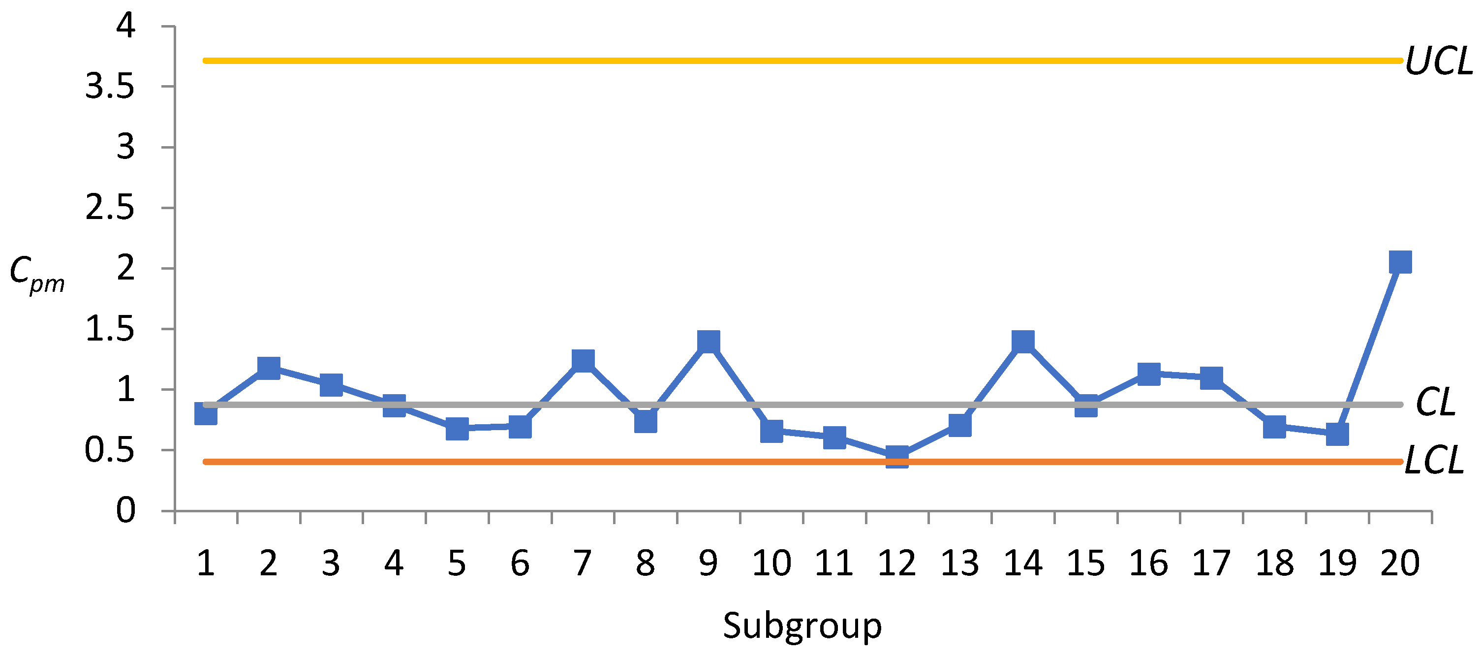
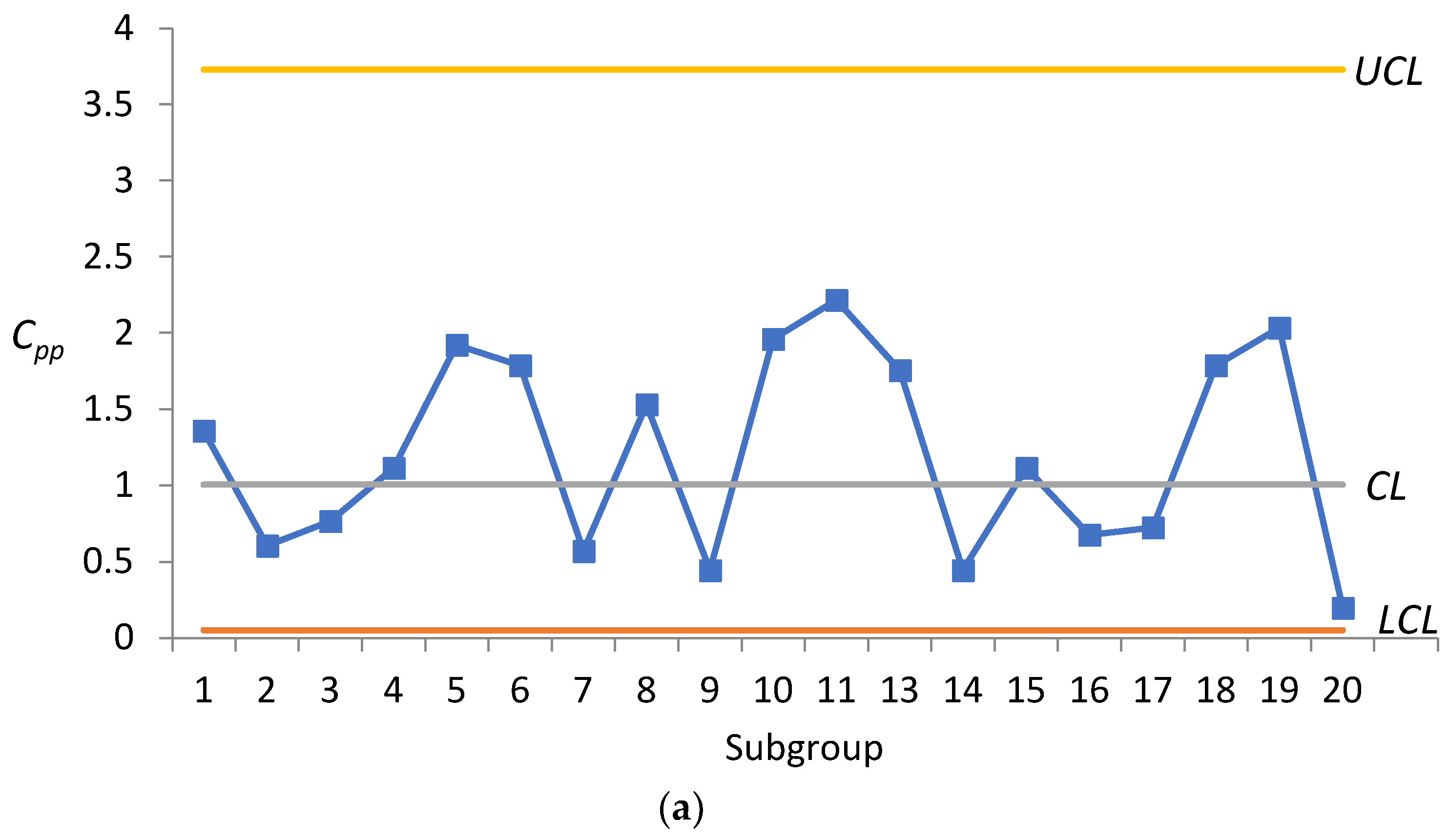
3.2. An Example
- Step 1.
- Collection of data
- Step 2.
- Calculation of , , and
- Step 3.
- Calculation of control limits
- Step 4.
- Plotting the control limits and connecting the dots
- Step 5.
- Breakdown of control charts
- Step 6.
- Breakdown of the process
- Step 7.
- Extension of control limits
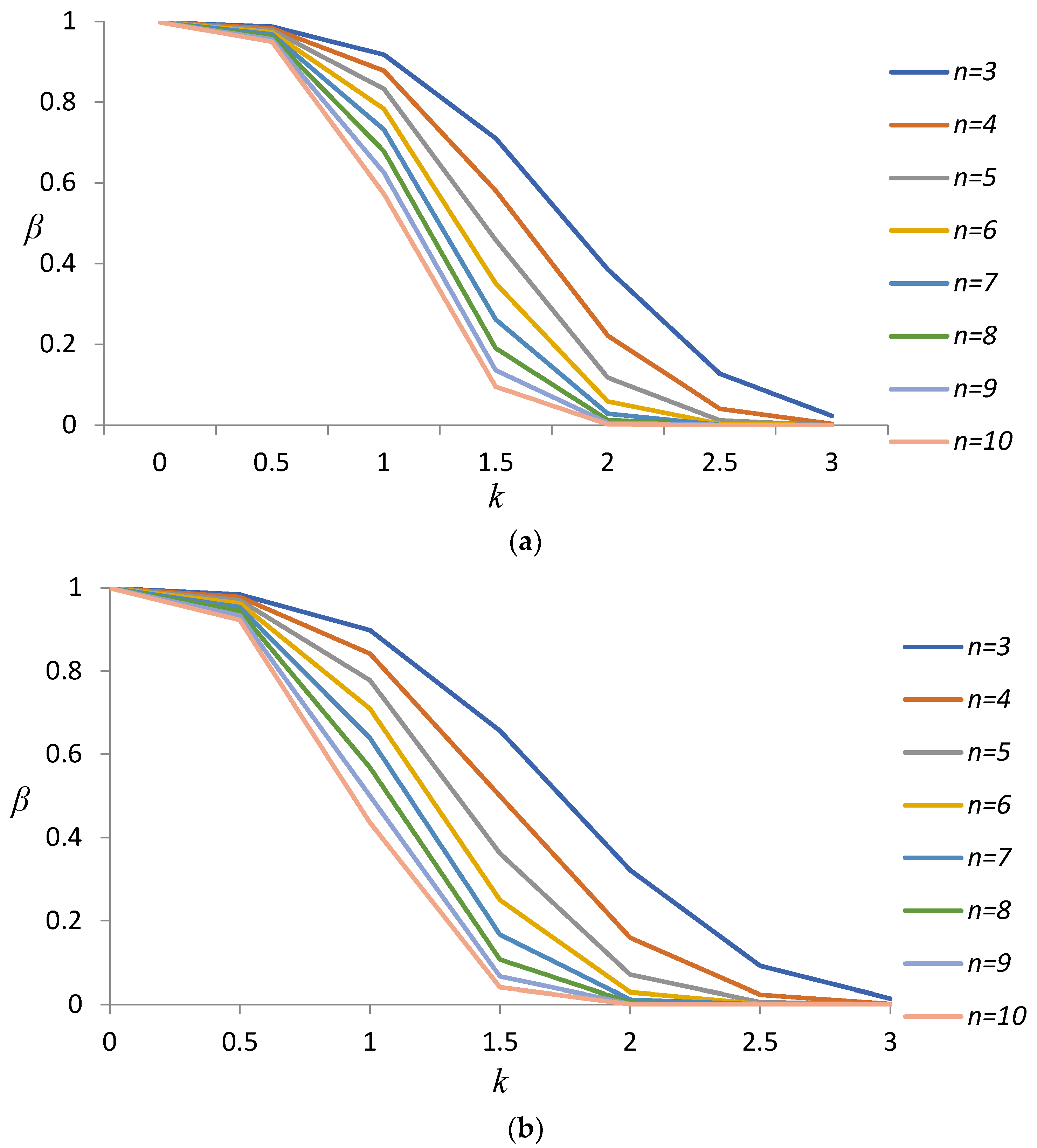
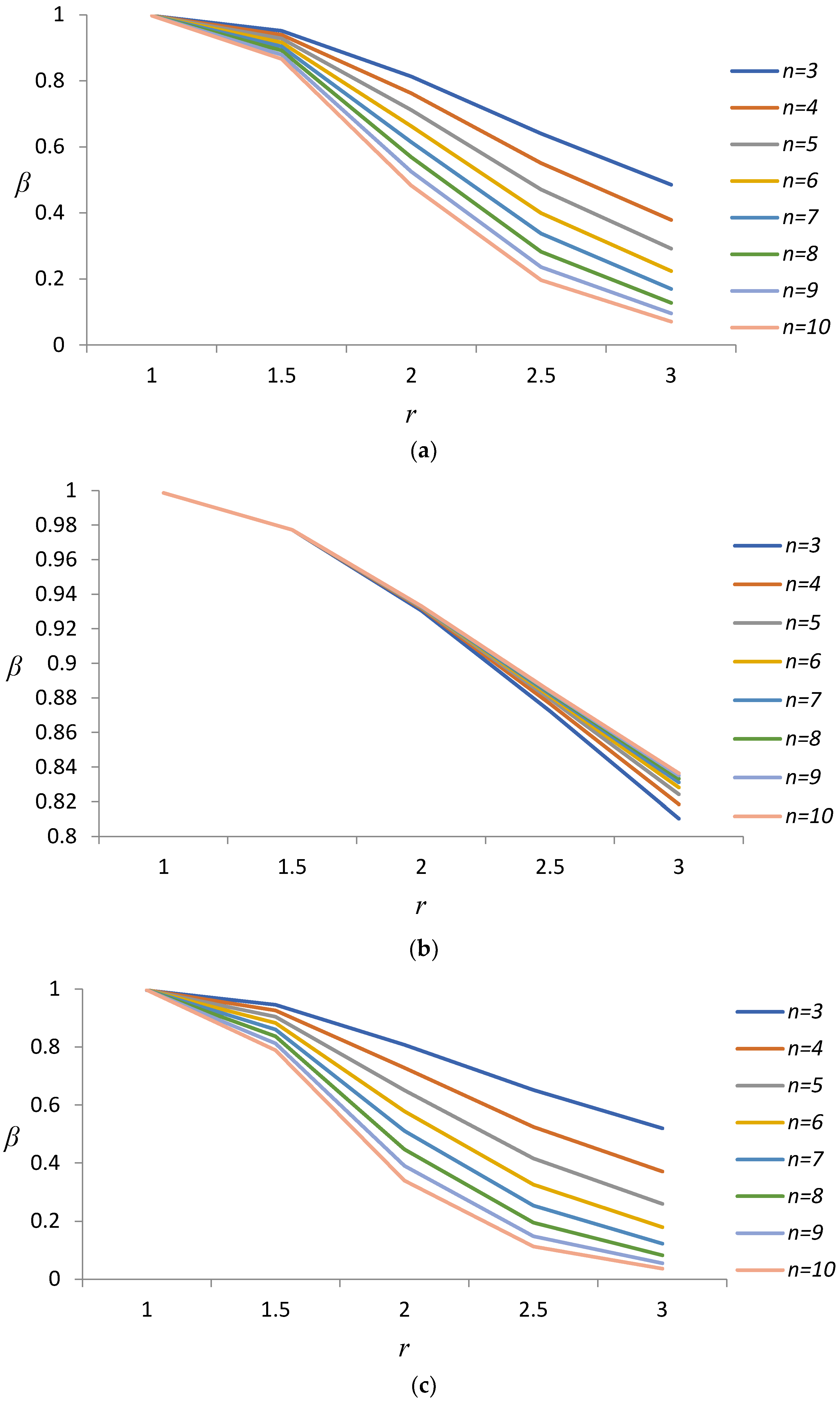
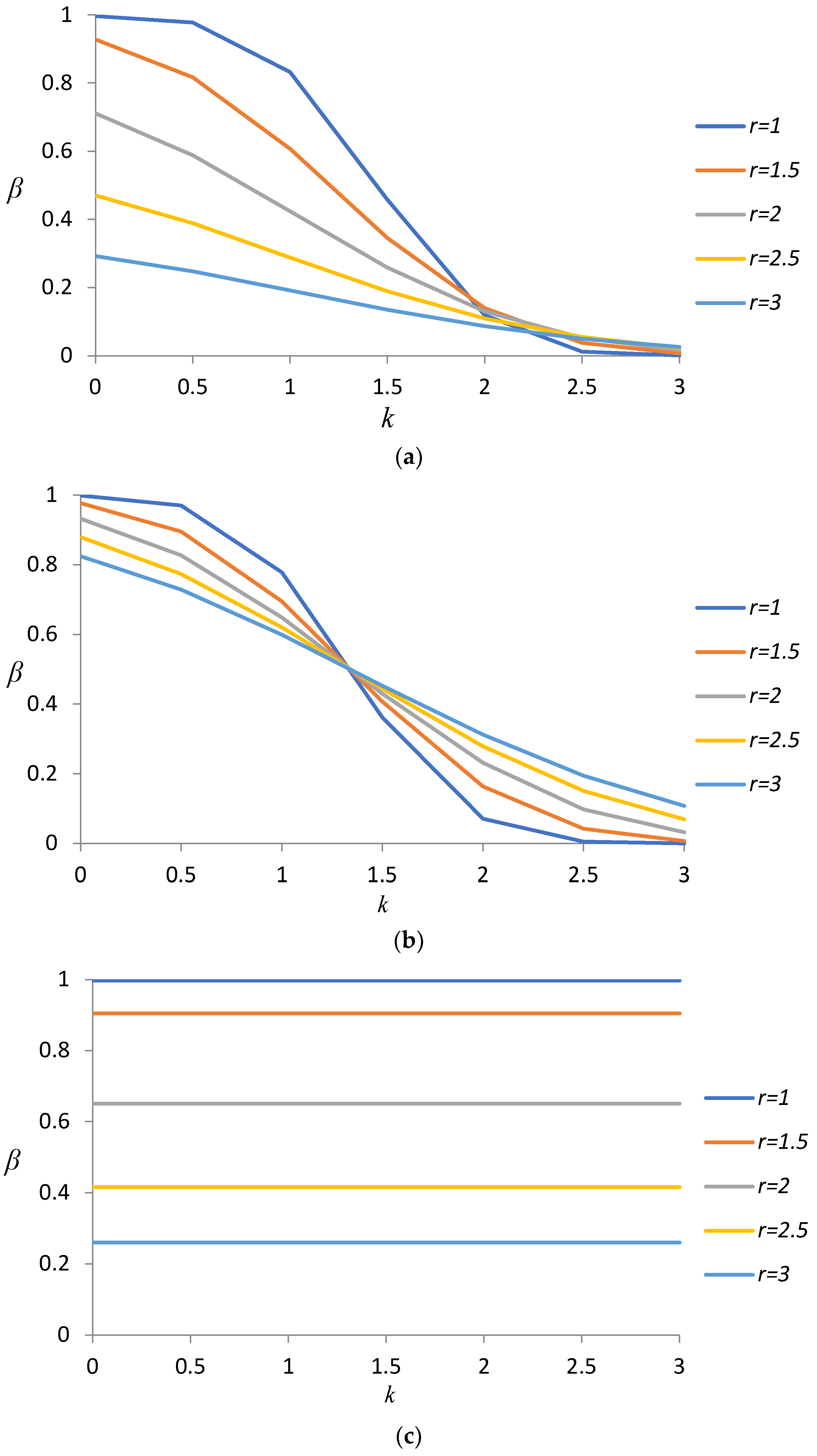
4. Operating Characteristic Curves for Control Charts for , , and
5. Conclusions
Author Contributions
Funding
Data Availability Statement
Conflicts of Interest
References
- Chen, K.S. Estimation of the process incapability index. Commun. Stat. Theory Methods 1998, 27, 1263–1274. [Google Scholar] [CrossRef]
- Chen, K.S. Incapability index with asymmetric tolerances. Stat. Sin. 1998, 8, 253–262. [Google Scholar]
- Davis, R.; Kaminsky, F. Statistical measures of process capability and their relationship to non-conforming products. In Proceedings of the Third Biennial International Manufacturing Technology Research Forum, Chicago, IL, USA, 29–30 August 1989. [Google Scholar]
- Deleryd, M.; Vännman, K. Process capability plots—A quality improvement tool. Qual. Reliab. Eng. Int. 1999, 15, 213–227. [Google Scholar] [CrossRef]
- Chen, K.-S.; Li, F.-C.; Lai, K.-K.; Lin, J.-M. Green Outsourcer Selection Model Based on Confidence Interval of PCI for SMT Process. Sustainability 2022, 14, 16667. [Google Scholar] [CrossRef]
- Boyles, R.A. The Taguchi capability index. J. Qual. Technol. 1991, 23, 17–26. [Google Scholar] [CrossRef]
- Kotz, S.; Johnson, N.L. Process capability indices—A review, 1992–2000. J. Qual. Technol. 2002, 34, 2–19. [Google Scholar] [CrossRef]
- Wu, C.-W.; Pearn, W.; Kotz, S. An overview of theory and practice on process capability indices for quality assurance. Int. J. Prod. Econ. 2009, 117, 338–359. [Google Scholar] [CrossRef]
- Kane, V.E. Process capability indices. J. Qual. Technol. 1986, 18, 41–52. [Google Scholar] [CrossRef]
- Chan, L.K.; Cheng, S.W.; Spiring, F.A. A new measure of process capability: Cpm. J. Qual. Technol. 1988, 20, 162–175. [Google Scholar] [CrossRef]
- Greenwich, M.; Jahr-Schaffrath, B.L. A process incapability index. Int. J. Qual. Reliab. Manag. 1995, 12, 58–71. [Google Scholar] [CrossRef]
- Phillips, G.P. Target ratio simplifies capability index system, makes it easy to use Cpm. Qual. Eng. 1994, 7, 299–313. [Google Scholar] [CrossRef]
- Pearn, W.L.; Chen, K.L.; Chen, K.S. An application of the incapability index Cpp. J. Manag. Syst. 1999, 6, 177–190. [Google Scholar]
- Spiring, F.A. Process capability: A total quality management tool. Total Qual. Manag. 1995, 6, 21–33. [Google Scholar] [CrossRef]
- Castagliola, P. How to monitor capability index Cm using EWMA. Int. J. Reliab. Qual. Saf. Eng. 2001, 8, 191–204. [Google Scholar] [CrossRef]
- Wu, Z.; Xie, M.; Tian, Y. Optimization Design of the &S Charts for Monitoring Process Capability. J. Manuf. Syst. 2002, 21, 83–92. [Google Scholar]
- Chen, K.S.; Huang, H.L.; Huang, C.T. Control Charts for One-sided Capability Indices. Qual. Quant. 2007, 41, 413–427. [Google Scholar] [CrossRef]
- Castagliola, P.; Vännman, K. Monitoring capability indices using EWMA approach. Qual. Reliab. Eng. Int. 2007, 23, 769–790. [Google Scholar] [CrossRef]
- Castagliola, P.; Vännman, K. Average Run Length When Monitoring capability indices using EWMA. Qual. Reliab. Eng. Int. 2008, 24, 941–955. [Google Scholar] [CrossRef]
- Chatterjee, M.; Chakraborty, A.K. Distributions and process capability control charts for Cpu and Cpl using subgroup information. Commun. Stat. Theory Methods 2015, 44, 4333–4353. [Google Scholar] [CrossRef]
- Aslam, M.; Rao, G.S.; AL-Marshadi, A.H.; Ahmad, L.; Jun, C.-H. Control Charts for Monitoring Process Capability Index Using Median Absolute Deviation for Some Popular Distributions. Processes 2019, 7, 287. [Google Scholar] [CrossRef]


| n | 3 | 4 | 5 | 6 | 7 | 8 | 9 | 10 | |||||||||
|---|---|---|---|---|---|---|---|---|---|---|---|---|---|---|---|---|---|
| Constant | |||||||||||||||||
| ξ | 0.0 | 0.072 | 3.116 | 0.121 | 2.786 | 0.166 | 2.567 | 0.206 | 2.408 | 0.241 | 2.288 | 0.272 | 2.192 | 0.300 | 2.114 | 0.325 | 2.060 |
| 0.1 | 0.072 | 3.105 | 0.122 | 2.776 | 0.167 | 2.558 | 0.207 | 2.400 | 0.242 | 2.280 | 0.273 | 2.185 | 0.301 | 2.107 | 0.326 | 2.054 | |
| 0.2 | 0.073 | 3.077 | 0.123 | 2.752 | 0.169 | 2.537 | 0.209 | 2.381 | 0.245 | 2.263 | 0.276 | 2.169 | 0.304 | 2.093 | 0.329 | 2.040 | |
| 0.3 | 0.075 | 3.040 | 0.125 | 2.721 | 0.172 | 2.510 | 0.212 | 2.357 | 0.248 | 2.241 | 0.28 | 2.149 | 0.308 | 2.074 | 0.333 | 2.022 | |
| 0.4 | 0.076 | 2.999 | 0.128 | 2.687 | 0.175 | 2.480 | 0.217 | 2.330 | 0.253 | 2.217 | 0.285 | 2.127 | 0.313 | 2.053 | 0.338 | 2.002 | |
| 0.5 | 0.078 | 2.957 | 0.131 | 2.651 | 0.179 | 2.448 | 0.221 | 2.303 | 0.258 | 2.192 | 0.290 | 2.104 | 0.318 | 2.032 | 0.343 | 1.982 | |
| 0.6 | 0.081 | 2.914 | 0.135 | 2.615 | 0.184 | 2.417 | 0.227 | 2.275 | 0.264 | 2.166 | 0.296 | 2.080 | 0.324 | 2.010 | 0.350 | 1.961 | |
| 0.7 | 0.084 | 2.872 | 0.139 | 2.58 | 0.189 | 2.387 | 0.232 | 2.248 | 0.27 | 2.142 | 0.302 | 2.058 | 0.331 | 1.989 | 0.356 | 1.941 | |
| 0.8 | 0.087 | 2.831 | 0.144 | 2.546 | 0.195 | 2.357 | 0.238 | 2.221 | 0.276 | 2.118 | 0.309 | 2.036 | 0.338 | 1.969 | 0.363 | 1.922 | |
| 0.9 | 0.090 | 2.791 | 0.149 | 2.513 | 0.200 | 2.329 | 0.245 | 2.196 | 0.283 | 2.095 | 0.316 | 2.015 | 0.344 | 1.949 | 0.370 | 1.903 | |
| 1.0 | 0.094 | 2.754 | 0.154 | 2.481 | 0.207 | 2.301 | 0.251 | 2.172 | 0.290 | 2.073 | 0.323 | 1.994 | 0.351 | 1.930 | 0.377 | 1.885 | |
| n | 3 | 4 | 5 | 6 | 7 | 8 | 9 | 10 | |||||||||
|---|---|---|---|---|---|---|---|---|---|---|---|---|---|---|---|---|---|
| Constants | |||||||||||||||||
| ξ | 0.0 | 0.038 | 3.782 | 0.074 | 3.319 | 0.111 | 3.017 | 0.145 | 2.802 | 0.177 | 2.639 | 0.206 | 2.511 | 0.232 | 2.407 | 0.256 | 2.321 |
| 0.1 | 0.038 | 3.762 | 0.075 | 3.303 | 0.111 | 3.003 | 0.146 | 2.790 | 0.178 | 2.628 | 0.207 | 2.501 | 0.233 | 2.398 | 0.257 | 2.312 | |
| 0.2 | 0.039 | 3.717 | 0.076 | 3.266 | 0.113 | 2.972 | 0.148 | 2.762 | 0.180 | 2.603 | 0.209 | 2.479 | 0.235 | 2.377 | 0.259 | 2.293 | |
| 0.3 | 0.040 | 3.661 | 0.077 | 3.219 | 0.115 | 2.932 | 0.150 | 2.727 | 0.182 | 2.572 | 0.212 | 2.450 | 0.239 | 2.351 | 0.263 | 2.268 | |
| 0.4 | 0.041 | 3.599 | 0.079 | 3.169 | 0.117 | 2.889 | 0.153 | 2.689 | 0.186 | 2.538 | 0.216 | 2.419 | 0.243 | 2.322 | 0.267 | 2.242 | |
| 0.5 | 0.042 | 3.535 | 0.081 | 3.117 | 0.120 | 2.844 | 0.157 | 2.650 | 0.190 | 2.503 | 0.221 | 2.387 | 0.248 | 2.293 | 0.273 | 2.215 | |
| 0.6 | 0.043 | 3.473 | 0.084 | 3.066 | 0.124 | 2.801 | 0.161 | 2.612 | 0.195 | 2.468 | 0.226 | 2.356 | 0.253 | 2.264 | 0.278 | 2.188 | |
| 0.7 | 0.045 | 3.413 | 0.086 | 3.017 | 0.128 | 2.759 | 0.166 | 2.574 | 0.200 | 2.435 | 0.231 | 2.325 | 0.259 | 2.236 | 0.284 | 2.161 | |
| 0.8 | 0.047 | 3.354 | 0.090 | 2.969 | 0.132 | 2.718 | 0.171 | 2.538 | 0.206 | 2.403 | 0.237 | 2.296 | 0.265 | 2.208 | 0.291 | 2.136 | |
| 0.9 | 0.049 | 3.299 | 0.093 | 2.924 | 0.136 | 2.679 | 0.176 | 2.504 | 0.212 | 2.372 | 0.243 | 2.267 | 0.272 | 2.182 | 0.297 | 2.112 | |
| 1.0 | 0.051 | 3.246 | 0.097 | 2.881 | 0.141 | 2.642 | 0.182 | 2.471 | 0.218 | 2.342 | 0.250 | 2.240 | 0.278 | 2.157 | 0.304 | 2.088 | |
| n | 3 | 4 | 5 | 6 | 7 | 8 | 9 | 10 | |||||||||
|---|---|---|---|---|---|---|---|---|---|---|---|---|---|---|---|---|---|
| Constants | |||||||||||||||||
| ξ | 0.0 | 0.000 | 1.675 | 0.000 | 1.256 | 0.000 | 1.005 | 0.000 | 0.837 | 0.000 | 0.718 | 0.000 | 0.628 | 0.000 | 0.558 | 0.000 | 0.502 |
| 0.1 | 0.000 | 2.127 | 0.000 | 1.694 | 0.000 | 1.429 | 0.000 | 1.250 | 0.000 | 1.119 | 0.000 | 1.020 | 0.000 | 0.941 | 0.000 | 0.877 | |
| 0.2 | 0.001 | 2.500 | 0.001 | 2.039 | 0.001 | 1.753 | 0.001 | 1.556 | 0.001 | 1.411 | 0.001 | 1.300 | 0.001 | 1.211 | 0.001 | 1.139 | |
| 0.3 | 0.001 | 2.822 | 0.001 | 2.334 | 0.001 | 2.029 | 0.001 | 1.817 | 0.001 | 1.660 | 0.001 | 1.539 | 0.002 | 1.443 | 0.002 | 1.363 | |
| 0.4 | 0.001 | 3.112 | 0.001 | 2.600 | 0.001 | 2.277 | 0.002 | 2.052 | 0.002 | 1.886 | 0.003 | 1.757 | 0.004 | 1.653 | 0.005 | 1.568 | |
| 0.5 | 0.001 | 3.381 | 0.002 | 2.846 | 0.002 | 2.508 | 0.003 | 2.272 | 0.005 | 2.096 | 0.006 | 1.960 | 0.009 | 1.851 | 0.012 | 1.761 | |
| 0.6 | 0.002 | 3.634 | 0.003 | 3.079 | 0.004 | 2.726 | 0.006 | 2.480 | 0.009 | 2.296 | 0.013 | 2.154 | 0.019 | 2.039 | 0.027 | 1.944 | |
| 0.7 | 0.003 | 3.874 | 0.004 | 3.300 | 0.006 | 2.935 | 0.010 | 2.679 | 0.016 | 2.488 | 0.025 | 2.340 | 0.036 | 2.220 | 0.048 | 2.121 | |
| 0.8 | 0.004 | 4.105 | 0.006 | 3.513 | 0.010 | 3.136 | 0.017 | 2.872 | 0.029 | 2.674 | 0.043 | 2.520 | 0.059 | 2.396 | 0.076 | 2.293 | |
| 0.9 | 0.005 | 4.328 | 0.009 | 3.720 | 0.016 | 3.331 | 0.029 | 3.058 | 0.046 | 2.854 | 0.066 | 2.695 | 0.088 | 2.566 | 0.108 | 2.460 | |
| 1.0 | 0.006 | 4.544 | 0.013 | 3.920 | 0.025 | 3.521 | 0.044 | 3.241 | 0.069 | 3.030 | 0.095 | 2.866 | 0.120 | 2.733 | 0.145 | 2.624 | |
| n | 3 | 4 | 5 | 6 | 7 | 8 | 9 | 10 | |||||||||
|---|---|---|---|---|---|---|---|---|---|---|---|---|---|---|---|---|---|
| Constants | |||||||||||||||||
| ξ | 0.0 | 0.000 | 3.609 | 0.000 | 2.707 | 0.000 | 2.166 | 0.000 | 1.805 | 0.000 | 1.547 | 0.000 | 1.353 | 0.000 | 1.203 | 0.000 | 1.083 |
| 0.1 | 0.000 | 4.422 | 0.000 | 3.468 | 0.000 | 2.885 | 0.000 | 2.490 | 0.000 | 2.203 | 0.000 | 1.985 | 0.000 | 1.813 | 0.000 | 1.673 | |
| 0.2 | 0.000 | 4.980 | 0.000 | 3.970 | 0.000 | 3.346 | 0.000 | 2.920 | 0.000 | 2.609 | 0.000 | 2.371 | 0.000 | 2.182 | 0.000 | 2.029 | |
| 0.3 | 0.000 | 5.438 | 0.000 | 4.380 | 0.000 | 3.724 | 0.000 | 3.274 | 0.000 | 2.944 | 0.000 | 2.691 | 0.000 | 2.489 | 0.000 | 2.325 | |
| 0.4 | 0.000 | 5.840 | 0.000 | 4.742 | 0.000 | 4.058 | 0.000 | 3.587 | 0.000 | 3.242 | 0.000 | 2.976 | 0.000 | 2.764 | 0.000 | 2.591 | |
| 0.5 | 0.000 | 6.206 | 0.000 | 5.073 | 0.000 | 4.364 | 0.000 | 3.876 | 0.000 | 3.516 | 0.000 | 3.239 | 0.000 | 3.018 | 0.000 | 2.837 | |
| 0.6 | 0.000 | 6.547 | 0.000 | 5.381 | 0.000 | 4.651 | 0.000 | 4.146 | 0.000 | 3.774 | 0.000 | 3.486 | 0.000 | 3.257 | 0.000 | 3.069 | |
| 0.7 | 0.000 | 6.869 | 0.000 | 5.673 | 0.000 | 4.922 | 0.000 | 4.403 | 0.000 | 4.019 | 0.000 | 3.722 | 0.000 | 3.485 | 0.000 | 3.290 | |
| 0.8 | 0.000 | 7.175 | 0.000 | 5.951 | 0.000 | 5.182 | 0.000 | 4.648 | 0.000 | 4.254 | 0.000 | 3.948 | 0.000 | 3.704 | 0.000 | 3.503 | |
| 0.9 | 0.000 | 7.468 | 0.000 | 6.219 | 0.000 | 5.432 | 0.000 | 4.885 | 0.000 | 4.480 | 0.000 | 4.167 | 0.001 | 3.915 | 0.001 | 3.709 | |
| 1.0 | 0.000 | 7.751 | 0.000 | 6.478 | 0.000 | 5.674 | 0.000 | 5.115 | 0.000 | 4.700 | 0.001 | 4.379 | 0.001 | 4.121 | 0.003 | 3.909 | |
| n | 3 | 4 | 5 | 6 | 7 | 8 | 9 | 10 | |||||||||
|---|---|---|---|---|---|---|---|---|---|---|---|---|---|---|---|---|---|
| Constants | |||||||||||||||||
| 0.017 | 2.459 | 0.054 | 2.337 | 0.097 | 2.229 | 0.139 | 2.139 | 0.177 | 2.064 | 0.211 | 2.002 | 0.242 | 1.948 | 0.270 | 1.902 | ||
| n | 3 | 4 | 5 | 6 | 7 | 8 | 9 | 10 | |||||||||
|---|---|---|---|---|---|---|---|---|---|---|---|---|---|---|---|---|---|
| Constants | |||||||||||||||||
| 0.001 | 4.605 | 0.006 | 4.067 | 0.018 | 3.693 | 0.035 | 3.419 | 0.054 | 3.208 | 0.075 | 3.040 | 0.095 | 2.903 | 0.115 | 2.788 | ||
| Subgroup | Observations | |||||||
|---|---|---|---|---|---|---|---|---|
| 1 | X11 | X12 | ···X1n | |||||
| 2 | X21 | X22 | ···X2n | |||||
| · | · | ····· | · | · | · | · | · | |
| · | · | ····· | · | · | · | · | · | |
| · | · | ····· | · | · | · | · | · | |
| m | Xm1 | Xm2 | ···Xmn | |||||
| Index | Control Limit | Process Evaluation Criteria |
|---|---|---|
| 1. , the process capability is poor. 2. , the process s is typically called capable. 3. , the process s is typically called satisfactory. 4. , the process s is typically called good. 5. , the process s is typically called super. | ||
| , the process accuracy is good. | ||
| 1. 1.00, the process precision is capable. 2. 0.56, the process precision is satisfactory. 3. 0.44, the process precision is good. 4. 0.36, the process precision is excellent. 5. 0.25, the process precision is super. |
| Subgroup | Observations | S | |||||||||
|---|---|---|---|---|---|---|---|---|---|---|---|
| 1 | 1.81 | 2.21 | 2.06 | 1.96 | 2.11 | 2.030 | 0.1525 | 0.0506 | 1.3078 | 1.3584 | 0.8049 |
| 2 | 2.01 | 2.15 | 1.97 | 2.12 | 2.10 | 2.070 | 0.0765 | 0.2756 | 0.3291 | 0.6047 | 1.1810 |
| 3 | 2.16 | 2.17 | 2.00 | 2.04 | 2.08 | 2.090 | 0.0742 | 0.4556 | 0.3094 | 0.7650 | 1.0428 |
| 4 | 2.12 | 2.09 | 2.25 | 2.05 | 1.97 | 2.096 | 0.1029 | 0.5184 | 0.5951 | 1.1135 | 0.8699 |
| 5 | 2.15 | 2.11 | 1.76 | 1.82 | 2.11 | 1.990 | 0.1845 | 0.0056 | 1.9153 | 1.9209 | 0.6781 |
| 6 | 2.22 | 1.93 | 2.08 | 2.27 | 1.95 | 2.090 | 0.1538 | 0.4556 | 1.3303 | 1.7859 | 0.6942 |
| 7 | 1.98 | 2.19 | 2.02 | 1.96 | 1.95 | 2.020 | 0.0987 | 0.0225 | 0.5484 | 0.5709 | 1.2415 |
| 8 | 2.08 | 2.11 | 2.28 | 1.95 | 2.15 | 2.114 | 0.1193 | 0.7310 | 0.8004 | 1.5315 | 0.7413 |
| 9 | 2.01 | 2.05 | 2.11 | 2.10 | 1.91 | 2.036 | 0.0811 | 0.0729 | 0.3701 | 0.4430 | 1.4003 |
| 10 | 2.06 | 2.24 | 2.29 | 1.93 | 2.00 | 2.104 | 0.1550 | 0.6084 | 1.3517 | 1.9601 | 0.6608 |
| 11 | 2.29 | 2.25 | 2.11 | 2.09 | 2.15 | 2.178 | 0.0879 | 1.7822 | 0.4343 | 2.2165 | 0.6064 |
| 12 | 1.91 | 1.95 | 2.38 | 2.40 | 1.94 | 2.116 | 0.2507 | 0.7569 | 3.5342 | 4.2911 | 0.4497 |
| 13 | 2.22 | 2.20 | 2.05 | 1.98 | 1.81 | 2.052 | 0.1687 | 0.1521 | 1.6014 | 1.7535 | 0.7067 |
| 14 | 2.01 | 2.05 | 2.11 | 2.10 | 1.91 | 2.036 | 0.0811 | 0.0729 | 0.3701 | 0.4430 | 1.4003 |
| 15 | 2.12 | 2.09 | 2.25 | 2.05 | 1.97 | 2.096 | 0.1029 | 0.5184 | 0.5951 | 1.1135 | 0.8699 |
| 16 | 2.18 | 1.96 | 2.12 | 1.97 | 2.04 | 2.054 | 0.0953 | 0.1640 | 0.5108 | 0.6748 | 1.1301 |
| 17 | 2.16 | 2.04 | 2.13 | 1.91 | 1.97 | 2.042 | 0.1052 | 0.0992 | 0.6227 | 0.7219 | 1.0985 |
| 18 | 2.22 | 1.93 | 2.08 | 2.27 | 1.95 | 2.090 | 0.1538 | 0.4556 | 1.3303 | 1.7859 | 0.6942 |
| 19 | 2.18 | 2.20 | 2.07 | 2.29 | 2.11 | 2.170 | 0.0851 | 1.6256 | 0.4078 | 2.0334 | 0.6333 |
| 20 | 2.06 | 2.05 | 1.97 | 2.05 | 2.08 | 2.042 | 0.0421 | 0.0992 | 0.0996 | 0.1988 | 2.0554 |
Disclaimer/Publisher’s Note: The statements, opinions and data contained in all publications are solely those of the individual author(s) and contributor(s) and not of MDPI and/or the editor(s). MDPI and/or the editor(s) disclaim responsibility for any injury to people or property resulting from any ideas, methods, instructions or products referred to in the content. |
© 2023 by the authors. Licensee MDPI, Basel, Switzerland. This article is an open access article distributed under the terms and conditions of the Creative Commons Attribution (CC BY) license (https://creativecommons.org/licenses/by/4.0/).
Share and Cite
Kuo, T.-I.; Chuang, T.-L. Process Capability Control Charts for Monitoring Process Accuracy and Precision. Axioms 2023, 12, 857. https://doi.org/10.3390/axioms12090857
Kuo T-I, Chuang T-L. Process Capability Control Charts for Monitoring Process Accuracy and Precision. Axioms. 2023; 12(9):857. https://doi.org/10.3390/axioms12090857
Chicago/Turabian StyleKuo, Tsen-I, and Tung-Lin Chuang. 2023. "Process Capability Control Charts for Monitoring Process Accuracy and Precision" Axioms 12, no. 9: 857. https://doi.org/10.3390/axioms12090857
APA StyleKuo, T.-I., & Chuang, T.-L. (2023). Process Capability Control Charts for Monitoring Process Accuracy and Precision. Axioms, 12(9), 857. https://doi.org/10.3390/axioms12090857