Author Contributions
Conceptualization, O.H.O., H.M.A. and Z.A.; methodology, O.H.O., H.M.A. and Z.A.; software, H.M.A., Z.A. and G.S.R.; validation, O.H.O. and Z.A.; formal analysis, O.H.O., H.M.A., Z.A. and G.S.R.; investigation, O.H.O.; data curation, Z.A. and G.S.R.; writing—original draft preparation, O.H.O., H.M.A., Z.A. and G.S.R.; writing—review and editing, O.H.O., H.M.A. and Z.A.; visualization, O.H.O., Z.A. and G.S.R. All authors have read and agreed to the published version of the manuscript.
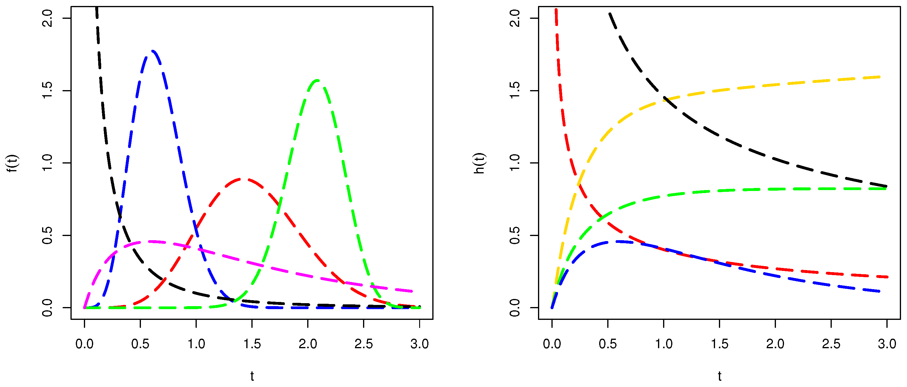
Figure 1.
The plots of and of the WC-Weibull model for different values of and .
Figure 1.
The plots of and of the WC-Weibull model for different values of and .
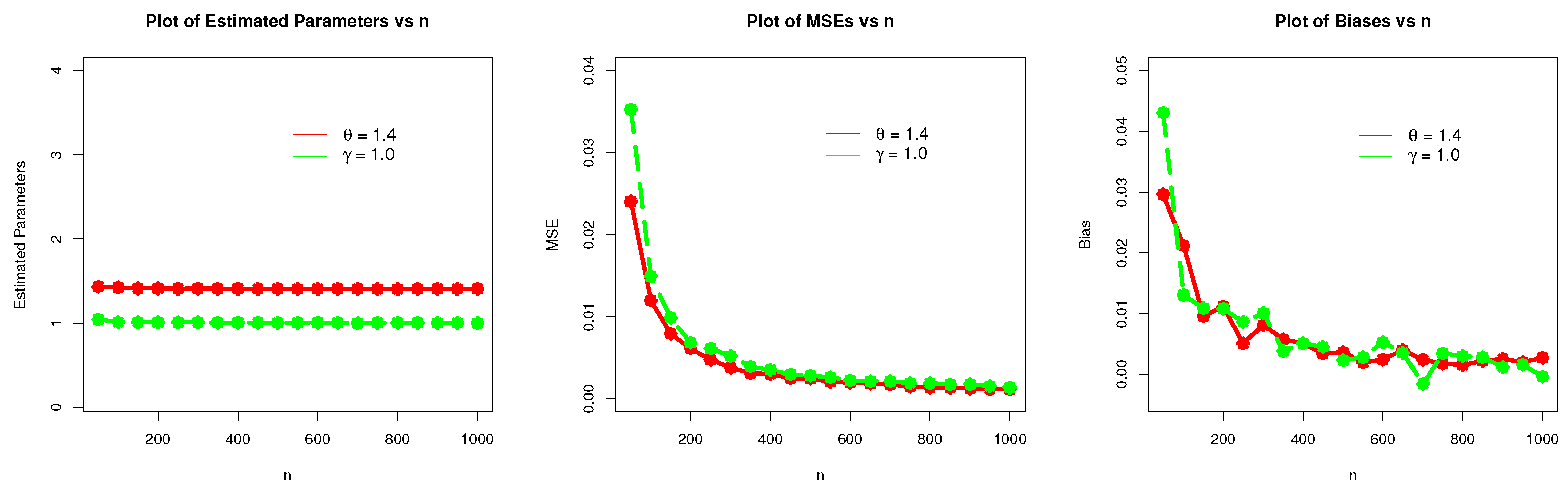
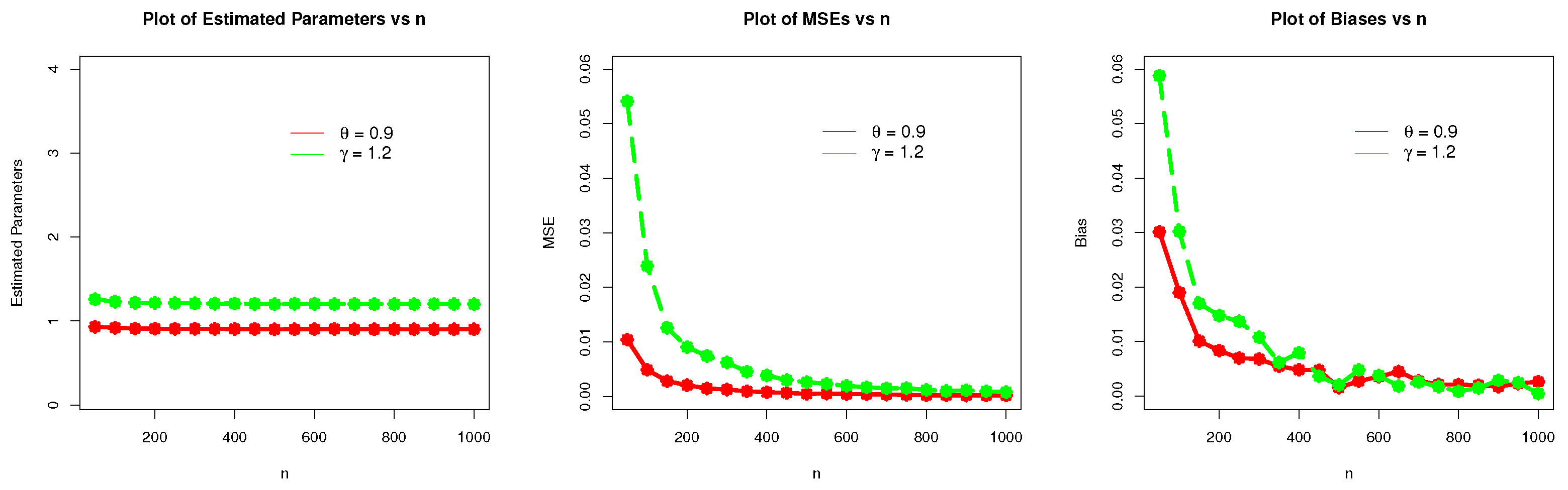
Figure 2.
The simulation results (visual illustration) of the WC-Weibull distribution for and .
Figure 2.
The simulation results (visual illustration) of the WC-Weibull distribution for and .
Figure 3.
The simulation results (visual illustration) of the WC-Weibull distribution for and .
Figure 3.
The simulation results (visual illustration) of the WC-Weibull distribution for and .
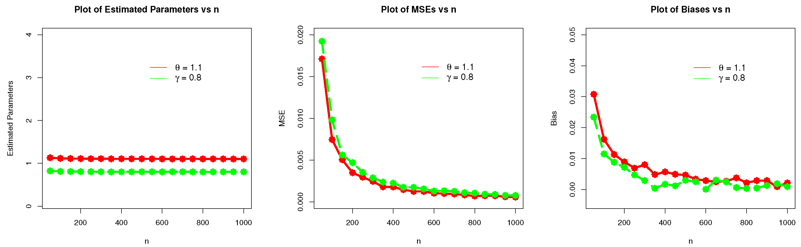
Figure 4.
The simulation results (visual illustration) of the WC-Weibull distribution for and .
Figure 4.
The simulation results (visual illustration) of the WC-Weibull distribution for and .
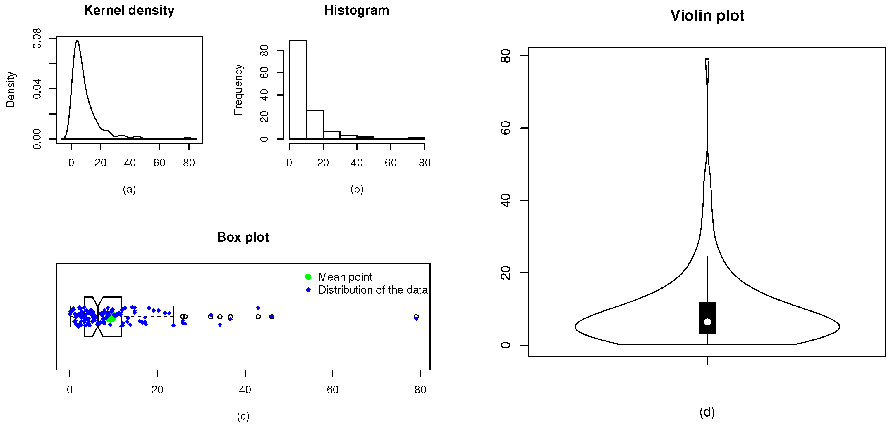
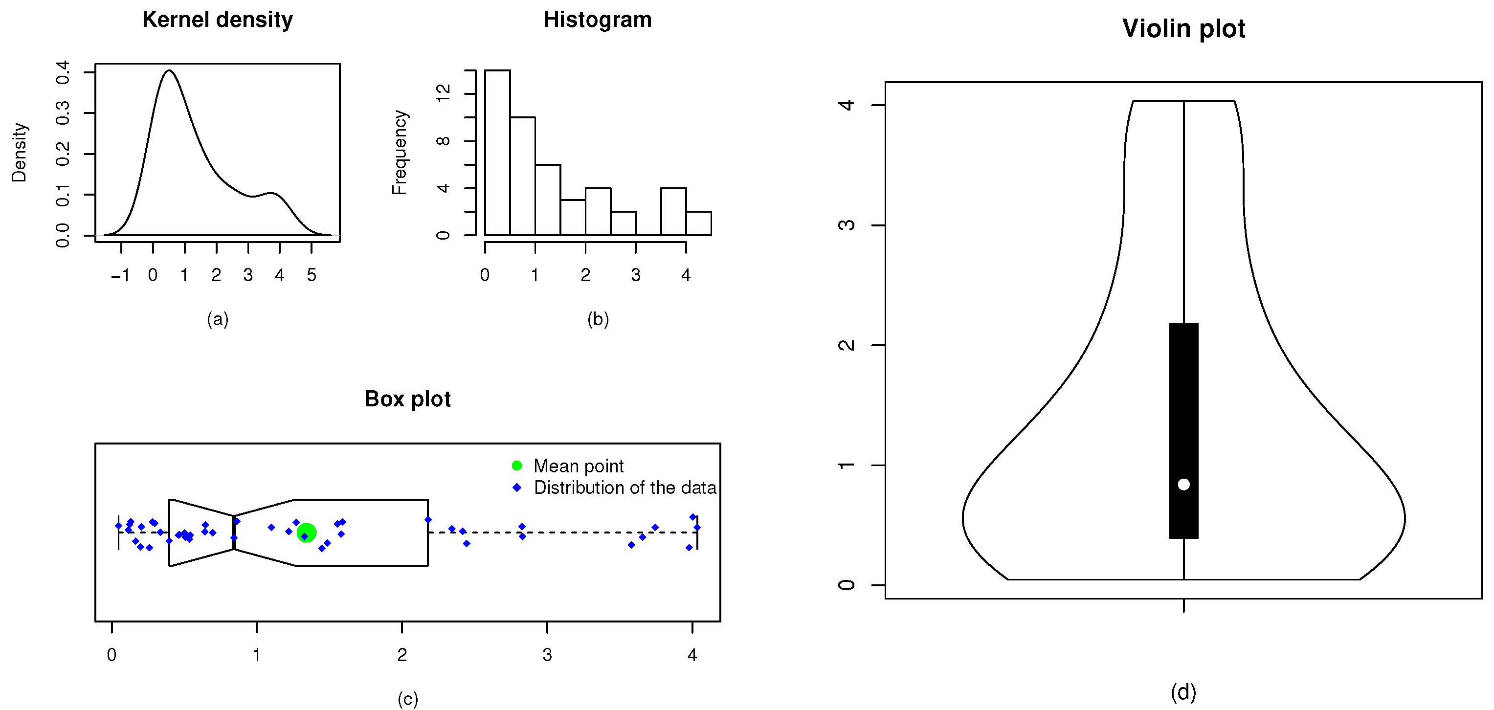
Figure 5.
The kernel density (a), histogram (b), box plot (c), and violin plot (d) of Data 1.
Figure 5.
The kernel density (a), histogram (b), box plot (c), and violin plot (d) of Data 1.
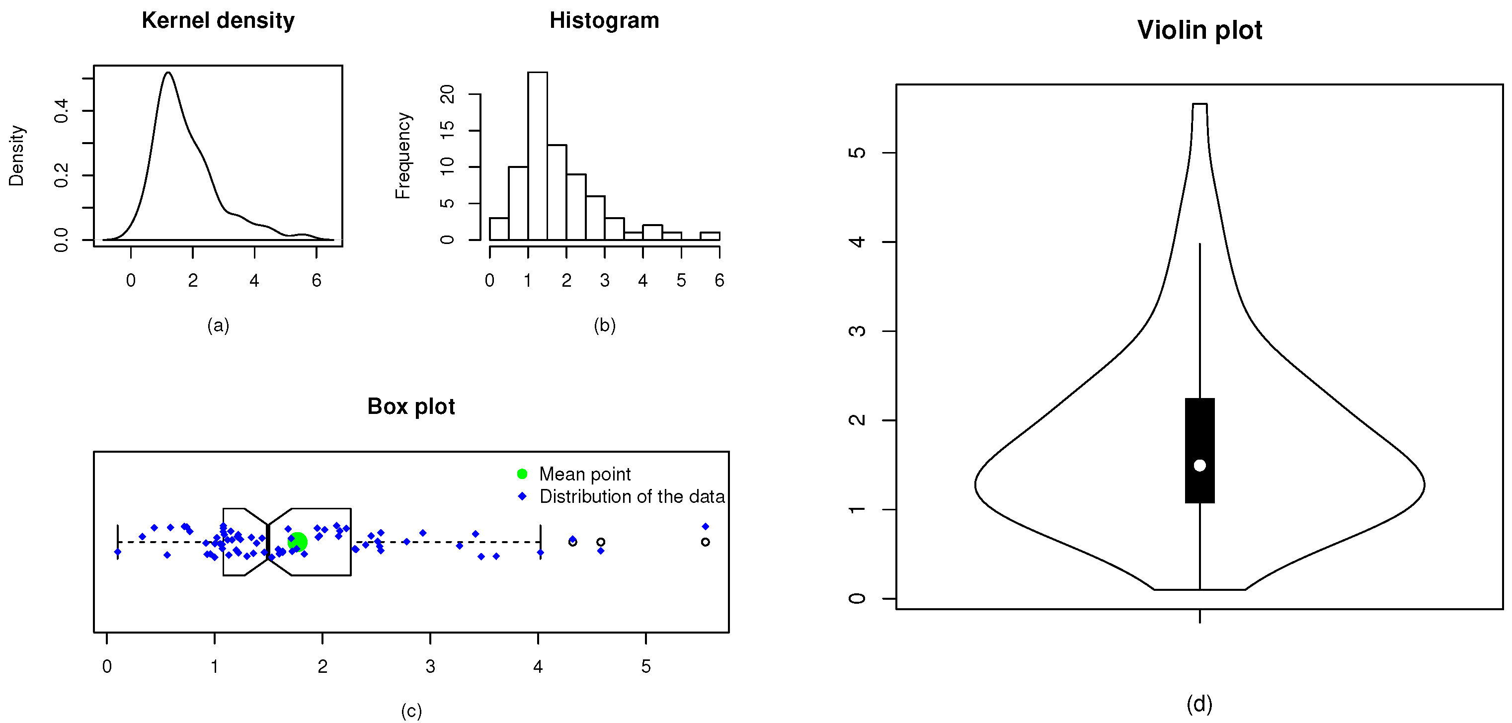
Figure 6.
The kernel density (a), histogram (b), box plot (c), and violin plot (d) of Data 2.
Figure 6.
The kernel density (a), histogram (b), box plot (c), and violin plot (d) of Data 2.
Figure 7.
The kernel density (a), histogram (b), box plot (c), and violin plot (d) of Data 3.
Figure 7.
The kernel density (a), histogram (b), box plot (c), and violin plot (d) of Data 3.
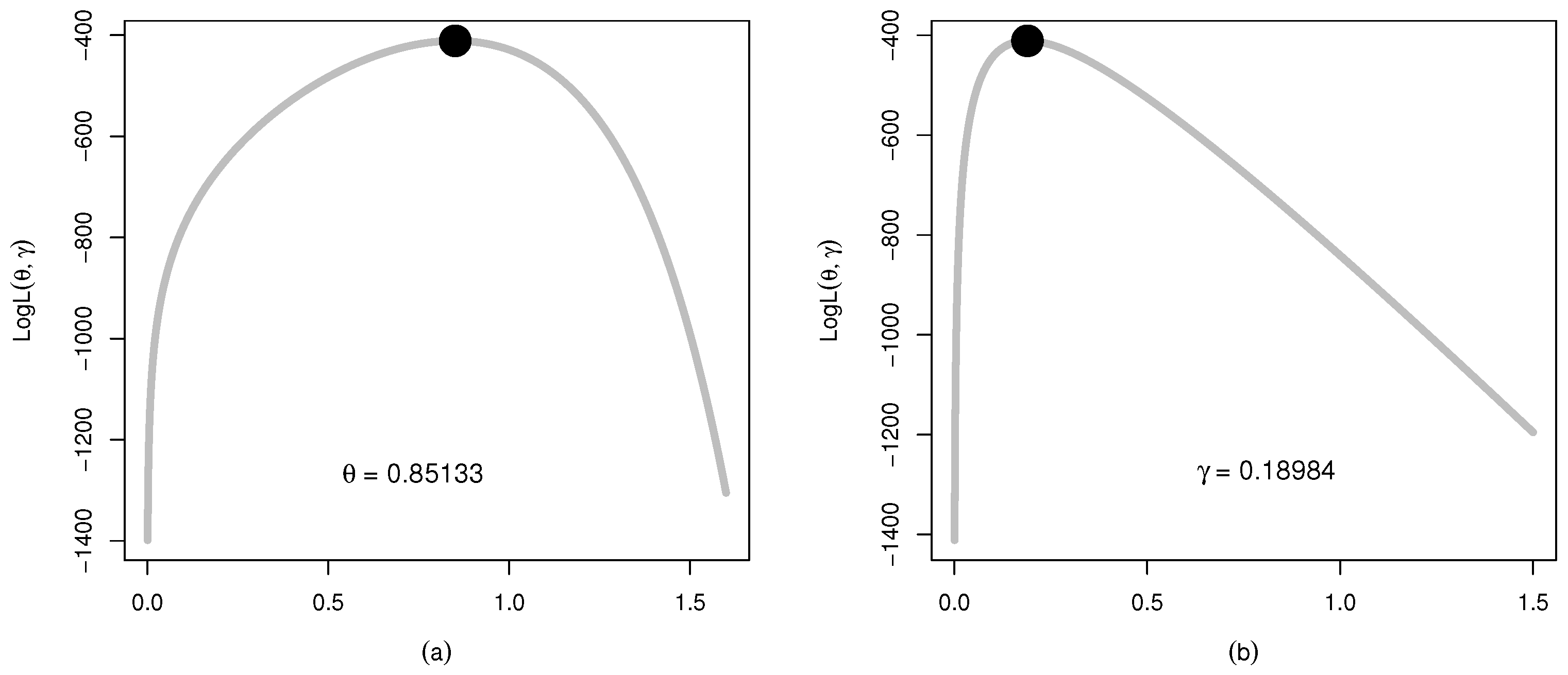
Figure 8.
The plots for the (a) log-likelihood profile of and (b) log-likelihood profile of of the WC-Weibull distribution for Data 1.
Figure 8.
The plots for the (a) log-likelihood profile of and (b) log-likelihood profile of of the WC-Weibull distribution for Data 1.
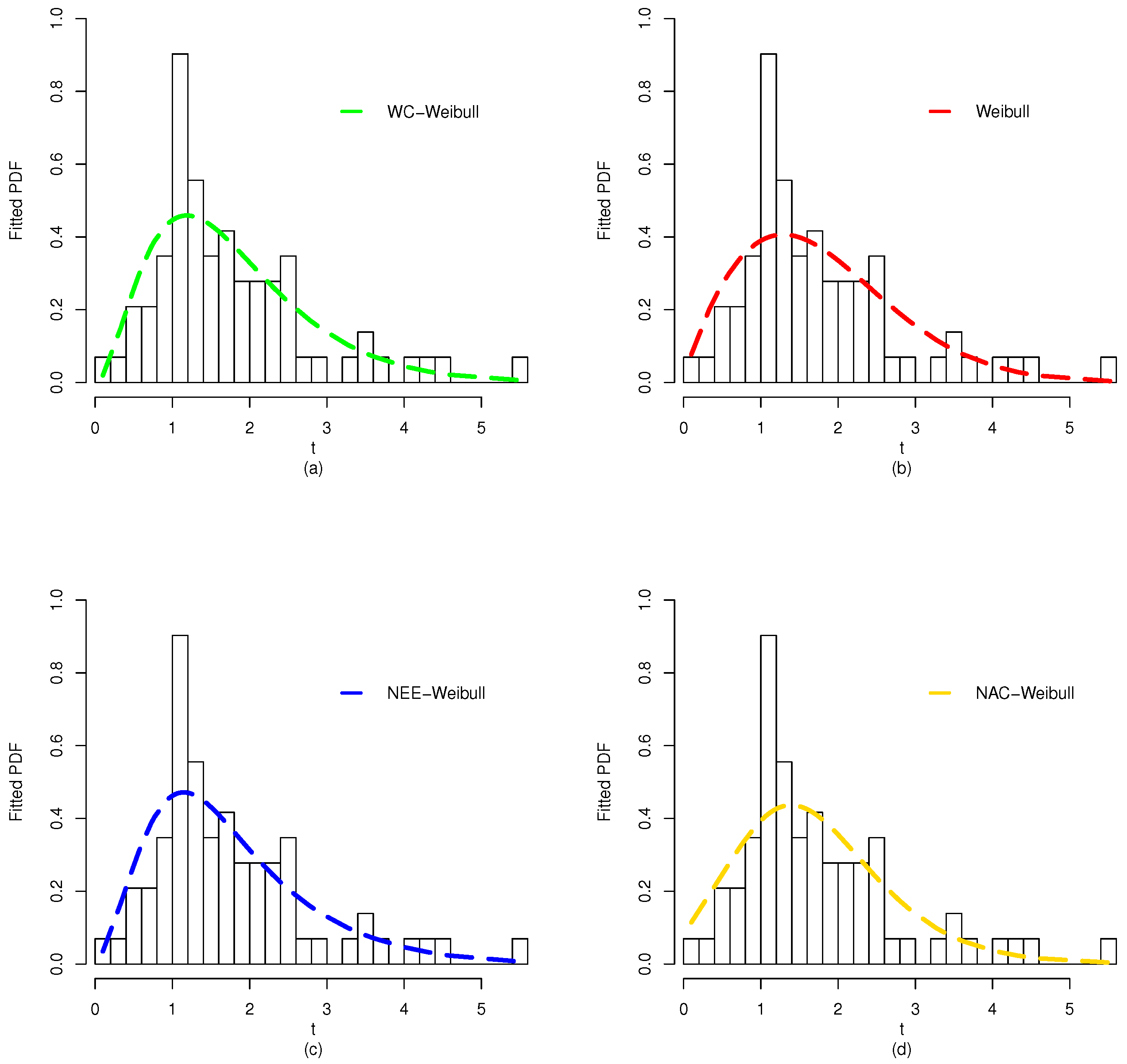
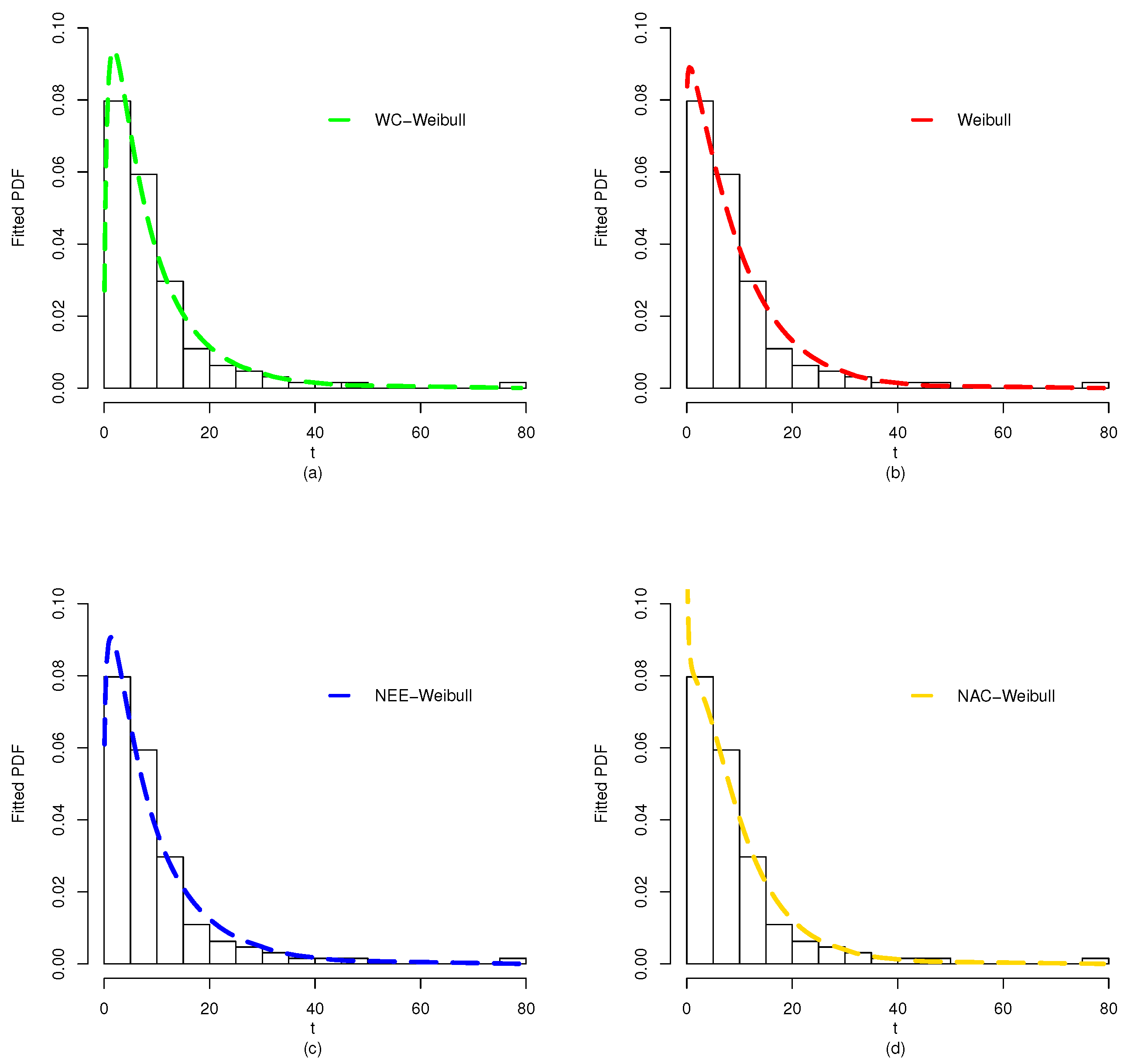
Figure 9.
The plots for the fitted PDF of (a) WC-Weibull distribution, (b) Weibull distribution, (c) NEE-Weibull distribution, and (d) NAC-Weibull distribution for Data 1.
Figure 9.
The plots for the fitted PDF of (a) WC-Weibull distribution, (b) Weibull distribution, (c) NEE-Weibull distribution, and (d) NAC-Weibull distribution for Data 1.
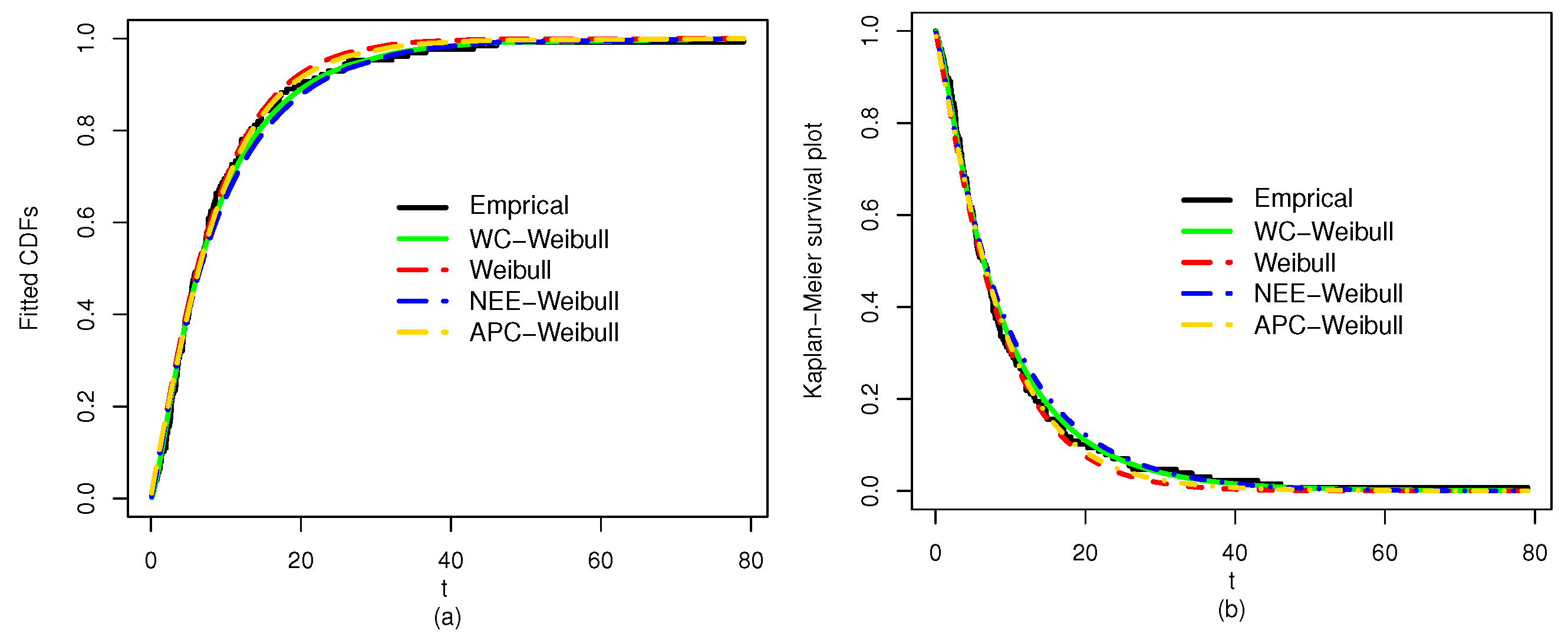
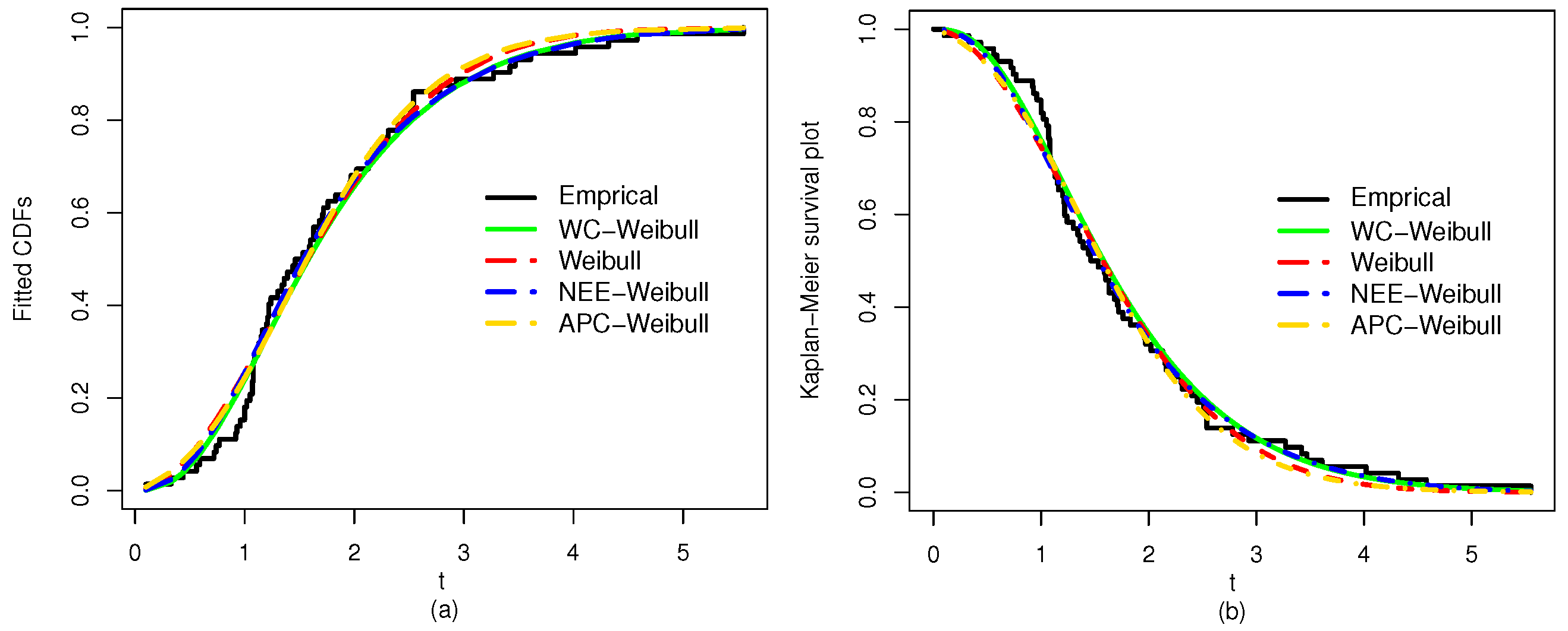
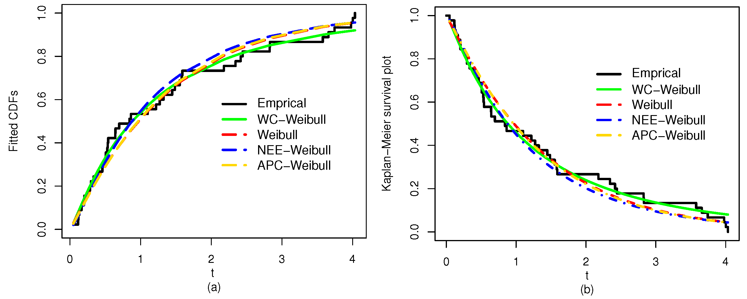
Figure 10.
The plots for the (a) fitted CDF and (b) fitted SF of the WC-Weibull and rival models for Data 1.
Figure 10.
The plots for the (a) fitted CDF and (b) fitted SF of the WC-Weibull and rival models for Data 1.
Figure 11.
The plots for the (a) log-likelihood profile of and (b) log-likelihood profile of of the WC-Weibull distribution for Data 2.
Figure 11.
The plots for the (a) log-likelihood profile of and (b) log-likelihood profile of of the WC-Weibull distribution for Data 2.
Figure 12.
The plots for the fitted PDF of (a) WC-Weibull distribution, (b) Weibull distribution, (c) NEE-Weibull distribution, and (d) NAC-Weibull distribution for Data 2.
Figure 12.
The plots for the fitted PDF of (a) WC-Weibull distribution, (b) Weibull distribution, (c) NEE-Weibull distribution, and (d) NAC-Weibull distribution for Data 2.
Figure 13.
The plots for the (a) fitted CDF and (b) fitted SF of the WC-Weibull and rival models for Data 2.
Figure 13.
The plots for the (a) fitted CDF and (b) fitted SF of the WC-Weibull and rival models for Data 2.
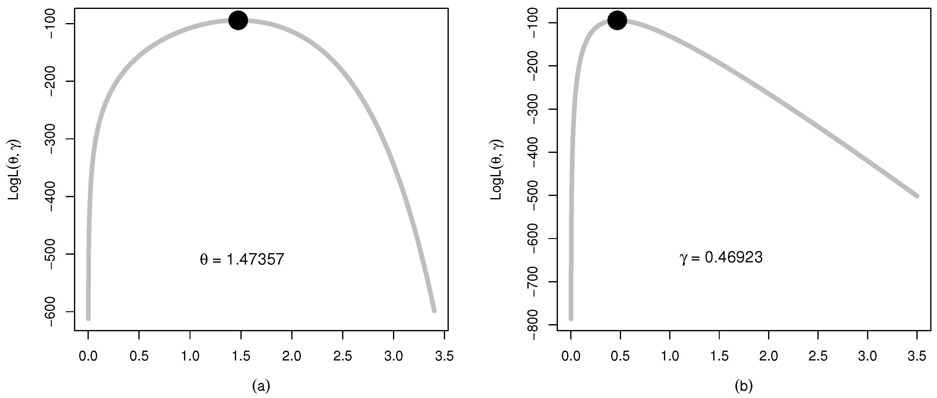
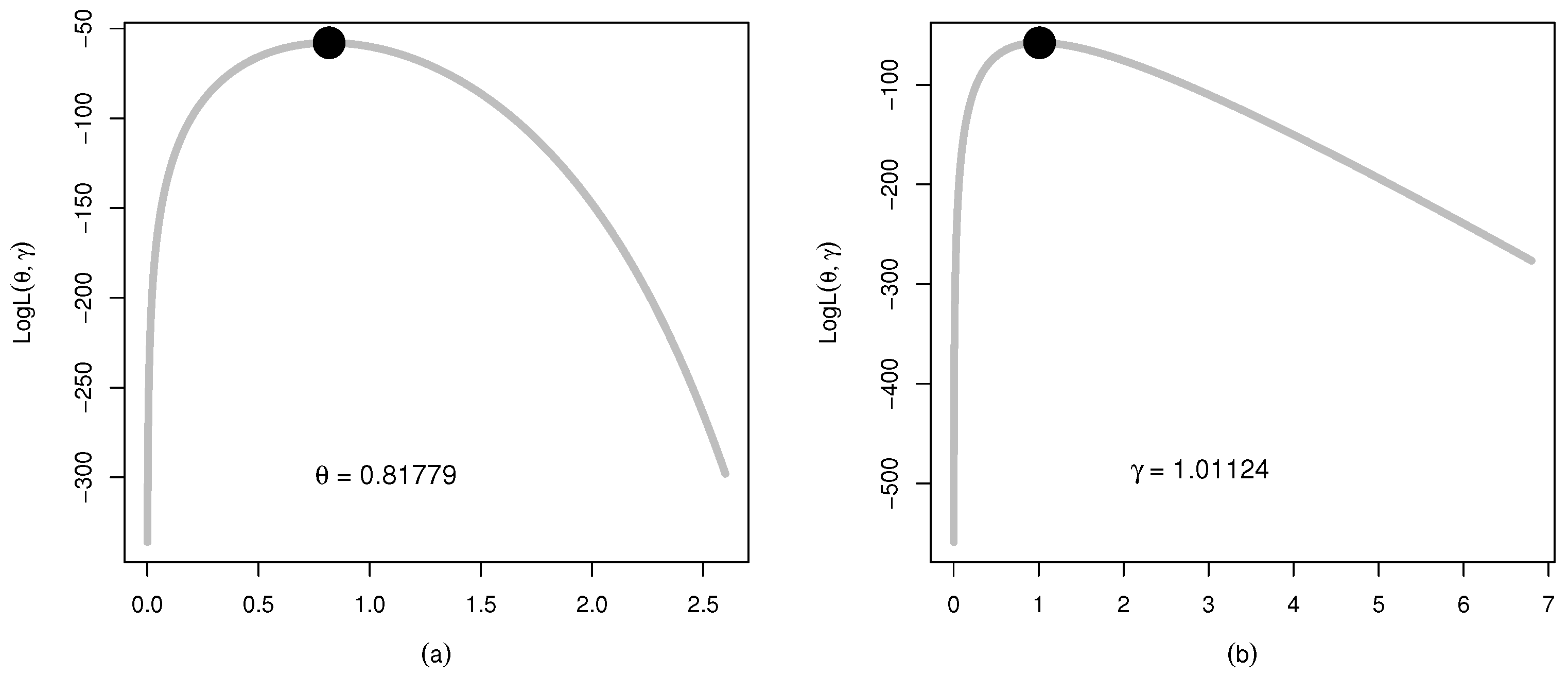
Figure 14.
The plots for the (a) log-likelihood profile of and (b) log-likelihood profile of of the WC-Weibull distribution for Data 3.
Figure 14.
The plots for the (a) log-likelihood profile of and (b) log-likelihood profile of of the WC-Weibull distribution for Data 3.
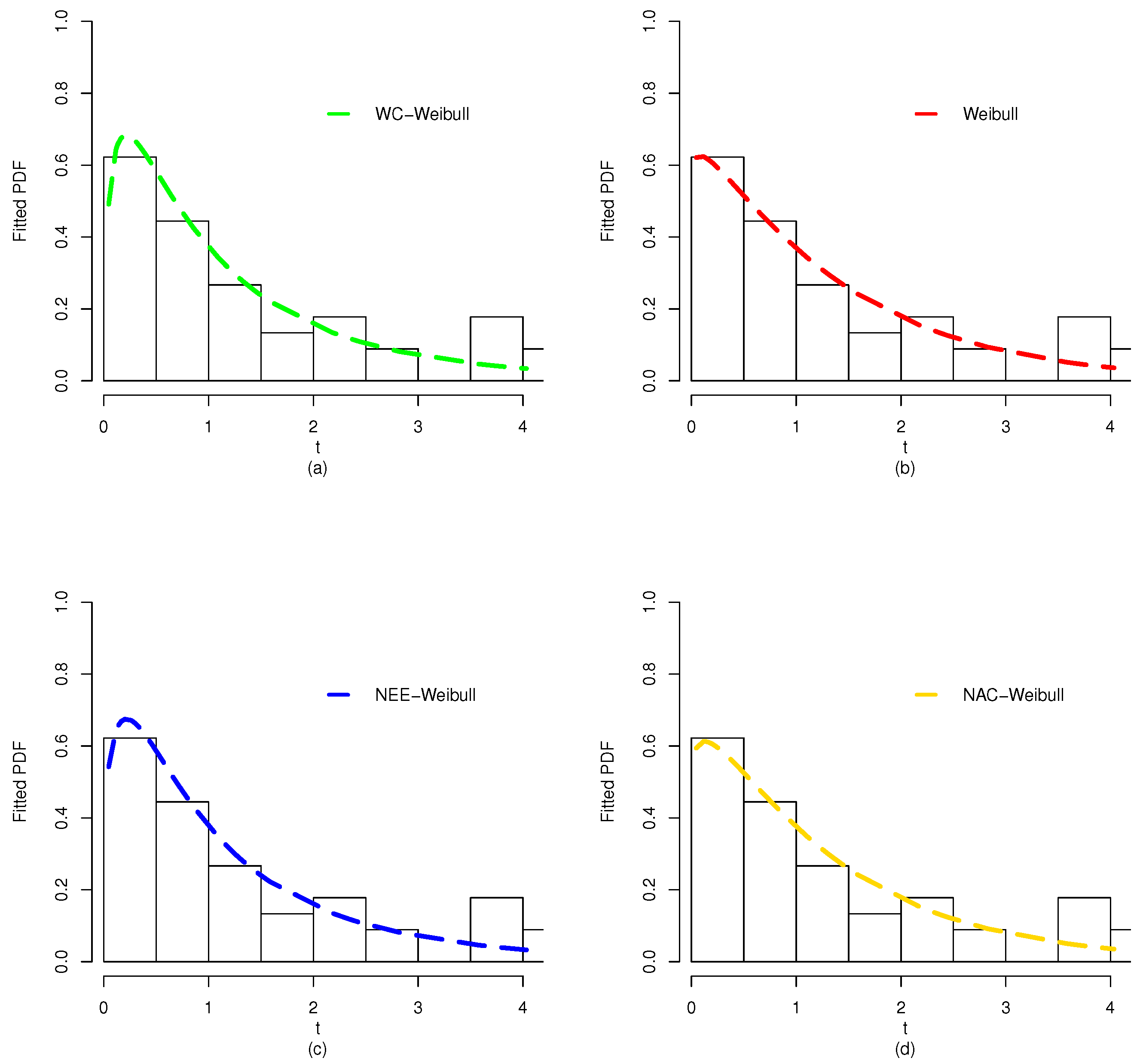
Figure 15.
The plots for the fitted PDF of (a) WC-Weibull distribution, (b) Weibull distribution, (c) NEE-Weibull distribution, and (d) NAC-Weibull distribution for Data 3.
Figure 15.
The plots for the fitted PDF of (a) WC-Weibull distribution, (b) Weibull distribution, (c) NEE-Weibull distribution, and (d) NAC-Weibull distribution for Data 3.
Figure 16.
The plots for the (a) fitted CDF and (b) fitted SF of the WC-Weibull and rival models for Data 3.
Figure 16.
The plots for the (a) fitted CDF and (b) fitted SF of the WC-Weibull and rival models for Data 3.
Table 1.
Numerical description of certain key measures of the WC-Weibull distribution.
Table 1.
Numerical description of certain key measures of the WC-Weibull distribution.
| Parameters | Measures |
|---|
| | | | | | | CV | Skewness | Kurtosis |
|---|
| 0.25 | 0.5 | 39.8608 | 7667.83 | | | 6078.95 | 1.956 | 36.9047 | 74.8206 |
| 1.0 | 4.82182 | 39.8608 | 480.029 | 7667.83 | 16.6109 | 0.845251 | 3.55452 | 8.51061 |
| 2.0 | 2.02246 | 4.82182 | 13.123 | 39.8608 | 0.731455 | 0.422876 | 0.434448 | 3.44383 |
| 3.0 | 1.56719 | 2.65779 | 4.82182 | 9.27623 | 0.201703 | 0.286572 | 0.0722435 | 2.92154 |
| 0.7 | 0.5 | 5.08429 | 124.75 | 7614.9 | 869357. | 98.9 | 1.956 | 36.9047 | 74.8206 |
| 1.0 | 1.72208 | 5.08429 | 21.8672 | 124.75 | 2.11874 | 0.845251 | 3.55452 | 8.51061 |
| 2.0 | 1.20865 | 1.72208 | 2.80088 | 5.08429 | 0.261234 | 0.422876 | 0.434448 | 3.44383 |
| 3.0 | 1.11191 | 1.33787 | 1.72208 | 2.3505 | 0.101533 | 0.286572 | 0.0722435 | 2.92154 |
| 2.0 | 0.5 | 0.622826 | 1.87203 | 13.9982 | 195.768 | 1.48412 | 1.956 | 36.9047 | 74.8206 |
| 1.0 | 0.602727 | 0.622826 | 0.937557 | 1.87203 | 0.259545 | 0.845251 | 3.55452 | 8.51061 |
| 2.0 | 0.715049 | 0.602727 | 0.579959 | 0.622826 | 0.0914319 | 0.422876 | 0.434448 | 3.44383 |
| 3.0 | 0.783595 | 0.664447 | 0.602727 | 0.579765 | 0.0504257 | 0.286572 | 0.0722435 | 2.92154 |
| 3.0 | 0.5 | 0.276811 | 0.369784 | 1.22892 | 7.63857 | 0.293159 | 1.956 | 36.9047 | 74.8206 |
| 1.0 | 0.401818 | 0.276811 | 0.277795 | 0.369784 | 0.115354 | 0.845251 | 3.55452 | 8.51061 |
| 2.0 | 0.583835 | 0.401818 | 0.31569 | 0.276811 | 0.0609546 | 0.422876 | 0.434448 | 3.44383 |
| 3.0 | 0.684533 | 0.507068 | 0.401818 | 0.337647 | 0.038482 | 0.286572 | 0.0722435 | 2.92154 |
Table 2.
The simulation results (numerical illustration) of the WC-Weibull distribution for and .
Table 2.
The simulation results (numerical illustration) of the WC-Weibull distribution for and .
| w | Parameters | MLEs | MSEs | Biases |
|---|
| 50 | | 1.4296460 | 0.02405948 | 0.02964635 |
| | | 1.0431000 | 0.03529194 | 0.04309999 |
| 100 | | 1.4212070 | 0.01200113 | 0.02120715 |
| | | 1.0130417 | 0.01491238 | 0.01304166 |
| 200 | | 1.4111950 | 0.00610701 | 0.01119543 |
| | | 1.0108342 | 0.00682204 | 0.01083417 |
| 300 | | 1.4081410 | 0.00375586 | 0.00814085 |
| | | 1.0101036 | 0.00518498 | 0.01010361 |
| 400 | | 1.4051080 | 0.00297678 | 0.00510784 |
| | | 1.0051150 | 0.00348963 | 0.00511498 |
| 500 | | 1.4036400 | 0.00241264 | 0.00364035 |
| | | 1.0023226 | 0.00277201 | 0.00232259 |
| 600 | | 1.4024130 | 0.00192576 | 0.00241314 |
| | | 1.0052975 | 0.00220275 | 0.00529752 |
| 700 | | 1.4023780 | 0.00169136 | 0.00237846 |
| | | 0.9983985 | 0.00209227 | −0.00160147 |
| 800 | | 1.4015180 | 0.00132295 | 0.00151838 |
| | | 1.0030077 | 0.00186708 | 0.00300772 |
| 900 | | 1.4025340 | 0.00123326 | 0.00253402 |
| | | 1.0011655 | 0.00173252 | 0.00116550 |
| 1000 | | 1.4027230 | 0.00113616 | 0.00272319 |
| | | 0.9995966 | 0.00133558 | −0.00040337 |
Table 3.
The simulation results (numerical illustration) of the WC-Weibull distribution for and .
Table 3.
The simulation results (numerical illustration) of the WC-Weibull distribution for and .
| w | Parameters | MLEs | MSEs | Biases |
|---|
| 50 | | 0.9301292 | 0.010420608 | 0.030129186 |
| | | 1.2587990 | 0.054114017 | 0.058799380 |
| 100 | | 0.9190032 | 0.004904806 | 0.019003196 |
| | | 1.2302100 | 0.023946464 | 0.030209555 |
| 200 | | 0.9083318 | 0.002087803 | 0.008331841 |
| | | 1.2147470 | 0.009057488 | 0.014747452 |
| 300 | | 0.9067783 | 0.001287310 | 0.006778291 |
| | | 1.2107980 | 0.006254901 | 0.010797619 |
| 400 | | 0.9048156 | 0.000789564 | 0.004815557 |
| | | 1.2079350 | 0.003876875 | 0.007935161 |
| 500 | | 0.9015265 | 0.000492410 | 0.001526458 |
| | | 1.2020270 | 0.002638221 | 0.002026584 |
| 600 | | 0.9035450 | 0.000448842 | 0.003544961 |
| | | 1.2037500 | 0.001965831 | 0.003750256 |
| 700 | | 0.9027654 | 0.000369818 | 0.002765412 |
| | | 1.2025920 | 0.001510795 | 0.002592192 |
| 800 | | 0.9020800 | 0.000248739 | 0.002080045 |
| | | 1.2008570 | 0.001217765 | 0.000856731 |
| 900 | | 0.9017151 | 0.000199939 | 0.001715065 |
| | | 1.2028740 | 0.001146012 | 0.002873864 |
| 1000 | | 0.9026201 | 0.000202154 | 0.002620059 |
| | | 1.2004670 | 0.000825658 | 0.000466553 |
Table 4.
The simulation results (numerical illustration) of the WC-Weibull distribution for and .
Table 4.
The simulation results (numerical illustration) of the WC-Weibull distribution for and .
| w | Parameters | MLEs | MSEs | Biases |
|---|
| 50 | | 1.1307770 | 0.017107187 | 0.030776790 |
| | | 0.8234098 | 0.019228798 | 0.002340984 |
| 100 | | 1.1162240 | 0.007458450 | 0.016223649 |
| | | 0.8115002 | 0.009817093 | 0.001150019 |
| 200 | | 1.1089390 | 0.003489588 | 0.008939034 |
| | | 0.8071731 | 0.004698275 | 0.000717306 |
| 300 | | 1.1080430 | 0.002455605 | 0.008043088 |
| | | 0.8028852 | 0.002875517 | 0.000288516 |
| 400 | | 1.1057100 | 0.001785741 | 0.005709626 |
| | | 0.8017098 | 0.002251494 | 0.000170975 |
| 500 | | 1.1046660 | 0.001251863 | 0.004666320 |
| | | 0.8029802 | 0.001741128 | 0.000298020 |
| 600 | | 1.1028690 | 0.001034179 | 0.002868828 |
| | | 0.8000814 | 0.001298472 | 0.000008142 |
| 700 | | 1.1026830 | 0.000934220 | 0.002683266 |
| | | 0.8024500 | 0.001270398 | 0.000245001 |
| 800 | | 1.1021630 | 0.000702283 | 0.002163235 |
| | | 0.8003387 | 0.001051193 | 0.000033872 |
| 900 | | 1.1028780 | 0.000730588 | 0.002878359 |
| | | 0.8012919 | 0.000900604 | 0.000129185 |
| 1000 | | 1.1021200 | 0.000572035 | 0.002120053 |
| | | 0.8009227 | 0.000773674 | 0.000009226 |
Table 5.
The numerical values of and along with standard errors (presented in the parenthesis) of the fitted models for Data 1.
Table 5.
The numerical values of and along with standard errors (presented in the parenthesis) of the fitted models for Data 1.
| Dist. | | | | |
|---|
| WC-Weibull | 0.85133 (0.05379) | 0.18984 (0.02808) | - | - |
| Weibull | 1.05357 (0.06668) | 0.09165 (0.01832) | - | - |
| NEE-Weibull | 1.20118 (0.20839) | 0.04084 (0.02911) | 0.92755 (0.52344) | - |
| NAC-Weibull | 0.75268 (0.10561) | 0.17150 (0.07296) | - | 8.00968 (8.67012) |
Table 6.
The values of the decisive tools of the WC-Weibull and its rival probability distributions for Data 1.
Table 6.
The values of the decisive tools of the WC-Weibull and its rival probability distributions for Data 1.
| Dist. | CM | AD | KS | p-Value | AIC | CAIC | BIC | HQIC |
|---|
| WC-Weibull | 0.0568 | 0.3645 | 0.0497 | 0.9089 | 826.3411 | 826.4371 | 832.0452 | 828.6587 |
| Weibull | 0.1324 | 0.7925 | 0.0742 | 0.4798 | 832.1903 | 832.2863 | 837.8943 | 834.5078 |
| NEE-Weibull | 0.0816 | 0.5073 | 0.0625 | 0.6993 | 831.1741 | 831.3676 | 837.7302 | 834.3505 |
| NAC-Weibull | 0.1248 | 0.7378 | 0.0667 | 0.6185 | 833.1293 | 833.3229 | 841.6854 | 836.6057 |
Table 7.
The numerical values of and along with standard errors (presented in the parenthesis) of the fitted models for Data 2.
Table 7.
The numerical values of and along with standard errors (presented in the parenthesis) of the fitted models for Data 2.
| Dist. | | | | |
|---|
| WC-Weibull | 1.47357 (0.12474) | 0.46923 (0.06400) | - | - |
| Weibull | 1.82376 (0.15865) | 0.28374 (0.054179) | - | - |
| NEE-Weibull | 2.34318 (0.61212) | 0.07853 (0.11671) | 0.31447 (0.55515) | - |
| NAC-Weibull | 1.22748 (0.20337) | 0.45063 (0.14358) | - | 13.81467 (15.71335) |
Table 8.
The values of the decisive tools of the WC-Weibull and its rival probability distributions for Data 2.
Table 8.
The values of the decisive tools of the WC-Weibull and its rival probability distributions for Data 2.
| Dist. | CM | AD | KS | p-Value | AIC | CAIC | BIC | HQIC |
|---|
| WC-Weibull | 0.1008 | 0.6203 | 0.0931 | 0.5602 | 192.5671 | 192.7410 | 197.1205 | 194.3798 |
| Weibull | 0.1647 | 0.9702 | 0.1051 | 0.4032 | 195.5797 | 195.7536 | 200.1331 | 197.3924 |
| NEE-Weibull | 0.1191 | 0.6590 | 0.1069 | 0.3821 | 194.5930 | 194.9460 | 200.4230 | 196.3121 |
| NAC-Weibull | 0.1565 | 0.9033 | 0.1018 | 0.4444 | 196.4686 | 196.8215 | 203.2986 | 199.1876 |
Table 9.
The numerical values of and along with standard errors (presented in the parenthesis) of the fitted models for Data 3.
Table 9.
The numerical values of and along with standard errors (presented in the parenthesis) of the fitted models for Data 3.
| Dist. | | | | |
|---|
| WC-Weibull | 0.81779 (0.08997) | 1.01124 (0.13157) | - | - |
| Weibull | 1.05460 (0.15865) | 0.71613 (0.05417) | - | - |
| NEE-Weibull | 1.26571 (0.20517) | 0.38501 (0.21702) | 0.62759 (0.73089) | - |
| NAC-Weibull | 1.08096 (0.20755) | 0.33115 (0.19496) | - | 0.49814 (0.89409) |
Table 10.
The values of the decisive tools of the WC-Weibull and its rival probability distributions for Data 3.
Table 10.
The values of the decisive tools of the WC-Weibull and its rival probability distributions for Data 3.
| Dist. | CM | AD | KS | p-Value | AIC | CAIC | BIC | HQIC |
|---|
| WC-Weibull | 0.0618 | 0.4282 | 0.0936 | 0.7909 | 119.7899 | 120.0756 | 123.4032 | 121.1369 |
| Weibull | 0.0813 | 0.5439 | 0.1102 | 0.6055 | 122.2476 | 122.5334 | 125.8610 | 123.5947 |
| NEE-Weibull | 0.0661 | 0.4523 | 0.0986 | 0.7215 | 121.6609 | 122.2462 | 127.0808 | 123.6814 |
| NAC-Weibull | 0.0803 | 0.5377 | 0.1115 | 0.5913 | 122.2846 | 122.8700 | 127.7046 | 124.3052 |


