
Enhancing Dynamic Parameter Adaptation in the Bird Swarm Algorithm Using General Type-2 Fuzzy Analysis and Mathematical Functions


Abstract
:1. Introduction
2. Basic Concepts
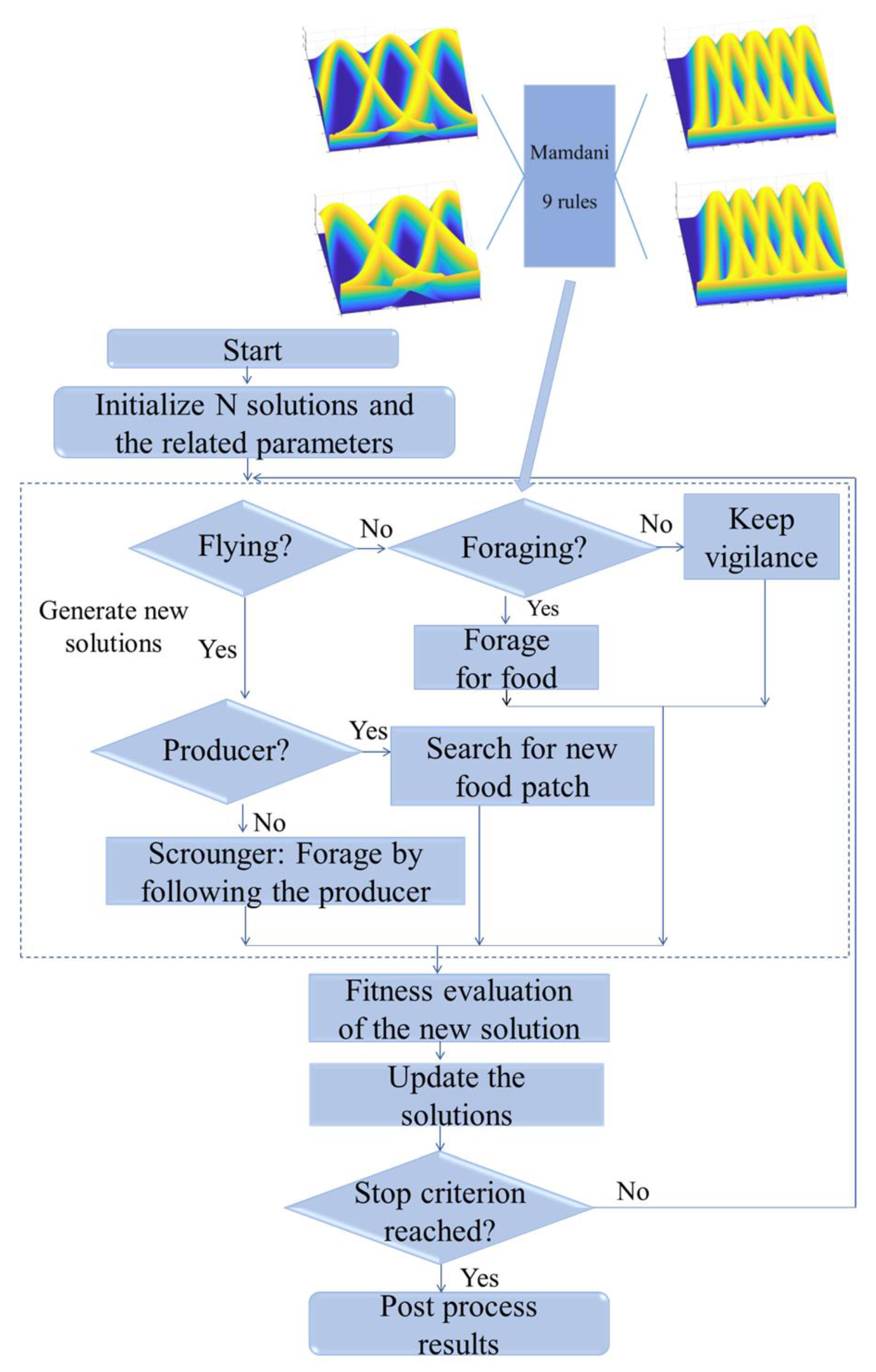
2.1. Bird Swarm Algorithm
| Algorithm 1: Bird Swarm Algorithm, BSA Pseudocode [28] |
| 1: Input N: the number of individuals (birds) contained by the population |
| 2: M: the maximum number of iterations |
| 3: FQ: the frequency of birds’ flight behaviors |
| 4: P: the probability of foraging for food |
| 5: C, S, a1, a2, FL: five constant parameters |
| 6: t=0; Initialize the population and define the related parameters |
| 7: Evaluate the N individuals’ fitness value, and find the best solution |
| 8: While (t < M) |
| 9: If (t % FQ ≠ 0) |
| 10: For i = 1 : N |
| 11: If rand (0,1) < P |
| 12: Birds forage for food (Equation (1)) |
| 13: Else |
| 14: Birds keep vigilance (Equation (2)) |
| 15: End if |
| 16: End for |
| 17: Else |
| 18: Divide the swarm into two parts: producers and scroungers. |
| 19: For i = 1 : N |
| 20: If i is a producer |
| 21: Producing (Equation (5)) |
| 22: Else |
| 23: Scrounging (Equation (6)) |
| 24: End if End For |
| 25: End If Evaluate new solutions |
| 26: if the new solutions are better than their previous ones, update then |
| 27: Find the best solutions |
| 28: t=t+1; End while |
| 29: Output: the individual with the best objective function value in the |
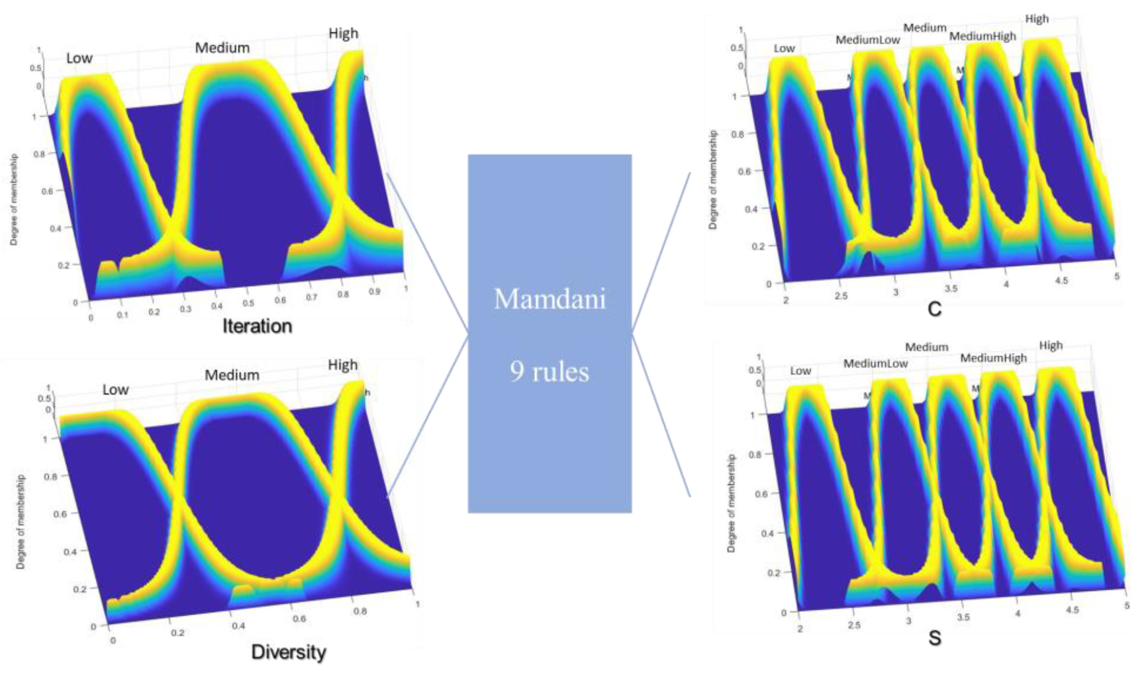
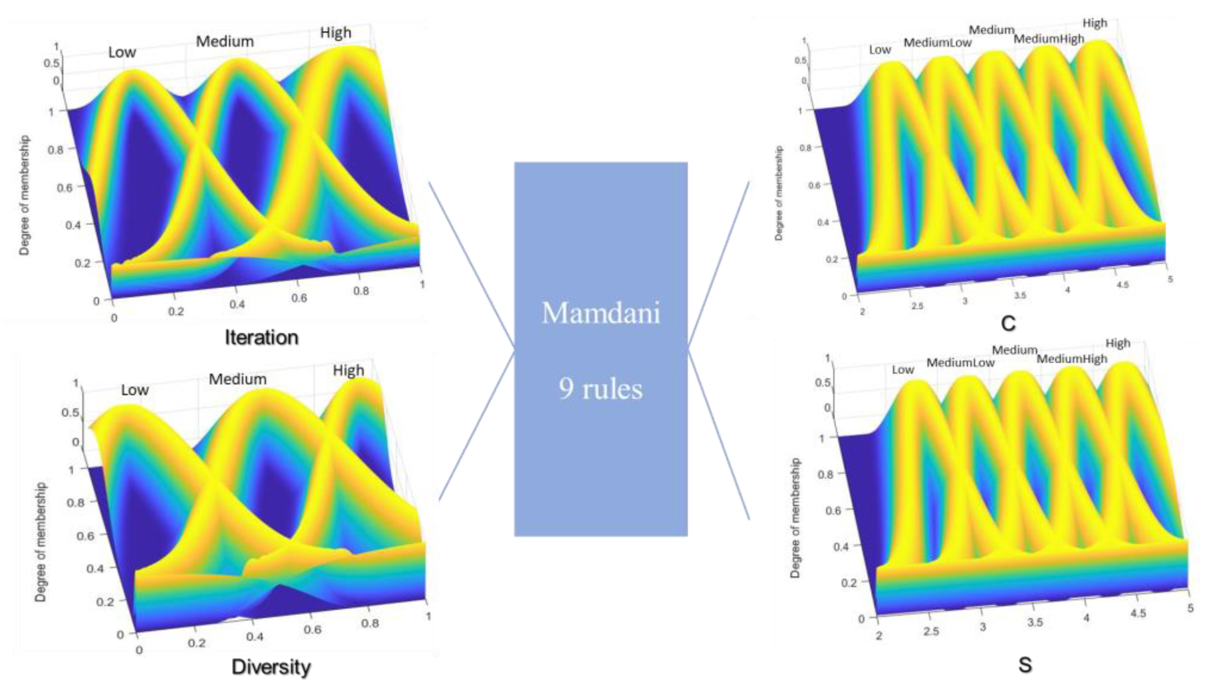
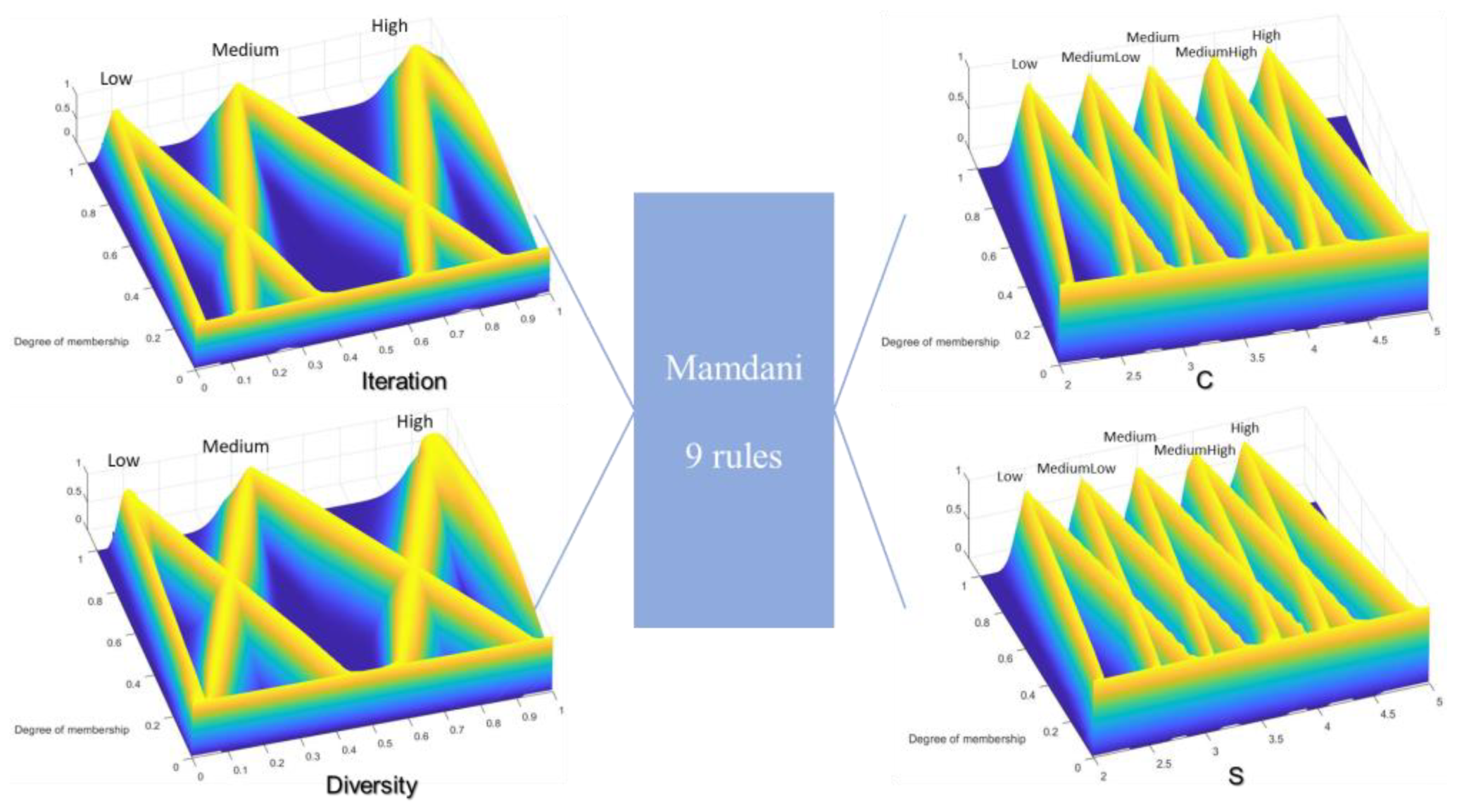
2.2. General Type-2 Fuzzy System
3. Problem Statement and Proposed Method
4. Results and Discussion
4.1. First Study Case
4.2. Second Study Case
4.3. Statistical Test
4.3.1. Statistical Test for the CEC2017 Functions
4.3.2. Statistical Test for the CEC2019 Functions
4.3.3. ANOVA Test for the Comparison of Bio-Inspired Optimization Methods
4.4. Discussion
5. Conclusions
Author Contributions
Funding
Data Availability Statement
Acknowledgments
Conflicts of Interest
References
- Jadhav, M.; Deshpande, V.; Midhunchakkaravarthy, D.; Waghole, D. Improving 5G Network Performance for OFDM-IDMA System Resource Management Optimization Using Bio-Inspired Algorithm with RSM. Comput. Commun. 2022, 193, 23–37. [Google Scholar] [CrossRef]
- Sarkar, T.; Salauddin, M.; Mukherjee, A.; Shariati, M.A.; Rebezov, M.; Tretyak, L.; Pateiro, M.; Lorenzo, J.M. Application of Bio-Inspired Optimization Algorithms in Food Processing. Curr. Res. Food Sci. 2022, 5, 432–450. [Google Scholar] [CrossRef] [PubMed]
- Raychaudhuri, A.; De, D. Bio-Inspired Algorithm for Multi-Objective Optimization in Wireless Sensor Network. In Nature Inspired Computing for Wireless Sensor Networks; Springer: Singapore, 2020; pp. 279–301. [Google Scholar]
- Gibson, S.; Issac, B.; Zhang, L.; Jacob, S.M. Detecting Spam Email with Machine Learning Optimized with Bio-Inspired Metaheuristic Algorithms. IEEE Access 2020, 8, 187914–187932. [Google Scholar] [CrossRef]
- Vijh, S.; Gaurav, P.; Pandey, H.M. Hybrid Bio-Inspired Algorithm and Convolutional Neural Network for Automatic Lung Tumor Detection. Neural Comput. Appl. 2020, 1–14. [Google Scholar] [CrossRef]
- Adam, S.P.; Alexandropoulos, S.-A.N.; Pardalos, P.M.; Vrahatis, M.N. No Free Lunch Theorem: A Review. In Approximation and Optimization: Algorithms, Complexity and Applications; Springer International Publishing: Cham, Switzerland, 2019; pp. 57–82. [Google Scholar]
- Jiang, Y.; Wu, Q.; Zhu, S.; Zhang, L. Orca Predation Algorithm: A Novel Bio-Inspired Algorithm for Global Optimization Problems. Expert Syst. Appl. 2022, 188, 116026. [Google Scholar] [CrossRef]
- Yuan, Y.; Ren, J.; Wang, S.; Wang, Z.; Mu, X.; Zhao, W. Alpine Skiing Optimization: A New Bio-Inspired Optimization Algorithm. Adv. Eng. Softw. 2022, 170, 103158. [Google Scholar] [CrossRef]
- Moldovan, D. Horse Optimization Algorithm: A Novel Bio-Inspired Algorithm for Solving Global Optimization Problems. In Artificial Intelligence and Bioinspired Computational Methods: Proceedings of the 9th Computer Science On-Line Conference 2020; Springer International Publishing: Cham, Switzerland, 2020; pp. 195–209. [Google Scholar]
- Zamani, H.; Nadimi-Shahraki, M.H.; Gandomi, A.H. Starling Murmuration Optimizer: A Novel Bio-Inspired Algorithm for Global and Engineering Optimization. Comput. Methods Appl. Mech. Eng. 2022, 392, 114616. [Google Scholar] [CrossRef]
- Sulaiman, M.H.; Mustaffa, Z.; Saari, M.M.; Daniyal, H. Barnacles Mating Optimizer: A New Bio-Inspired Algorithm for Solving Engineering Optimization Problems. Eng. Appl. Artif. Intell. 2020, 87, 103330. [Google Scholar] [CrossRef]
- Rangel-Carrillo, E.; Hernandez-Vargas, E.A.; Arana-Daniel, N.; Lopez-Franco, C.; Alanis, A.Y. Particle Swarm Optimization Algorithm with a Bio-Inspired Aging Model. In Particle Swarm Optimization with Applications; Erdoğmuş, P., Ed.; IntechOpen: Rijeka, Croatia, 2017; Chapter 2. [Google Scholar]
- Yang, X.-S. Genetic Algorithms. In Nature-Inspired Optimization Algorithms; Academic Press: London, UK, 2021; pp. 91–100. [Google Scholar]
- Dhiman, G. ESA: A Hybrid Bio-Inspired Metaheuristic Optimization Approach for Engineering Problems. Eng. Comput. 2021, 37, 323–353. [Google Scholar] [CrossRef]
- Moin, M.M.; Narayan, D.G.; Patil, S. A Hybrid Bio-Inspired Algorithm for Routing in Software Defined Networks. In Proceedings of the 2021 12th International Conference on Computing Communication and Networking Technologies (ICCCNT), Kharagpur, India, 6–8 July 2021; pp. 1–7. [Google Scholar]
- Vijh, S.; Saraswat, M.; Kumar, S. Automatic Multilevel Image Thresholding Segmentation Using Hybrid Bio-Inspired Algorithm and Artificial Neural Network for Histopathology Images. Multimedia Tools Appl. 2023, 82, 4979–5010. [Google Scholar] [CrossRef]
- Sun, G.; Lan, Y.; Zhao, R. Differential Evolution with Gaussian Mutation and Dynamic Parameter Adjustment. Soft Comput. 2019, 23, 1615–1642. [Google Scholar] [CrossRef]
- Zhou, X.; Ma, H.; Gu, J.; Chen, H.; Deng, W. Parameter Adaptation-Based Ant Colony Optimization with Dynamic Hybrid Mechanism. Eng. Appl. Artif. Intell. 2022, 114, 105139. [Google Scholar] [CrossRef]
- Chen, X.; Huang, J. Towards Environmentally Adaptive Odor Source Localization: Fuzzy Lévy Taxis Algorithm and Its Validation in Dynamic Odor Plumes. In Proceedings of the 2020 5th International Conference on Advanced Robotics and Mechatronics (ICARM), Shenzhen, China, 18–21 December 2020; pp. 282–287. [Google Scholar]
- Castillo, O.; Aguilar, L.T. Background on Type-1 and Type-2 Fuzzy Logic. In Type-2 Fuzzy Logic in Control of Nonsmooth Systems: Theoretical Concepts and Applications; Springer International Publishing: Cham, Switzerland, 2019; pp. 5–19. [Google Scholar]
- Zadeh, L.A. Fuzzy Logic. In Granular, Fuzzy, and Soft Computing; Springer: New York, NY, USA, 2023; pp. 19–49. [Google Scholar]
- Janarthanan, R.; Balamurali, R.; Annapoorani, A.; Vimala, V. Prediction of Rainfall Using Fuzzy Logic. Mater. Today Proc. 2021, 37, 959–963. [Google Scholar] [CrossRef]
- Thakkar, H.; Shah, V.; Yagnik, H.; Shah, M. Comparative Anatomization of Data Mining and Fuzzy Logic Techniques Used in Diabetes Prognosis. Clin. eHealth 2021, 4, 12–23. [Google Scholar] [CrossRef]
- Robinson, F.A. Fuzzy Logic and Fuzzy Hybrid Techniques for Construction Engineering and Management. J. Constr. Eng. Manag. 2020, 146, 04020064. [Google Scholar]
- Serrano-Guerrero, J.; Romero, F.P.; Olivas, J.A. Fuzzy Logic Applied to Opinion Mining: A Review. Knowl. Based Syst. 2021, 222, 107018. [Google Scholar] [CrossRef]
- Miramontes, I.; Melin, P. Interval Type-2 Fuzzy Approach for Dynamic Parameter Adaptation in the Bird Swarm Algorithm for the Optimization of Fuzzy Medical Classifier. Axioms 2022, 11, 485. [Google Scholar] [CrossRef]
- Melin, P.; Miramontes, I.; Carvajal, O.; Prado-Arechiga, G. Fuzzy Dynamic Parameter Adaptation in the Bird Swarm Algorithm for Neural Network Optimization. Soft Comput. 2022, 26, 9497–9514. [Google Scholar] [CrossRef]
- Meng, X.B.; Gao, X.Z.; Lu, L.; Liu, Y.; Zhang, H. A New Bio-Inspired Optimisation Algorithm: Bird Swarm Algorithm. J. Exp. Theor. Artif. Intell. 2016, 28, 673–687. [Google Scholar] [CrossRef]
- Xiang, L.; Deng, Z.; Hu, A. Forecasting Short-Term Wind Speed Based on IEWT-LSSVM Model Optimized by Bird Swarm Algorithm. IEEE Access 2019, 7, 59333–59345. [Google Scholar] [CrossRef]
- Varol Altay, E.; Alatas, B. Bird Swarm Algorithms with Chaotic Mapping. Artif. Intell. Rev. 2020, 53, 1373–1414. [Google Scholar] [CrossRef]
- Ahmad, M.; Javaid, N.; Niaz, I.A.; Shafiq, S.; Rehman, O.U.; Hussain, H.M. Application of Bird Swarm Algorithm for Solution of Optimal Power Flow Problems. Proc. Adv. Intell. Syst. Comput. 2019, 772, 280–291. [Google Scholar]
- Huang, C.; Sheng, X. Data-Driven Model Identification of Boiler-Turbine Coupled Process in 1000 MW Ultra-Supercritical Unit by Improved Bird Swarm Algorithm. Energy 2020, 205, 118009. [Google Scholar] [CrossRef]
- Zhang, C.; Yu, S.; Li, G.; Xu, Y. The Recognition Method of MQAM Signals Based on BP Neural Network and Bird Swarm Algorithm. IEEE Access 2021, 9, 36078–36086. [Google Scholar] [CrossRef]
- Gonzalez, C.I.; Melin, P.; Castro, J.R.; Castillo, O. Generalized Type-2 Fuzzy Logic. In Edge Detection Methods Based on Generalized Type-2 Fuzzy Logic; Springer International Publishing: Cham, Switzerland, 2017; pp. 3–9. [Google Scholar]
- Ontiveros, E.; Melin, P.; Castillo, O. Comparative Study of Interval Type-2 and General Type-2 Fuzzy Systems in Medical Diagnosis. Inf. Sci. 2020, 525, 37–53. [Google Scholar] [CrossRef]
- Mendel, J.M. General Type-2 Fuzzy Logic Systems Made Simple: A Tutorial. IEEE Trans. Fuzzy Syst. 2014, 22, 1162–1182. [Google Scholar] [CrossRef]
- Castro, J.R.; Sanchez, M.A.; Gonzalez, C.I.; Melin, P.; Castillo, O. A New Method for Parameterization of General Type-2 Fuzzy Sets. Fuzzy Inf. Eng. 2018, 10, 31–57. [Google Scholar] [CrossRef]
- Mendel, J.M. Type-2 Fuzzy Sets as Well as Computing with Words. IEEE Comput. Intell. Mag. 2019, 14, 82–95. [Google Scholar] [CrossRef]
- Gonzalez, C.I.; Melin, P.; Castillo, O. Edge Detection Method Based on General Type-2 Fuzzy Logic Applied to Color Images. Information 2017, 8, 104. [Google Scholar] [CrossRef]
- Olivas, F.; Valdez, F.; Castillo, O.; Melin, P. Dynamic Parameter Adaptation in Particle Swarm Optimization Using Interval Type-2 Fuzzy Logic. Soft Comput. 2016, 20, 1057–1070. [Google Scholar] [CrossRef]
- Bouzbita, S.; El Afia, A.; Faizi, R. The Behaviour of ACS-TSP Algorithm When Adapting Both Pheromone Parameters Using Fuzzy Logic Controller. Int. J. Electr. Comput. Eng. 2020, 10, 5436–5444. [Google Scholar] [CrossRef]
- Kumar Sahoo, S.; Houssein, E.H.; Premkumar, M.; Kumar Saha, A.; Emam, M.M. Self-Adaptive Moth Flame Optimizer Combined with Crossover Operator and Fibonacci Search Strategy for COVID-19 CT Image Segmentation. Expert Syst. Appl. 2023, 227, 120367. [Google Scholar] [CrossRef] [PubMed]
- Chen, H.; Zhang, Q.; Luo, J.; Xu, Y.; Zhang, X. An Enhanced Bacterial Foraging Optimization and Its Application for Training Kernel Extreme Learning Machine. Appl. Soft Comput. J. 2020, 86, 105884. [Google Scholar] [CrossRef]
- Rahman, C.M.; Rashid, T.A. Dragonfly Algorithm and Its Applications in Applied Science Survey. Comput. Intell. Neurosci. 2019, 2019, 9293617. [Google Scholar] [CrossRef] [PubMed]
- Ahmed, A.M.; Rashid, T.A.; Saeed, S.A.M. Cat Swarm Optimization Algorithm: A Survey and Performance Evaluation. Comput. Intell. Neurosci. 2020, 2020, 4854895. [Google Scholar] [CrossRef] [PubMed]


| Rule | Antecedent | Consequent | ||
|---|---|---|---|---|
| Iteration | Diversity | C | S | |
| 1 | Low | Low | High | Low |
| 2 | Low | Medium | Medium High | Medium |
| 3 | Low | High | Medium High | Medium Low |
| 4 | Medium | Low | Medium High | Medium Low |
| 5 | Medium | Medium | Medium | Medium |
| 6 | Medium | High | Medium Low | Medium High |
| 7 | High | Low | Medium | High |
| 8 | High | Medium | Medium Low | Medium High |
| 9 | High | High | Low | High |
| Rule | Antecedent | Consequent | ||
|---|---|---|---|---|
| Iteration | Diversity | C | S | |
| 1 | Low | Low | Low | High |
| 2 | Low | Medium | Medium | Medium High |
| 3 | Low | High | Medium Low | Medium High |
| 4 | Medium | Low | Medium Low | Medium High |
| 5 | Medium | Medium | Medium | Medium |
| 6 | Medium | High | Medium High | Medium Low |
| 7 | High | Low | Medium | High |
| 8 | High | Medium | Medium High | Medium Low |
| 9 | High | High | High | Low |
| Rule | Antecedent | Consequent | ||
|---|---|---|---|---|
| Iteration | Diversity | C | S | |
| 1 | Low | Low | Low | High |
| 2 | Low | Medium | Low | Medium |
| 3 | Low | High | Medium | Medium Low |
| 4 | Medium | Low | Medium Low | Medium Low |
| 5 | Medium | Medium | Medium | Medium |
| 6 | Medium | High | Medium | Medium High |
| 7 | High | Low | Medium | High |
| 8 | High | Medium | Medium High | Medium High |
| 9 | High | High | High | High |
| Rule | Antecedent | Consequent | ||
|---|---|---|---|---|
| Iteration | Diversity | C | S | |
| 1 | Low | Low | High | High |
| 2 | Low | Medium | High | Medium |
| 3 | Low | High | Medium | Medium High |
| 4 | Medium | Low | High | Medium High |
| 5 | Medium | Medium | Medium | Medium |
| 6 | Medium | High | Medium | Medium Low |
| 7 | High | Low | Medium Low | Medium |
| 8 | High | Medium | Medium | Medium Low |
| 9 | High | High | Low | Low |
| Iteration | Population | Dim | FQ | a1 | a2 | C | S | |
|---|---|---|---|---|---|---|---|---|
| BSA | 1000 | 40 | 30 | 3 | 1 | 1 | 1.5 | 1.5 |
| GBSA | 1000 | 40 | 30 | 3 | 1 | 1 | Dynamic | Dynamic |
| Function | No. | Name Function | Fi |
|---|---|---|---|
| Unimodal Functions | 1 | Shifted and Rotated Bent Cigar | 100 |
| 2 | Shifted and Rotated Sum of Different Power | 200 | |
| 3 | Shifted and Rotated Zakharov | 300 | |
| Simple Multimodal Functions | 4 | Shifted and Rotated Rosenbrock | 400 |
| 5 | Shifted and Rotated Rastrigin’s | 500 | |
| 6 | Shifted and Rotated Expanded Scaffer’s F6 | 600 | |
| 7 | Shifted and Rotated Lunacek Bi-Rastrigin | 700 | |
| 8 | Shifted and Rotated Non-Continuous Rastrigin’s | 800 | |
| 9 | Shifted and Rotated Levy | 900 | |
| 10 | Shifted and Rotated Schwefel’s | 1000 | |
| Hybrid Functions | 11 | Hybrid Function 1 (N = 3) | 1100 |
| 12 | Hybrid Function 2 (N = 3) | 1200 | |
| 13 | Hybrid Function 3 (N = 3) | 1300 | |
| 14 | Hybrid Function 4 (N = 4) | 1400 | |
| 15 | Hybrid Function 5 (N = 4) | 1500 | |
| 16 | Hybrid Function 6 (N = 4) | 1600 | |
| 17 | Hybrid Function 6 (N = 5) | 1700 | |
| 18 | Hybrid Function 6 (N = 5) | 1800 | |
| 19 | Hybrid Function 6 (N = 5) | 1900 | |
| 20 | Hybrid Function 6 (N = 6) | 2000 | |
| Composition Functions | 21 | Composition Function 1 (N = 3) | 2100 |
| 22 | Composition Function 2 (N = 3) | 2200 | |
| 23 | Composition Function 3 (N = 4) | 2300 | |
| 24 | Composition Function 4 (N = 4) | 2400 | |
| 25 | Composition Function 5 (N = 5) | 2500 | |
| 26 | Composition Function 6 (N = 5) | 2600 | |
| 27 | Composition Function 7 (N = 6) | 2700 | |
| 28 | Composition Function 8 (N = 6) | 2800 | |
| 29 | Composition Function 9 (N = 3) | 2900 | |
| 30 | Composition Function 10 (N = 3) | 3000 |
| No. | Original | E×p3 | |
|---|---|---|---|
| 1 | Average | 3.180 × 10¹⁰ | 1.781 × 10⁹ |
| STD | 8.650 × 10⁹ | 8.623 × 10⁸ | |
| 2 | Average | 1.027 × 1046 | 5.981 × 1030 |
| STD | 7.631 × 1046 | 2.745 × 1031 | |
| 3 | Average | 7.630 × 10⁴ | 4.382 × 10⁴ |
| STD | 1.159 × 10⁴ | 8.945 × 10³ | |
| 4 | Average | 6.745 × 10³ | 7.782 × 10² |
| STD | 3.096 × 10³ | 1.336 × 10² | |
| 5 | Average | 8.488 × 10² | 7.365 × 10² |
| STD | 4.287 × 101 | 4.007 × 101 | |
| 6 | Average | 6.754 × 10² | 6.472 × 10² |
| STD | 8.922 × 10+ | 1.155 × 101 | |
| 7 | Average | 1.356 × 10³ | 1.083 × 10³ |
| STD | 8.106 × 101 | 6.379 × 101 | |
| 8 | Average | 1.088 × 10³ | 9.958 × 10² |
| STD | 3.624 × 101 | 2.760 × 101 | |
| 9 | Average | 7.636 × 10³ | 4.369 × 10³ |
| STD | 1.432 × 10³ | 1.482 × 10³ | |
| 10 | Average | 7.434 × 10³ | 7.146 × 10³ |
| STD | 6.253 × 10² | 8.492 × 10² | |
| 11 | Average | 5.847 × 10³ | 1.628 × 10³ |
| STD | 2.296 × 10³ | 1.689 × 10² | |
| 12 | Average | 2.988 × 10⁹ | 9.269 × 10⁷ |
| STD | 2.085 × 10⁹ | 7.411 × 10⁷ | |
| 13 | Average | 5.683 × 10⁸ | 2.794 × 10⁶ |
| STD | 1.437 × 10⁹ | 1.658 × 10⁷ | |
| 14 | Average | 2.576 × 10⁵ | 4.109 × 10⁴ |
| STD | 5.443 × 10⁵ | 1.714 × 10⁵ | |
| 15 | Average | 1.592 × 10⁷ | 4.673 × 10⁴ |
| STD | 4.983 × 10⁷ | 3.576 × 10⁴ | |
| 16 | Average | 4.126 × 10³ | 3.251 × 10³ |
| STD | 6.388 × 10² | 4.145 × 10² | |
| 17 | Average | 2.918 × 10³ | 2.410 × 10³ |
| STD | 3.704 × 10² | 2.557 × 10² | |
| 18 | Average | 2.237 × 10⁶ | 7.948 × 10⁵ |
| STD | 4.123 × 10⁶ | 4.848 × 10⁶ | |
| 19 | Average | 3.017 × 10⁷ | 2.534 × 10⁶ |
| STD | 6.582 × 10⁷ | 1.313 × 10⁷ | |
| 20 | Average | 2.831 × 10³ | 2.544 × 10³ |
| STD | 2.266 × 10² | 1.794 × 10² | |
| 21 | Average | 2.649 × 10³ | 2.504 × 10³ |
| STD | 5.301 × 101 | 4.408 × 101 | |
| 22 | Average | 8.312 × 10³ | 4.059 × 10³ |
| STD | 1.123 × 10³ | 2.387 × 10³ | |
| 23 | Average | 3.352 × 10³ | 3.027 × 10³ |
| STD | 1.546 × 10² | 1.096 × 10² | |
| 24 | Average | 3.537 × 10³ | 3.256 × 10³ |
| STD | 1.540 × 10² | 1.492 × 10² | |
| 25 | Average | 4.205 × 10³ | 3.094 × 10³ |
| STD | 4.789 × 10² | 7.383 × 101 | |
| 26 | Average | 9.949 × 10³ | 6.481 × 10³ |
| STD | 9.100 × 10² | 1.370 × 10³ | |
| 27 | Average | 3.768 × 10³ | 3.486 × 10³ |
| STD | 2.755 × 10² | 1.971 × 10² | |
| 28 | Average | 5.354 × 10³ | 3.459 × 10³ |
| STD | 6.885 × 10² | 8.772 × 101 | |
| 29 | Average | 6.121 × 10³ | 4.749 × 10³ |
| STD | 9.945 × 10² | 5.622 × 10² | |
| 30 | Average | 7.522 × 10⁷ | 6.593 × 10⁶ |
| STD | 1.239 × 10⁸ | 9.192 × 10⁶ |
| No. | GaussGauss | TrianGauss | GbellGbell | |
|---|---|---|---|---|
| 1 | Average | 1.781 × 10⁹ | 1.778 × 10⁹ | 1.657 × 10⁹ |
| STD | 8.623 × 10⁸ | 8.214 × 10⁸ | 6.997 × 10⁸ | |
| 2 | Average | 5.981 × 1030 | 2.267 × 1031 | 1.487 × 1041 |
| STD | 2.745 × 1031 | 1.147 × 1032 | 1.487 × 1042 | |
| 3 | Average | 4.382 × 10⁴ | 4.202 × 10⁴ | 4.440 × 10⁴ |
| STD | 8.945 × 10³ | 9.658 × 10³ | 9.395 × 10³ | |
| 4 | Average | 7.782 × 10² | 7.943 × 10² | 7.759 × 10² |
| STD | 1.336 × 10² | 1.329 × 10² | 1.894 × 10² | |
| 5 | Average | 7.365 × 10² | 7.356 × 10² | 7.242 × 10² |
| STD | 4.007 × 10+1 | 3.820 × 101 | 3.934 × 101 | |
| 6 | Average | 6.472 × 10+2 | 6.501 × 10² | 6.477 × 10² |
| STD | 1.155 × 10+1 | 1.108 × 101 | 1.028 × 101 | |
| 7 | Average | 1.083 × 10+3 | 1.089 × 10³ | 1.073 × 10³ |
| STD | 6.379 × 10+1 | 6.114 × 101 | 5.731 × 101 | |
| 8 | Average | 9.958 × 10+2 | 9.897 × 10² | 9.966 × 10² |
| STD | 2.760 × 10+1 | 2.908 × 101 | 2.844 × 101 | |
| 9 | Average | 4.369 × 10+3 | 4.581 × 10³ | 4.464 × 10³ |
| STD | 1.482 × 10³ | 1.330 × 10³ | 1.526 × 10³ | |
| 10 | Average | 7.146 × 10³ | 6.933 × 10³ | 6.936 × 10³ |
| STD | 8.492 × 10² | 7.594 × 10² | 8.918 × 10² | |
| 11 | Average | 1.628 × 10³ | 1.644 × 10³ | 1.635 × 10³ |
| STD | 1.689 × 10² | 1.794 × 10² | 1.657 × 10² | |
| 12 | Average | 9.269 × 10⁷ | 1.236 × 10⁸ | 1.166 × 10⁸ |
| STD | 7.411 × 10⁷ | 1.045 × 10⁸ | 9.353 × 10⁷ | |
| 13 | Average | 2.794 × 10⁶ | 9.930 × 10⁵ | 2.785 × 10⁷ |
| STD | 1.658 × 10⁷ | 1.831 × 10⁶ | 2.718 × 10⁸ | |
| 14 | Average | 4.109 × 10⁴ | 4.986 × 10⁴ | 3.721 × 10⁴ |
| STD | 1.714 × 10⁵ | 1.402 × 10⁵ | 1.131 × 10⁵ | |
| 15 | Average | 4.673 × 10⁴ | 4.731 × 10⁴ | 1.767 × 10⁷ |
| STD | 3.576 × 10⁴ | 4.330 × 10⁴ | 1.763 × 10⁸ | |
| 16 | Average | 3.251 × 10³ | 3.313 × 10³ | 3.225 × 10³ |
| STD | 4.145 × 10² | 4.546 × 10² | 3.943 × 10² | |
| 17 | Average | 2.410 × 10³ | 2.440 × 10³ | 2.422 × 10³ |
| STD | 2.557 × 10² | 2.868 × 10² | 2.333 × 10² | |
| 18 | Average | 7.948 × 10⁵ | 5.130 × 10⁵ | 4.112 × 10⁵ |
| STD | 4.848 × 10⁶ | 1.314 × 10⁶ | 5.422 × 10⁵ | |
| 19 | Average | 2.534 × 10⁶ | 4.943 × 10⁵ | 5.061 × 10⁵ |
| STD | 1.313 × 10⁷ | 7.708 × 10⁵ | 7.777 × 10⁵ | |
| 20 | Average | 2.544 × 10³ | 2.536 × 10³ | 2.561 × 10³ |
| STD | 1.794 × 10² | 1.697 × 10² | 1.899 × 10² | |
| 21 | Average | 2.504 × 10³ | 2.521 × 10³ | 2.511 × 10³ |
| STD | 4.408 × 101 | 4.128 × 101 | 3.535 × 101 | |
| 22 | Average | 4.059 × 10³ | 3.759 × 10³ | 4.207 × 10³ |
| STD | 2.387 × 10³ | 1.970 × 10³ | 2.333 × 10³ | |
| 23 | Average | 3.027 × 10³ | 3.023 × 10³ | 3.040 × 10³ |
| STD | 1.096 × 10² | 1.226 × 10² | 1.192 × 10² | |
| 24 | Average | 3.256 × 10³ | 3.269 × 10³ | 3.236 × 10³ |
| STD | 1.492 × 10² | 1.664 × 10² | 1.607 × 10² | |
| 25 | Average | 3.094 × 10³ | 3.092 × 10³ | 3.087 × 10³ |
| STD | 7.383 × 101 | 6.931 × 101 | 6.474 × 101 | |
| 26 | Average | 6.481 × 10³ | 6.693 × 10³ | 6.632 × 10³ |
| STD | 1.370 × 10³ | 1.661 × 10³ | 1.478 × 10³ | |
| 27 | Average | 3.486 × 10³ | 3.474 × 10³ | 3.470 × 10³ |
| STD | 1.971 × 10² | 2.024 × 10² | 1.773 × 10² | |
| 28 | Average | 3.459 × 10³ | 3.465 × 10³ | 3.470 × 10³ |
| STD | 8.772 × 101 | 8.233 × 101 | 9.007 × 101 | |
| 29 | Average | 4.749 × 10³ | 4.743 × 10³ | 4.744 × 10³ |
| STD | 5.622 × 10² | 5.443 × 10² | 5.336 × 10² | |
| 30 | Average | 6.593 × 10⁶ | 6.566 × 10⁶ | 6.482 × 10⁶ |
| STD | 9.192 × 10⁶ | 6.232 × 10⁶ | 8.134 × 10⁶ |
| GBSA | ||||||
|---|---|---|---|---|---|---|
| No. | Es-MFO | CCGBFO | GaussGauss | TrianGauss | GbellGbell | |
| 1 | Average | 6.21 × 10¹⁰ | 6.244 × 10¹⁰ | 1.781 × 10⁹ | 1.778 × 10⁹ | 1.657 × 10⁹ |
| STD | 1.01 × 10¹⁰ | 5.453 × 10⁹ | 8.623 × 10⁸ | 8.214 × 10⁸ | 6.997 × 10⁸ | |
| 3 | Average | 1.25 × 10⁵ | 8.408 × 10⁴ | 4.382 × 10⁴ | 4.202 × 10⁴ | 4.440 × 10⁴ |
| STD | 3.07 × 10⁴ | 6.060 × 10³ | 8.945 × 10³ | 9.658 × 10³ | 9.395 × 10³ | |
| 4 | Average | 1.66 × 10⁴ | 1.834 × 10⁴ | 7.782 × 10² | 7.943 × 10² | 7.759 × 10² |
| STD | 3.93 × 10⁴ | 2.685 × 10³ | 1.336 × 10² | 1.329 × 10² | 1.894 × 10² | |
| 5 | Average | 8.80 × 10² | 9.36 × 10² | 7.365 × 10² | 7.356 × 10² | 7.242 × 10² |
| STD | 1.94 × 10² | 2.973 × 101 | 4.007 × 101 | 3.820 × 101 | 3.934 × 101 | |
| 6 | Average | 6.52 × 10² | 6.870 × 10² | 6.472 × 10² | 6.501 × 10² | 6.477 × 10² |
| STD | 2.82 × 101 | 7.613 × 100 | 1.155 × 101 | 1.108 × 101 | 1.028 × 101 | |
| 7 | Average | 1.46 × 10³ | 1.417 × 10³ | 1.083 × 10³ | 1.089 × 10³ | 1.073 × 10³ |
| STD | 2.40 × 101 | 2.584 × 101 | 6.379 × 101 | 6.114 × 101 | 5.731 × 101 | |
| 8 | Average | 1.08 × 10³ | 1.151 × 10³ | 9.958 × 10² | 9.897 × 10² | 9.966 × 10² |
| STD | 1.50 × 10² | 1.630 × 101 | 2.760 × 101 | 2.908 × 101 | 2.844 × 101 | |
| 9 | Average | 1.25 × 10⁴ | 9.377 × 10³ | 4.369 × 10³ | 4.581 × 10³ | 4.464 × 10³ |
| STD | 1.13 × 10⁴ | 1.462 × 10³ | 1.482 × 10³ | 1.330 × 10³ | 1.526 × 10³ | |
| 10 | Average | 6.83 × 10³ | 7.695 × 10³ | 7.146 × 10³ | 6.933 × 10³ | 6.936 × 10³ |
| STD | 7.88 × 10² | 5.802 × 10² | 8.492 × 10² | 7.594 × 10² | 8.918 × 10² | |
| 11 | Average | 5.31 × 10³ | 9.693 × 10³ | 1.628 × 10³ | 1.644 × 10³ | 1.635 × 10³ |
| STD | 1.95 × 10³ | 2.120 × 10³ | 1.689 × 10² | 1.794 × 10² | 1.657 × 10² | |
| 12 | Average | 2.31 × 10⁹ | 1.555 × 10¹⁰ | 9.269 × 10⁷ | 1.236 × 10⁸ | 1.166 × 10⁸ |
| STD | 7.40 × 10⁹ | 3.501 × 10⁹ | 7.411 × 10⁷ | 1.045 × 10⁸ | 9.353 × 10⁷ | |
| 13 | Average | 1.04 × 10⁸ | 1.504 × 10¹⁰ | 2.794 × 10⁶ | 9.930 × 10⁵ | 2.785 × 10⁷ |
| STD | 2.24 × 10⁸ | 3.501 × 10⁹ | 1.658 × 10⁷ | 1.831 × 10⁶ | 2.718 × 10⁸ | |
| 14 | Average | 1.39 × 10⁶ | 7.806 × 10⁶ | 4.109 × 10⁴ | 4.986 × 10⁴ | 3.721 × 10⁴ |
| STD | 1.99 × 10⁶ | 6.612 × 10⁶ | 1.714 × 10⁵ | 1.402 × 10⁵ | 1.131 × 10⁵ | |
| 15 | Average | 8.93 × 10⁸ | 1.35 × 10⁹ | 4.673 × 10⁴ | 4.731 × 10⁴ | 1.767 × 10⁷ |
| STD | 2.25 × 10⁹ | 5.767 × 18 | 3.576 × 10⁴ | 4.330 × 10⁴ | 1.763 × 10⁸ | |
| 16 | Average | 3.23 × 10³ | 6.699 × 10³ | 3.251 × 10³ | 3.313 × 10³ | 3.225 × 10³ |
| STD | 3.80 × 10² | 1.296 × 10³ | 4.145 × 10² | 4.546 × 10² | 3.943 × 12 | |
| 17 | Average | 2.46 × 10³ | 6.446 × 10³ | 2.410 × 10³ | 2.440 × 10³ | 2.422 × 10³ |
| STD | 2.35 × 10² | 4.536 × 10³ | 2.557 × 10² | 2.868 × 10² | 2.333 × 10² | |
| 18 | Average | 1.02 × 10⁷ | 1.24 × 10⁸ | 7.948 × 10⁵ | 5.130 × 10⁵ | 4.112 × 10⁵ |
| STD | 1.54 × 10⁷ | 9.270 × 10⁷ | 4.848 × 10⁶ | 1.314 × 10⁶ | 5.422 × 10⁵ | |
| 19 | Average | 1.33 × 10⁹ | 1.189 × 10⁹ | 2.534 × 10⁶ | 4.943 × 10⁵ | 5.061 × 10⁵ |
| STD | 2.70 × 10⁹ | 5.865 × 10⁸ | 1.313 × 10⁷ | 7.708 × 10⁵ | 7.777 × 10⁵ | |
| 20 | Average | 2.73 × 10³ | 2.949 × 10³ | 2.544 × 10³ | 2.536 × 10³ | 2.561 × 10³ |
| STD | 2.52 × 10² | 1.818 × 10² | 1.794 × 10² | 1.697 × 10² | 1.899 × 10² | |
| 21 | Average | 2.52 × 10³ | 2.783 × 10³ | 2.504 × 10³ | 2.521 × 10³ | 2.511 × 10³ |
| STD | 3.36 × 101 | 4.853 × 101 | 4.408 × 101 | 4.128 × 101 | 3.535 × 101 | |
| 22 | Average | 6.73 × 10³ | 9.460 × 10³ | 4.059 × 10³ | 3.759 × 10³ | 4.207 × 10³ |
| STD | 2.30 × 10³ | 4.739 × 10² | 2.387 × 10³ | 1.970 × 10³ | 2.333 × 10³ | |
| 23 | Average | 2.87 × 10³ | 3.639 × 10³ | 3.027 × 10³ | 3.023 × 10³ | 3.040 × 10³ |
| STD | 3.65 × 101 | 1.570 × 10² | 1.096 × 10² | 1.226 × 10² | 1.192 × 10² | |
| 24 | Average | 3.05 × 10³ | 3.869 × 10³ | 3.256 × 10³ | 3.269 × 10³ | 3.236 × 10³ |
| STD | 4.10 × 101 | 1.454 × 10² | 1.492 × 10² | 1.664 × 10² | 1.607 × 10² | |
| 25 | Average | 6.39 × 10³ | 5.859 × 10³ | 3.094 × 10³ | 3.092 × 10³ | 3.087 × 10³ |
| STD | 2.92 × 10³ | 5.048 × 10² | 7.383 × 101 | 6.931 × 101 | 6.474 × 101 | |
| 26 | Average | 7.74 × 10³ | 1.233 × 10⁴ | 6.481 × 10³ | 6.693 × 10³ | 6.632 × 10³ |
| STD | 3.44 × 10³ | 7.258 × 10² | 1.370 × 10³ | 1.661 × 10³ | 1.478 × 10³ | |
| 27 | Average | 3.29 × 10³ | 3.404 × 10³ | 3.486 × 10³ | 3.474 × 10³ | 3.470 × 10³ |
| STD | 2.52 × 101 | 1.983 × 10² | 1.971 × 10² | 2.024 × 10² | 1.773 × 10² | |
| 28 | Average | 7.09 × 10³ | 3.327 × 13 | 3.459 × 10³ | 3.465 × 10³ | 3.470 × 10³ |
| STD | 3.03 × 10³ | 2.867 × 101 | 8.772 × 101 | 8.233 × 101 | 9.007 × 101 | |
| 29 | Average | 4.36 × 10³ | 1.090 × 10⁴ | 4.749 × 10³ | 4.743 × 10³ | 4.744 × 10³ |
| STD | 3.06 × 10² | 4.053 × 10³ | 5.622 × 10² | 5.443 × 10² | 5.336 × 10² | |
| 30 | Average | 3.97 × 10⁶ | 2.160 × 10⁹ | 6.593 × 10⁶ | 6.566 × 10⁶ | 6.482 × 10⁶ |
| STD | 3.29 × 10⁶ | 1.264 × 10⁹ | 9.192 × 10⁶ | 6.232 × 10⁶ | 8.134 × 10⁶ | |
| ID | Formulation | Dimensions | Range |
|---|---|---|---|
| CEC01 | Storn’s Chebyshev Polynomial Fitting Problem | 9 | [−8192, 8192] |
| CEC02 | lnverse Hilbert Matrix Problem | 16 | [−16,384, 16,384] |
| CEC03 | Lennard–Jones Minimum Energy Cluster | 18 | [−4, 4] |
| CEC04 | Rastrigin’s Function | 10 | [−100, 100] |
| CEC05 | Griewank’s Function | 10 | [−100, 100] |
| CEC06 | Weierstrass Function | 10 | [−100, 100] |
| CEC07 | Modified Schwefel’s Function | 10 | [−100, 100] |
| CEC08 | Expanded Schaffer’s F6 Function | 10 | [−100, 100] |
| CEC09 | Happy Cat Function | 10 | [−100, 100] |
| CEC10 | Ackley’s Function | 10 | [−100, 100] |
| No. | Original | Exp1 | |
|---|---|---|---|
| 1 | Average | 9.278 × 10⁴ | 4.098 × 10⁴ |
| STD | 7.631 × 10⁴ | 2.720 × 10³ | |
| 2 | Average | 1.763 × 101 | 1.734 × 101 |
| STD | 2.328 × 10⁻¹ | 6.916 × 10⁻⁴ | |
| 3 | Average | 1.270 × 101 | 1.270 × 101 |
| STD | 1.563 × 10⁴ | 4.797 × 10⁻⁶ | |
| 4 | Average | 5.832 × 10³ | 3.152 × 10² |
| STD | 3.345 × 10³ | 3.322 × 10² | |
| 5 | Average | 3.299 × 10+0 | 1.450 × 100 |
| STD | 9.886 × 10⁻¹ | 2.223 × 10⁻¹ | |
| 6 | Average | 1.042 × 101 | 1.041 × 101 |
| STD | 8.138 × 10⁻¹ | 7.585 × 10⁻¹ | |
| 7 | Average | 4.233 × 10² | 3.741 × 10² |
| STD | 2.222 × 10² | 2.193 × 10² | |
| 8 | Average | 5.249 × 10+0 | 5.403 × 100 |
| STD | 6.627 × 10⁻¹ | 1.056 × 100 | |
| 9 | Average | 6.068 × 10² | 3.177 × 100 |
| STD | 4.416 × 10² | 4.774 × 10⁻¹ | |
| 10 | Average | 2.038 × 101 | 2.023 × 101 |
| STD | 2.912 × 10⁻¹ | 1.160 × 100 |
| No. | GaussGauss | TrianGauss | GbellGbell | |
|---|---|---|---|---|
| 1 | Average | 4.098 × 10+04 | 4.701 × 10+04 | 4.841 × 10+04 |
| STD | 2.720 × 10+03 | 5.991 × 10+03 | 7.620 × 10+03 | |
| 2 | Average | 1.734 × 10+01 | 1.736 × 10+01 | 1.739 × 10+01 |
| STD | 6.916 × 10−04 | 1.799 × 10−02 | 3.914 × 10−02 | |
| 3 | Average | 1.270 × 10+01 | 1.270 × 10+01 | 1.270 × 10+01 |
| STD | 4.797 × 10−06 | 1.246 × 10−05 | 1.140 × 10−05 | |
| 4 | Average | 3.152 × 10² | 1.453 × 10² | 1.547 × 10² |
| STD | 3.322 × 10² | 8.810 × 101 | 1.195 × 10² | |
| 5 | Average | 1.450 × 10 | 1.322 × 10+ | 1.346 × 10 |
| STD | 2.223 × 10⁻¹ | 1.581 × 10⁻¹ | 1.711 × 10⁻¹ | |
| 6 | Average | 1.041 × 101 | 1.062 × 101 | 1.044 × 101 |
| STD | 7.585 × 10⁻¹ | 5.790 × 10⁻¹ | 7.951 × 10⁻¹ | |
| 7 | Average | 3.741 × 10² | 6.176 × 10² | 6.307 × 10² |
| STD | 2.193 × 10² | 2.121 × 10² | 2.011 × 10² | |
| 8 | Average | 5.403 × 10 | 6.245 × 10 | 6.422 × 10 |
| STD | 1.056 × 10 | 6.207 × 10⁻¹ | 4.004 × 10⁻¹ | |
| 9 | Average | 3.177 × 10 | 3.144 × 10 | 3.181 × 1 |
| STD | 4.774 × 10⁻¹ | 3.908 × 10⁻¹ | 3.730 × 10⁻¹ | |
| 10 | Average | 2.023 × 101 | 2.035 × 101 | 2.035 × 10+1 |
| STD | 1.160 × 10 | 2.245 × 10⁻¹ | 3.226 × 10⁻¹ |
| GBSA | ||||||
|---|---|---|---|---|---|---|
| No. | DA | CSO | GaussGauss | TrianGauss | GbellGbell | |
| 1 | Average | 4.68 × 10⁴ | 1.58 × 10⁹ | 4.098 × 10⁴ | 4.701 × 10⁴ | 4.841 × 10⁴ |
| STD | 8.99 × 10³ | 1.71 × 10⁹ | 2.720 × 10³ | 5.991 × 10³ | 7.620 × 10³ | |
| 2 | Average | 1.83 × 101 | 1.97 × 101 | 1.734 × 101 | 1.736 × 101 | 1.739 × 101 |
| STD | 4.19 × 10⁻² | 5.81 × 10⁻¹ | 6.916 × 10⁻⁴ | 1.799 × 10⁻² | 3.914 × 10⁻² | |
| 3 | Average | 1.27 × 101 | 1.37 × 101 | 1.270 × 101 | 1.270 × 101 | 1.270 × 101 |
| STD | 1.50 × 10⁻¹² | 2.35 × 10⁻⁶ | 4.797 × 10⁻⁶ | 1.246 × 10⁻⁵ | 1.140 × 10⁻⁵ | |
| 4 | Average | 1.03 × 10² | 1.79 × 10² | 3.152 × 10² | 1.453 × 10² | 1.547 × 10² |
| STD | 2.00 × 101 | 5.54 × 101 | 3.322 × 10² | 8.810 × 101 | 1.195 × 10² | |
| 5 | Average | 1.18 × 10 | 2.67 × 10 | 1.450 × 10 | 1.322 × 10 | 1.346 × 10 |
| STD | 5.76 × 10⁻² | 1.72 × 10⁻¹ | 2.223 × 10⁻¹ | 1.581 × 10⁻¹ | 1.711 × 10⁻¹ | |
| 6 | Average | 5.65 × 10 | 1.12 × 101 | 1.041 × 10+1 | 1.062 × 101 | 1.044 × 101 |
| STD | 4.27 × 10⁻⁸ | 7.08 × 10⁻¹ | 7.585 × 10⁻¹ | 5.790 × 10⁻¹ | 7.951 × 10⁻¹ | |
| 7 | Average | 8.99 × 10² | 3.65 × 10² | 3.741 × 10² | 6.176 × 10² | 6.307 × 10² |
| STD | 4.02 × 10 | 1.65 × 10² | 2.193 × 10² | 2.121 × 10² | 2.011 × 10² | |
| 8 | Average | 6.21 × 10 | 5.50 × 10 | 5.403 × 10 | 6.245 × 10 | 6.422 × 10 |
| STD | 1.66 × 10⁻³ | 4.85 × 10⁻¹ | 1.056 × 10 | 6.207 × 10⁻¹ | 4.004 × 10⁻¹ | |
| 9 | Average | 2.60 × 10 | 6.33 × 10 | 3.177 × 10 | 3.144 × 10 | 3.181 × 10 |
| STD | 2.33 × 10⁻¹ | 1.30 × 10 | 4.774 × 10⁻¹ | 3.908 × 10⁻¹ | 3.730 × 10⁻¹ | |
| 10 | Average | 2.01 × 101 | 2.14 × 101 | 2.023 × 101 | 2.035 × 101 | 2.035 × 101 |
| STD | 7.09 × 10⁻² | 6.90 × 10⁻² | 1.160 × 10 | 2.245 × 10⁻¹ | 3.226 × 10⁻¹ | |
| Parameters of Z-Test GBSA vs. BSA | |
|---|---|
| Critical Value (Zc) | −1.64 |
| Significance Level (α) | 0.05 |
| H0 | µ1 ≥ µ2 |
| Ha (Claim) | µ1 < µ2 |
| Level of significance | 95% |
| Fx | Original | GBSA GT2 GaussGauss | ||||
|---|---|---|---|---|---|---|
| Average | STD | Average | STD | Z Value | Evidence | |
| 1 | 3.180 × 10¹⁰ | 8.650 × 10⁹ | 1.781 × 10⁹ | 8.623 × 10⁸ | −18.917 | S |
| 2 | 1.027 × 1046 | 7.631 × 1046 | 5.981 × 1030 | 2.745 × 1031 | −0.737 | N.S |
| 3 | 7.630 × 10⁴ | 1.159 × 10⁴ | 4.382 × 10⁴ | 8.945 × 10³ | −12.153 | S |
| 4 | 6.745 × 10³ | 3.096 × 10³ | 7.782 × 10² | 1.336 × 10² | −10.547 | S |
| 5 | 8.488 × 10² | 4.287 × 101 | 7.365 × 10² | 4.007 × 101 | −10.476 | S |
| 6 | 6.754 × 10² | 8.922 × 10 | 6.472 × 10² | 1.155 × 101 | −10.569 | S |
| 7 | 1.356 × 10³ | 8.106 × 101 | 1.083 × 10³ | 6.379 × 101 | −14.482 | S |
| 8 | 1.088 × 10³ | 3.624 × 101 | 9.958 × 10² | 2.760 × 101 | −11.034 | S |
| 9 | 7.636 × 10³ | 1.432 × 10³ | 4.369 × 10³ | 1.482 × 10³ | −8.683 | S |
| 10 | 7.434 × 10³ | 6.253 × 10² | 7.146 × 10³ | 8.492 × 10² | −1.496 | N.S |
| 11 | 5.847 × 10³ | 2.296 × 10³ | 1.628 × 10³ | 1.689 × 10² | −10.04 | S |
| 12 | 2.988 × 10⁹ | 2.085 × 10⁹ | 9.269 × 10⁷ | 7.411 × 10⁷ | −7.601 | S |
| 13 | 5.683 × 10⁸ | 1.437 × 10⁹ | 2.794 × 10⁶ | 1.658 × 10⁷ | −2.155 | S |
| 14 | 2.576 × 10⁵ | 5.443 × 10⁵ | 4.109 × 10⁴ | 1.714 × 10⁵ | −2.078 | S |
| 15 | 1.592 × 10⁷ | 4.983 × 10⁷ | 4.673 × 10⁴ | 3.576 × 10⁴ | −1.744 | S |
| 16 | 4.126 × 10³ | 6.388 × 10² | 3.251 × 10³ | 4.145 × 10² | −6.296 | S |
| 17 | 2.918 × 10³ | 3.704 × 10² | 2.410 × 10³ | 2.557 × 10² | −6.175 | S |
| 18 | 2.237 × 10⁶ | 4.123 × 10⁶ | 7.948 × 10⁵ | 4.848 × 10⁶ | −1.241 | N.S |
| 19 | 3.017 × 10⁷ | 6.582 × 10⁷ | 2.534 × 10⁶ | 1.313 × 10⁷ | −2.255 | S |
| 20 | 2.831 × 10³ | 2.266 × 10² | 2.544 × 10³ | 1.794 × 10² | −5.43 | S |
| 21 | 2.649 × 10³ | 5.301 × 101 | 2.504 × 10³ | 4.408 × 101 | −11.47 | S |
| 22 | 8.312 × 10³ | 1.123 × 10³ | 4.059 × 10³ | 2.387 × 10³ | −8.83 | S |
| 23 | 3.352 × 10³ | 1.546 × 10² | 3.027 × 10³ | 1.096 × 10² | −9.391 | S |
| 24 | 3.537 × 10³ | 1.540 × 10² | 3.256 × 10³ | 1.492 × 10² | −7.165 | S |
| 25 | 4.205 × 10³ | 4.789 × 10² | 3.094 × 10³ | 7.383 × 101 | −12.563 | S |
| 26 | 9.949 × 10³ | 9.100 × 10² | 6.481 × 10³ | 1.370 × 10³ | −11.546 | S |
| 27 | 3.768 × 10³ | 2.755 × 10² | 3.486 × 10³ | 1.971 × 10² | −4.572 | S |
| 28 | 5.354 × 10³ | 6.885 × 10² | 3.459 × 10³ | 8.772 × 101 | −14.961 | S |
| 29 | 6.121 × 10³ | 9.945 × 10² | 4.749 × 10³ | 5.622 × 10² | −6.578 | S |
| 30 | 7.522 × 10⁷ | 1.239 × 10⁸ | 6.593 × 10⁶ | 9.192 × 10⁶ | −3.025 | S |
| Fx | Original | GBSA GT2 TrainGauss | ||||
|---|---|---|---|---|---|---|
| Average | STD | Average | STD | Z Value | Evidence | |
| 1 | 3.180 × 10¹⁰ | 8.650 × 10⁹ | 1.778 × 10⁹ | 8.214 × 10⁸ | −18.928 | S |
| 2 | 1.027 × 1046 | 7.631 × 1046 | 2.267 × 1031 | 1.147 × 10² | −0.737 | N.S |
| 3 | 7.630 × 10⁴ | 1.159 × 10⁴ | 4.202 × 10⁴ | 9.658 × 10³ | −12.446 | S |
| 4 | 6.745 × 10³ | 3.096 × 10³ | 7.943 × 10² | 1.329 × 10² | −10.519 | S |
| 5 | 8.488 × 10² | 4.287 × 101 | 7.356 × 10² | 3.820 × 101 | −10.799 | S |
| 6 | 6.754 × 10² | 8.922 × 100 | 6.501 × 10² | 1.108 × 101 | −9.738 | S |
| 7 | 1.356 × 10³ | 8.106 × 101 | 1.089 × 10³ | 6.114 × 101 | −14.409 | S |
| 8 | 1.088 × 10³ | 3.624 × 101 | 9.897 × 10² | 2.908 × 101 | −11.542 | S |
| 9 | 7.636 × 10³ | 1.432 × 10³ | 4.581 × 10³ | 1.330 × 10³ | −8.562 | S |
| 10 | 7.434 × 10³ | 6.253 × 10² | 6.933 × 10³ | 7.594 × 10² | −2.787 | S |
| 11 | 5.847 × 10³ | 2.296 × 10³ | 1.644 × 10³ | 1.794 × 10² | −9.998 | S |
| 12 | 2.988 × 10⁹ | 2.085 × 10⁹ | 1.236 × 10⁸ | 1.045 × 10⁸ | −7.516 | S |
| 13 | 5.683 × 10⁸ | 1.437 × 10⁹ | 9.930 × 10⁵ | 1.831 × 10⁶ | −2.162 | S |
| 14 | 2.576 × 10⁵ | 5.443 × 10⁵ | 4.986 × 10⁴ | 1.402 × 10⁵ | −2.024 | S |
| 15 | 1.592 × 10⁷ | 4.983 × 10⁷ | 4.731 × 10⁴ | 4.330 × 10⁴ | −1.744 | S |
| 16 | 4.126 × 10³ | 6.388 × 10² | 3.313 × 10³ | 4.546 × 10² | −5.683 | S |
| 17 | 2.918 × 10³ | 3.704 × 10² | 2.440 × 10³ | 2.868 × 10² | −5.582 | S |
| 18 | 2.237 × 10⁶ | 4.123 × 10⁶ | 5.130 × 10⁵ | 1.314 × 10⁶ | −2.182 | S |
| 19 | 3.017 × 10⁷ | 6.582 × 10⁷ | 4.943 × 10⁵ | 7.708 × 10⁵ | −2.469 | S |
| 20 | 2.831 × 10³ | 2.266 × 10² | 2.536 × 10³ | 1.697 × 10² | −5.705 | S |
| 21 | 2.649 × 10³ | 5.301 × 101 | 2.521 × 10³ | 4.128 × 101 | −10.419 | S |
| 22 | 8.312 × 10³ | 1.123 × 10³ | 3.759 × 10³ | 1.970 × 10³ | −11 | S |
| 23 | 3.352 × 10³ | 1.546 × 10² | 3.023 × 10³ | 1.226 × 10² | −9.128 | S |
| 24 | 3.537 × 10³ | 1.540 × 10² | 3.269 × 10³ | 1.664 × 10² | −6.46 | S |
| 25 | 4.205 × 10³ | 4.789 × 10² | 3.092 × 10³ | 6.931 × 101 | −12.597 | S |
| 26 | 9.949 × 10³ | 9.100 × 10² | 6.693 × 10³ | 1.661 × 10³ | −9.416 | S |
| 27 | 3.768 × 10³ | 2.755 × 10² | 3.474 × 10³ | 2.024 × 10² | −4.72 | S |
| 28 | 5.354 × 10³ | 6.885 × 10² | 3.465 × 10³ | 8.233 × 101 | −14.923 | S |
| 29 | 6.121 × 10³ | 9.945 × 10² | 4.743 × 10³ | 5.443 × 10² | −6.653 | S |
| 30 | 7.522 × 10⁷ | 1.239 × 10⁸ | 6.566 × 10⁶ | 6.232 × 10⁶ | −3.03 | S |
| Fx | Original | GBSA GT2 GbellGbell | ||||
|---|---|---|---|---|---|---|
| Average | STD | Average | STD | Z Value | Evidence | |
| 1 | 3.180 × 10¹⁰ | 8.650 × 10⁹ | 1.657 × 10⁹ | 6.997 × 10⁸ | −19.028 | S |
| 2 | 1.027 × 1046 | 7.631 × 1046 | 1.487 × 1041 | 1.487 × 1042 | −0.737 | N.S |
| 3 | 7.630 × 10⁴ | 1.159 × 10⁴ | 4.440 × 10⁴ | 9.395 × 10³ | −11.714 | S |
| 4 | 6.745 × 10³ | 3.096 × 10³ | 7.759 × 10² | 1.894 × 10² | −10.541 | S |
| 5 | 8.488 × 10² | 4.287 × 101 | 7.242 × 10² | 3.934 × 101 | −11.73 | S |
| 6 | 6.754 × 10² | 8.922 × 10 | 6.477 × 10² | 1.028 × 101 | −11.153 | S |
| 7 | 1.356 × 10³ | 8.106 × 101 | 1.073 × 10³ | 5.731 × 101 | −15.574 | S |
| 8 | 1.088 × 10³ | 3.624 × 101 | 9.966 × 10² | 2.844 × 101 | −10.818 | S |
| 9 | 7.636 × 10³ | 1.432 × 10³ | 4.464 × 10³ | 1.526 × 10³ | −8.301 | S |
| 10 | 7.434 × 10³ | 6.253 × 10² | 6.936 × 10³ | 8.918 × 10² | −2.506 | S |
| 11 | 5.847 × 10³ | 2.296 × 10³ | 1.635 × 10³ | 1.657 × 10² | −10.025 | S |
| 12 | 2.988 × 10⁹ | 2.085 × 10⁹ | 1.166 × 10⁸ | 9.353 × 10⁷ | −7.536 | S |
| 13 | 5.683 × 10⁸ | 1.437 × 10⁹ | 2.785 × 10⁷ | 2.718 × 10⁸ | −2.024 | S |
| 14 | 2.576 × 10⁵ | 5.443 × 10⁵ | 3.721 × 10⁴ | 1.131 × 10⁵ | −2.171 | S |
| 15 | 1.592 × 10⁷ | 4.983 × 10⁷ | 1.767 × 10⁷ | 1.763 × 10⁸ | 0.052 | N.S |
| 16 | 4.126 × 10³ | 6.388 × 10² | 3.225 × 10³ | 3.943 × 10² | −6.576 | S |
| 17 | 2.918 × 10³ | 3.704 × 10² | 2.422 × 10³ | 2.333 × 10² | −6.196 | S |
| 18 | 2.237 × 10⁶ | 4.123 × 10⁶ | 4.112 × 10⁵ | 5.422 × 10⁵ | −2.405 | S |
| 19 | 3.017 × 10⁷ | 6.582 × 10⁷ | 5.061 × 10⁵ | 7.777 × 10⁵ | −2.468 | S |
| 20 | 2.831 × 10³ | 2.266 × 10² | 2.561 × 10³ | 1.899 × 10² | −4.992 | S |
| 21 | 2.649 × 10³ | 5.301 × 101 | 2.511 × 10³ | 3.535 × 101 | −11.873 | S |
| 22 | 8.312 × 10³ | 1.123 × 10³ | 4.207 × 10³ | 2.333 × 10³ | −8.684 | S |
| 23 | 3.352 × 10³ | 1.546 × 10² | 3.040 × 10³ | 1.192 × 10² | −8.744 | S |
| 24 | 3.537 × 10³ | 1.540 × 10² | 3.236 × 10³ | 1.607 × 10² | −7.396 | S |
| 25 | 4.205 × 10³ | 4.789 × 10² | 3.087 × 10³ | 6.474 × 101 | −12.668 | S |
| 26 | 9.949 × 10³ | 9.100 × 10² | 6.632 × 10³ | 1.478 × 10³ | −10.467 | S |
| 27 | 3.768 × 10³ | 2.755 × 10² | 3.470 × 10³ | 1.773 × 10² | −4.985 | S |
| 28 | 5.354 × 10³ | 6.885 × 10² | 3.470 × 10³ | 9.007 × 101 | −14.868 | S |
| 29 | 6.121 × 10³ | 9.945 × 10² | 4.744 × 10³ | 5.336 × 10² | −6.683 | S |
| 30 | 7.522 × 10⁷ | 1.239 × 10⁸ | 6.482 × 10⁶ | 8.134 × 10⁶ | −3.031 | S |
| Fx | Original | GBSA GT2 GaussGauss | ||||
|---|---|---|---|---|---|---|
| Average | STD | Average | STD | Z Value | Evidence | |
| 1 | 9.278 × 10⁴ | 7.631 × 10⁴ | 4.098 × 10⁴ | 2.720 × 10³ | −6.7847 | S |
| 2 | 1.763 × 101 | 2.328 × 10⁻¹ | 1.734 × 101 | 6.916 × 10⁻⁴ | −12.8755 | S |
| 3 | 1.270 × 101 | 1.563 × 10⁻⁴ | 1.270 × 101 | 4.797 × 10⁻⁶ | 0 | NS |
| 4 | 5.832 × 10³ | 3.345 × 10³ | 3.152 × 10² | 3.322 × 10² | −16.3824 | S |
| 5 | 3.299 × 10 | 9.886 × 10⁻¹ | 1.450 × 10 | 2.223 × 10⁻¹ | −18.2516 | S |
| 6 | 1.042 × 101 | 8.138 × 10⁻¹ | 1.041 × 101 | 7.585 × 10⁻¹ | 0 | NS |
| 7 | 4.233 × 10² | 2.222 × 10² | 3.741 × 10² | 2.193 × 10² | −1.5713 | NS |
| 8 | 5.249 × 10 | 6.627 × 10⁻¹ | 5.403 × 10 | 1.056 × 10 | 1.1997 | NS |
| 9 | 6.068 × 10² | 4.416 × 10² | 3.177 × 10 | 4.774 × 10⁻¹ | −13.661 | S |
| 10 | 2.038 × 101 | 2.912 × 10⁻¹ | 2.023 × 101 | 1.160 × 10 | −1.6723 | S |
| Fx | Original | GBSA GT2 TrianGauss | ||||
|---|---|---|---|---|---|---|
| Average | STD | Average | STD | Z Value | Evidence | |
| 1 | 9.278 × 10⁴ | 7.631 × 10⁴ | 4.701 × 10+4 | 5.991 × 10³ | −5.9842 | S |
| 2 | 1.763 × 101 | 2.328 × 10⁻¹ | 1.736 × 10+1 | 1.799 × 10⁻² | −8.5582 | S |
| 3 | 1.270 × 101 | 1.563 × 10⁻⁴ | 1.270 × 10+1 | 1.246 × 10⁻⁵ | 0 | NS |
| 4 | 5.832 × 10³ | 3.345 × 10³ | 1.453 × 10+2 | 8.810 × 101 | −16.9643 | S |
| 5 | 3.299 × 10 | 9.886 × 10⁻¹ | 1.322 × 10 | 1.581 × 10⁻¹ | −19.7695 | S |
| 6 | 1.042 × 101 | 8.138 × 10⁻¹ | 1.062 × 101 | 5.790 × 10⁻¹ | 2.0022 | NS |
| 7 | 4.233 × 10² | 2.222 × 10² | 6.176 × 10² | 2.121 × 10² | 6.3525 | NS |
| 8 | 5.249 × 10 | 6.627 × 10⁻¹ | 6.245 × 10 | 6.207 × 10⁻¹ | 10.8982 | NS |
| 9 | 6.068 × 10² | 4.416 × 10² | 3.144 × 10 | 3.908 × 10⁻¹ | −13.662 | S |
| 10 | 2.038 × 101 | 2.912 × 10⁻¹ | 2.035 × 101 | 2.245 × 10⁻¹ | 0 | NS |
| Fx | Original | GBSA GT2 GbellGbell | ||||
|---|---|---|---|---|---|---|
| Average | STD | Average | STD | Z Value | Evidence | |
| 1 | 9.278 × 10⁴ | 7.631 × 10⁴ | 4.841 × 10+4 | 7.620 × 10³ | −5.79 | S |
| 2 | 1.763 × 101 | 2.328 × 10⁻¹ | 1.739 × 10+1 | 3.914 × 10⁻² | −8.465 | S |
| 3 | 1.270 × 101 | 1.563 × 10⁻⁴ | 1.270 × 10+1 | 1.140 × 10⁻⁵ | 0 | NS |
| 4 | 5.832 × 10³ | 3.345 × 10³ | 1.547 × 10+2 | 1.195 × 10² | −16.929 | S |
| 5 | 3.299 × 10 | 9.886 × 10⁻¹ | 1.346 × 10 | 1.711 × 10⁻¹ | −19.429 | S |
| 6 | 1.042 × 101 | 8.138 × 10⁻¹ | 1.044 × 10+1 | 7.951 × 10⁻¹ | 0 | NS |
| 7 | 4.233 × 10² | 2.222 × 10² | 6.307 × 10+2 | 2.011 × 10² | 6.945 | NS |
| 8 | 5.249 × 10 | 6.627 × 10⁻¹ | 6.422 × 10 | 4.004 × 10⁻¹ | 15.11 | NS |
| 9 | 6.068 × 10² | 4.416 × 10+2 | 3.181 × 10 | 3.730 × 10⁻¹ | −13.661 | S |
| 10 | 2.038 × 101 | 2.912 × 10⁻¹ | 2.035 × 101 | 3.226 × 10⁻¹ | 0 | NS |
| Source of Variance | SS | df | MS | F | p-Value | F Critic |
|---|---|---|---|---|---|---|
| Between groups | 2.84 × 10²⁰ | 4.00 × 10 | 7.11 × 10¹⁹ | 1.28 × 10 | 2.80 × 10⁻¹ | 2.44 × 10 |
| Within Groups | 7.76 × 10²¹ | 1.40 × 10² | 5.55 × 10¹⁹ | |||
| Total | 8.05 × 10²¹ | 1.44 × 10² |
| Source of Variance | SS | df | MS | F | p-Value | F Critic |
|---|---|---|---|---|---|---|
| Between Groups | 2.00 × 10¹⁷ | 4.00 × 10+ | 4.99 × 10¹⁶ | 1.00 × 10 | 4.18 × 10⁻¹ | 2.58 × 10+ |
| Within Groups | 2.25 × 10¹⁸ | 4.50 × 101 | 4.99 × 10¹⁶ | |||
| Total | 2.45 × 10¹⁸ | 4.90 × 101 |
Disclaimer/Publisher’s Note: The statements, opinions and data contained in all publications are solely those of the individual author(s) and contributor(s) and not of MDPI and/or the editor(s). MDPI and/or the editor(s) disclaim responsibility for any injury to people or property resulting from any ideas, methods, instructions or products referred to in the content. |
© 2023 by the authors. Licensee MDPI, Basel, Switzerland. This article is an open access article distributed under the terms and conditions of the Creative Commons Attribution (CC BY) license (https://creativecommons.org/licenses/by/4.0/).
Share and Cite
Miramontes, I.; Melin, P. Enhancing Dynamic Parameter Adaptation in the Bird Swarm Algorithm Using General Type-2 Fuzzy Analysis and Mathematical Functions. Axioms 2023, 12, 834. https://doi.org/10.3390/axioms12090834
Miramontes I, Melin P. Enhancing Dynamic Parameter Adaptation in the Bird Swarm Algorithm Using General Type-2 Fuzzy Analysis and Mathematical Functions. Axioms. 2023; 12(9):834. https://doi.org/10.3390/axioms12090834
Chicago/Turabian StyleMiramontes, Ivette, and Patricia Melin. 2023. "Enhancing Dynamic Parameter Adaptation in the Bird Swarm Algorithm Using General Type-2 Fuzzy Analysis and Mathematical Functions" Axioms 12, no. 9: 834. https://doi.org/10.3390/axioms12090834
APA StyleMiramontes, I., & Melin, P. (2023). Enhancing Dynamic Parameter Adaptation in the Bird Swarm Algorithm Using General Type-2 Fuzzy Analysis and Mathematical Functions. Axioms, 12(9), 834. https://doi.org/10.3390/axioms12090834