Article

Global Dynamics of an Age-Structured Tuberculosis Model with Vaccine Failure and Nonlinear Infection Force

1
School of Traffic and Transportation, Lanzhou Jiaotong University, Lanzhou 730070, China
2
College of Science, Northwest A&F University, Yangling 712100, China
*
Authors to whom correspondence should be addressed.
Axioms 2023, 12(9), 805; https://doi.org/10.3390/axioms12090805
Submission received: 10 July 2023 / Revised: 31 July 2023 / Accepted: 17 August 2023 / Published: 22 August 2023
(This article belongs to the Special Issue Differential Equations in Applied Mathematics)

Abstract

:
China bears a heavy burden due to tuberculosis (TB) with hundreds of thousands of people falling ill with the disease every year. Therefore, it is necessary to understand the effectiveness of current control measures in China. In this paper, we first present a TB model that incorporates both vaccination and treatment. Additionally, the model considers TB transmission characteristics such as relapse and variable latency. We then define the basic reproduction number R 0 of the proposed model and indicate that the disease-free equilibrium state is globally asymptotically stable if R 0 < 1 , and the endemic equilibrium state is globally asymptotically stable if R 0 > 1 . We then apply the Grey Wolf Optimizer algorithm to obtain the parameters and initial values of the model by combining TB data collected in China from 2007 to 2020. Through the partial rank correlation coefficient method, we identify the parameters that are most sensitive to R 0 . Based on the analysis results of the model, we propose some suggestions for TB control measures in the conclusion section.

1. Introduction

Tuberculosis (TB) is a formidable infectious disease that kills millions of people every year. China has the third-highest TB burden worldwide, and in 2021, there were an estimated 780,000 new TB cases and 32,000 TB-related deaths. In 2014 and 2015, all member states of the World Health Organization (WHO) committed to ending the TB epidemic and adopted the WHO End TB Strategy. However, the reduction in the TB incidence rate (new cases per 100,000 population per year) from 2015 to 2021 only reached halfway towards the first milestone of the End TB Strategy, with a decrease of only 10%. The WHO believes that the main reason for this was the COVID-19 pandemic. The WHO’s report on TB in 2022 pointed out that the COVID-19 pandemic has had a damaging impact on the prevention and control of TB. The WHO estimates that approximately 10.6 million people worldwide fell ill with TB in 2021, representing an increase of 4.5% from 10.1 million in 2020. Therefore, gaining a more comprehensive understanding of effective ways to control the TB epidemic is crucial for achieving the End TB Strategy [1].
The theoretical analysis and simulation of TB models that are in accordance with the transmission mechanism of TB provide a means to identify how to control the TB epidemic [2,3,4,5,6,7,8,9]. Therefore, we need to understand the transmission mechanism of TB and the main control measures that are currently in place. TB is caused by a bacillus called Mycobacterium tuberculosis (MTB). People can transmit the bacillus through the air. It is estimated that approximately one-fourth of the global population is infected with MTB, but only 5–10% of them will develop TB disease and potentially spread MTB to others. As a result, individuals infected with MTB can be categorized into two groups: those with a latent TB infection (who cannot spread MTB to others) and those with TB disease [10]. Some people who have a latent TB infection will clear the infection and recover. Recovered patients may develop TB disease due to endogenous reactivation (or relapse) [11]. Currently, the main ways to reduce the global burden of TB are vaccination against TB and treatment for TB disease [12,13,14]. The Bacille Calmette–Guérin (BCG) vaccine is the only licensed vaccine for preventing TB disease, and more than 100 million newborn babies receive it annually. Martinez et al. [13] found that BCG vaccination at birth is effective for preventing TB in young children but is ineffective in adolescents and adults, and the effectiveness of BCG vaccination against TB was shown to be 59% among tuberculin-skin-test-negative infants vaccinated at birth. Setiabudiawan et al. [14] suggested that the efficacy of BCG in preventing TB disease decreases over time. These findings suggest that the vaccine is not always effective against TB. Both latent TB infection and TB disease are treatable [15,16]. Kerantzas et al. [15] pointed out that “directly observed treatment, short-course”, or DOTS, has been shown in some regions to be able to cure as many as 98% of drug-susceptible cases. Preventive treatment for TB can reduce the risk of latent TB infection progressing to TB disease. The WHO recommends TB preventive treatment for people infected with MTB who have a weak immune system. Without treatment, the death rate from TB disease is about 50%, but with currently recommended treatments, the success rate is at least 85%. Isoniazid and rifampicin are the two most effective first-line drugs. Resistance to both drugs is defined as multidrug-resistant TB (MDR-TB). Both MDR-TB and rifampicin-resistant TB (RR-TB) require treatment with second-line drugs. Treatment success rates for MDR/RR-TB are typically in the range of 50–75% [1]. The reasons why MDR/RR-TB continues to emerge and spread are the mismanagement of TB treatment and person-to-person transmission. It is necessary to test for drug resistance to ensure that the most effective treatment regimen can be selected as early as possible [17]. The factors mentioned above that impact the spread of TB will form the basis of our modeling.
Many TB models have been developed to better understand the control and transmission of TB. Li et al. [18] proposed a TB model that considers vaccination, treatment, relapse, and the variable latent period. Through a theoretical analysis and computer simulations, they suggested that education, treatment, and enhanced efficacy could reduce the TB incidence rate in the United States. Since the latent period of TB ranges from weeks to several years, many authors [19,20,21] have suggested the use of an age-structured equation to characterize the latent compartment in TB models. This approach can effectively capture the heterogeneity of the latent period. The incidence rate is a crucial indicator of the speed at which an infectious disease spreads. Mathematically, the commonly used incidence rates are bilinear and standard [22,23,24], but other nonlinear incidence rates have been proposed to describe the transmission of infectious diseases [25,26,27,28]. Sigdel et al. [26] proposed the nonlinear incidence rate f ( I ) S , where f ( I ) represents the positive, increasing, and concave down nonlinear forces of infection. Many studies have demonstrated that models with a nonlinear force of infection exhibit complicated dynamics [25,26,27,28].
Through an analysis of the above two paragraphs, in this paper, we investigate the impacts of vaccine failure and treatment on the dynamics of a TB model that includes an age-structured latent period, endogenous relapse, and a nonlinear force of infection. The vaccine failure here includes the fact that it may not provide protection after vaccination, and even if protection is provided, it may not be long-lasting. The treatment here includes TB preventive treatment and TB disease treatment. Our goal is to use a theoretical analysis and numerical simulation to identify measures for controlling the spread of TB and to provide guidance to public health authorities on how to effectively allocate limited resources to mitigate the spread of TB. The rest of the paper is organized in the following manner: In the next section, we propose a TB model and discuss the fundamental properties of its solution. In Section 3 and Section 4, we study, respectively, the existence and global stability of steady states. In Section 5, we present numerical simulations and a sensitivity analysis to identify the significant parameters related to the basic reproductive number. A brief conclusion is provided in the last section.

2. The TB Model and Its Fundamental Properties

2.1. The TB Model

At time t, the population is divided into five distinct subclasses: the susceptible subclass ( S ( t ) ), the vaccinated subclass ( V ( t ) ), the latent subclass ( e ( t , a ) ), the infectious subclass ( I ( t ) ), and the recovered subclass ( R ( t ) ). In e ( t , a ) , a represents the latent age of the exposed individuals. e ( t , a ) represents the density of the latent class at time t with latent age a. Then, the total number of latent individuals at time t is 0 + e ( t , a ) d a . Figure 1 below illustrates the inter-relationships among these subclasses.
Based on the flowchart shown in Figure 1, we construct the following model for TB transmission:
d S ( t ) d t = p 1 Λ f ( I ) S μ S + ω V , d V ( t ) d t = ( 1 p 1 ) Λ ρ f ( I ) V ( μ + ω ) V , e ( t , a ) t + e ( t , a ) a = ( μ + δ ( a ) + σ ( a ) ) e ( t , a ) , d I ( t ) d t = 0 + δ ( a ) e ( t , a ) d a + α R ( μ I + γ ) I , d R ( t ) d t = γ η I + 0 + σ ( a ) e ( t , a ) d a ( μ + α ) R , e ( t , 0 ) = f ( I ) ( S + ρ V ) , e ( 0 , a ) = e 0 ( a ) , S ( 0 ) = s 0 , V ( 0 ) = v 0 , I ( 0 ) = i 0 , R ( 0 ) = r 0 ,
where e 0 ( a ) L + 1 ( 0 , + ) and s 0 , v 0 , i 0 , r 0 R + . We list the parameters used in model (1) in Table 1.
In order to facilitate the theoretical analysis of the model, certain assumptions and notations are presented:
(1) μ , α , η , γ , ρ , μ I , ω , Λ > 0 ;
(2) δ ( a ) , σ ( a ) L + ( 0 , + ) . Their essential upper bounds are δ ¯ > 0 and σ ¯ > 0 , respectively;
(3) f ( I ) is a twice differentiable function that satisfies (i) f ( 0 ) = 0 ,   f ( I ) > 0 for I > 0 ; (ii) f ( I ) > 0 ,   f ( I ) 0 for I 0 .
For a 0 , we let
k ( a ) = e 0 a ( μ + δ ( s ) + σ ( s ) ) d s , K 1 = 0 + δ ( a ) k ( a ) d a , K 2 = 0 + σ ( a ) k ( a ) d a ,
X = R + 2 × L + 1 ( 0 , + ) × R + 2 , and its norm is
( x 1 , x 2 , x 3 , x 4 , x 5 ) X = i = 1 , 2 , 4 , 5 x i + 0 + x 3 ( s ) d s .

2.2. Well-Posedness

By applying a similar analysis to that presented in Section 2.2 of [2], we can show that the system (1) has a unique non-negative solution, which leads to the proposition below.
Proposition 1.
For x 0 X , the system (1) has a unique continuous semi-flow Ψ ( t , x 0 ) : R + × X X , and Ψ ( 0 , x 0 ) = x 0 . Moreover, the set Υ that follows is positively invariant under system (1):
Υ = { x = ( S ( t ) , V ( t ) , e ( t , a ) , I ( t ) , R ( t ) ) X : x X Λ μ } ,
where x 0 is the initial value of the semi-flow Ψ ( t , x 0 ) , and Υ represents a set such that if the initial value is x 0 Υ , then Ψ ( t , x 0 ) Υ for t 0 .
Proposition 2.
(1) For system (1), the semi-flow Ψ ( t , · ) is point dissipative, and Υ can attract all points in the set X ;
(2) If C X is bounded, then Ψ ( t , C ) is also bounded;
(3) For x 0 X with x 0 X r , S ( t ) , V ( t ) , e ( t , · ) L + 1 , I ( t ) , R ( t ) , max { r , Λ μ } .
Proof. 
Ψ ( t , x 0 ) Y = S ( t ) + V ( t ) + I ( t ) + R ( t ) + 0 + e ( t , a ) d a , the time derivative of Ψ ( t , x 0 ) X satisfies the following differential inequality:
d d t Ψ ( t , x 0 ) X Λ μ Φ ( t , x 0 ) X .
It follows from the comparison principle that
Ψ ( t , x 0 ) X Λ μ e μ t ( Λ μ x 0 X ) ,
namely,
Ψ ( t , x 0 ) X max { Λ μ , x 0 X } .
From inequality (2), we can conclude that both the first and second conclusions of Proposition 2 hold, while inequality (3) implies that its third conclusion holds. □

2.3. Asymptotic Smoothness

By integrating the third equation of system (1) along the characteristic line t a = const., we can derive
e ( t , a ) = e 0 ( a t ) k ( a ) k ( a t ) , 0 t < a , e ( t a , 0 ) k ( a ) , 0 a t .
The following lemmas [29] are utilized to demonstrate the asymptotic smoothness of the semi-flow { Ψ ( t , · ) } t 0 .
Lemma 1.
For any bounded closed set B X that satisfies Ψ ( t , B ) B , when the following two conditions hold, the semi-flow Ψ ( t , x ) = K 1 ( t , x ) + K 2 ( t , x ) : R + × X X is asymptotically smooth.
(1)
lim t + d i a m K 2 ( t , B ) = 0 ;
(2)
for some t B 0 , K 1 ( t , B ) has compact closure for each t t B .
For the space L + 1 ( 0 , + ) , boundedness alone is insufficient to guarantee precompactness. Therefore, we need to employ the following lemma in order to deduce its precompactness.
Lemma 2.
If a bounded set A L + 1 ( 0 , + ) satisfies the following four conditions, then A is the compact closure.
(1)
sup g A 0 + g ( s ) d s < + ;
(2)
lim θ + θ + g ( s ) d s = 0 uniformly in g A ;
(3)
lim θ 0 + 0 + g ( s + θ ) g ( s ) d s = 0 uniformly in g A ;
(4)
lim θ 0 + 0 θ g ( s ) d s = 0 uniformly in g A .
According to the two lemmas mentioned above, we can deduce the following theorem:
Theorem 1.
The continuous semi-flow { Ψ ( t , · ) } t 0 generated by model (1) is asymptotically smooth.
Proof. 
Define the following two semi-flows:
K 1 ( t , x ) = ( S ( t ) , V ( t ) , e ˜ ( t , · ) , I ( t ) , R ( t ) ) , K 2 ( t , x ) = ( 0 , 0 , ϕ e ( t , · ) , 0 , 0 ) ,
where
ϕ e ( t , a ) = e 0 ( a t ) k ( a ) k ( a t ) , 0 t < a , 0 , 0 a t , e ˜ ( t , a ) = 0 , 0 t < a , e ( t a , 0 ) k ( a ) , 0 a t ,
for x = ( S ( 0 ) , V ( 0 ) , e 0 ( a ) , I ( 0 ) , R ( 0 ) ) X , we can state Ψ ( t , x ) = K 1 ( t , x ) + K 2 ( t , x ) .
Let B X be bounded; that is, a positive number c Λ μ exists, such that x X c for each x B . Then, we have
K 2 ( t , x ) X = t + e 0 ( θ t ) k ( θ ) k ( θ t ) d θ = 0 + e 0 ( u ) k ( u + t ) k ( u ) d u = 0 + e 0 ( u ) e u u + t ( μ + δ ( l ) + σ ( l ) ) d l d u e μ t x X c e μ t .
Thus, lim t + d i a m K 2 ( t , B ) = 0 . Next, we show that K 1 ( t , B ) has compact closure for each t 0 .
It follows from Proposition 2 that S ( t ) , V ( t ) , I ( t ) , a n d   R ( t ) remain in the compact set [ 0 , c ] for each t 0 . In the following part, we try to prove that e ˜ ( t , a ) remains in a precompact subset of L + 1 ( 0 , + ) which is not dependent on x. It follows from
0 e ˜ ( t , a ) = 0 , 0 t < a , e ( t a , 0 ) k ( a ) , 0 a t ,
and system (1) that
0 e ˜ ( t , a ) f ( 0 ) ( 1 + ρ ) c 2 e μ a .
Therefore, conditions ( 1 ) , ( 2 ) , and ( 4 ) of Lemma 2 hold. Our next task is to demonstrate
lim θ 0 + 0 + e ˜ ( t , a + θ ) e ˜ ( t , a ) d a = 0 .
0 + e ˜ ( t , a + θ ) e ˜ ( t , a ) d a = 0 t θ e ˜ ( t , a + θ ) e ˜ ( t , a ) d a + t θ t e ˜ ( t , a ) d a = 0 t θ e ( t a θ , 0 ) k ( a + θ ) e ( t a , 0 ) k ( a ) d a + t θ t e ( t a , 0 ) k ( a ) d a 0 t θ e ( t a θ , 0 ) k ( a + θ ) k ( a ) + e ( t a θ , 0 ) e ( t a , 0 ) k ( a ) d a + f ( 0 ) ( 1 + ρ ) c 2 θ ,
where
0 t θ e ( t a θ , 0 ) k ( a + θ ) k ( a ) d a f ( 0 ) ( 1 + ρ ) c 2 ( 0 t θ k ( a ) d a 0 t θ k ( a + θ ) d a ) = f ( 0 ) ( 1 + ρ ) c 2 ( 0 t θ k ( a ) d a θ t k ( s ) d s ) = f ( 0 ) ( 1 + ρ ) c 2 ( 0 θ k ( a ) d a t θ t k ( s ) d s ) f ( 0 ) ( 1 + ρ ) c 2 θ .
It should be noted that
d S ( t ) d t p 1 Λ + f ( 0 ) c 2 + ( μ + ω ) c ,
d V ( t ) d t ( 1 p 1 ) Λ + ( ω + μ ) c + ρ f ( 0 ) c 2 ,
d I ( t ) d t ( δ ¯ + μ I + α + γ ) c ,
then
e ( t a θ , 0 ) e ( t a , 0 ) S ( t a θ ) f ( I ( t a θ ) ) S ( t a ) f ( I ( t a ) ) + ρ V ( t a θ ) f ( I ( t a θ ) ) V ( t a ) f ( I ( t a ) ) = ( S ( t a θ ) f ( I ( t a θ ) ) f ( I ( t a ) ) + f ( I ( t a ) ) S ( t a θ ) S ( t a ) ) + ρ ( V ( t a θ ) f ( I ( t a θ ) ) f ( I ( t a ) ) + f ( I ( t a ) ) V ( t a θ ) V ( t a ) ) f ( 0 ) Ξ θ ,
where
Ξ = ( 1 + ρ ) c ( δ ¯ + μ I + α + γ ) c + c ( p 1 Λ + f ( 0 ) c 2 + ( μ + ω ) c ) + ρ f ( 0 ) c ( ( 1 p 1 ) Λ + ( ω + μ ) c + ρ f ( 0 ) c 2 ) .
Then,
0 t θ e ( t a θ , 0 ) e ( t a , 0 ) k ( a ) d a f ( 0 ) Ξ θ 0 t θ e μ s d s f ( 0 ) Ξ μ θ .
Hence,
0 + e ˜ ( t , a + θ ) e ˜ ( t , a ) d a ( 2 f ( 0 ) ( 1 + ρ ) c 2 + f ( 0 ) Ξ μ ) θ ,
which means that condition ( 3 ) of Lemma 2 holds. Then, we can conclude that e ˜ ( t , a ) satisfies all conditions of Lemma 2. As a result, we know that K 1 ( t , B ) has compact closure for all t 0 . It follows from Lemma 1 that the continuous semi-flow { Ψ ( t , · ) } t 0 is asymptotically smooth. □
By utilizing Proposition 2.2 , Theorem 1, and Theorem 2.6 from [30], we can derive the following theorem.
Theorem 2.
A global attractor B exists in X for the continuous semi-flow { Ψ ( t , · ) } t 0 , which can attract any bounded set in X .

3. Existence of Equilibrium States

The dynamic system characterized by (1) has a disease-free equilibrium state E 0 = ( S 0 , V 0 , 0 L 1 ( 0 , + ) , 0 , 0 ) , where V 0 = ( 1 p 1 ) Λ μ + ω , S 0 = p 1 Λ μ + ω V 0 μ . Define the mathematical expression for the basic reproduction number by
R 0 = γ η α + f ( 0 ) ( S 0 + ρ V 0 ) ( K 1 ( μ + α ) + K 2 α ) ( μ I + γ ) ( μ + α ) .
R 0 measures the expected number of secondary infectious individuals that a primary infectious individual may infect during the entire infection period in a completely susceptible population. Ref. [22] provides a detailed derivation of R 0 .
The endemic equilibrium state ( S * , V * , e * ( a ) , I * , R * ) of system (1) satisfies the following equations:
p 1 Λ S * f ( I * ) μ S * + ω V * = 0 , ( 1 p 1 ) Λ ρ V * f ( I * ) ( μ + ω ) V * = 0 , d e * ( a ) d a = ( μ + δ ( a ) + σ ( a ) ) e * ( a ) , e * ( 0 ) = ( S * + ρ V * ) f ( I * ) , e * ( 0 ) K 1 μ I I * γ I * + α R * = 0 , γ η I * + e * ( 0 ) K 2 ( μ + α ) R * = 0 .
By performing a simple calculation, we can determine that I * is the root of the following equation:
g ( x ) = 1 , where g ( x ) = γ η α + f ( x ) x ( S ( x ) + ρ V ( x ) ) ( K 1 ( μ + α ) + K 2 α ) ( μ I + γ ) ( μ + α ) , x > 0 .
In this equation, V ( x ) = ( 1 p 1 ) Λ ρ f ( x ) + μ + ω , S ( x ) = p 1 Λ + ω V ( x ) f ( x ) + μ . Clearly, we have lim x 0 + g ( x ) = R 0 . From the properties of f ( x ) , we know that lim x + f ( x ) = c o n s t . or lim x + f ( x ) = + . If lim x + f ( x ) = c o n s t . , we have lim x + g ( x ) = γ η α ( μ I + γ ) ( μ + α ) . If lim x + f ( x ) = + , It is not difficult to find that lim x + g ( x ) = γ η α ( μ I + γ ) ( μ + α ) . Thus, lim x + g ( x ) = γ η α ( μ I + γ ) ( μ + α ) < 1 . Now, we demonstrate that g ( x ) is negative. We have
g ( x ) = ( K 1 ( μ + α ) + K 2 α ) ( μ I + γ ) ( μ + α ) ( f ( x ) x f ( x ) x 2 ( S ( x ) + ρ V ( x ) ) + f ( x ) x d ( S ( x ) + ρ V ( x ) ) d x ) ,
where
d ( S ( x ) + ρ V ( x ) ) d x = f ( x ) Λ ( ρ ( 1 p 1 ) ( ρ ( μ + f ( x ) ) + ω ) ( μ + ω + ρ f ( x ) ) 2 ( μ + f ( x ) ) + p 1 ( μ + ω + ρ f ( x ) ) + ω ( 1 p 1 ) ( μ + f ( x ) ) 2 ( μ + ω + ρ f ( x ) ) ) .
Based on the properties of f ( x ) , we can infer that g ( x ) is negative when x is greater than 0. Hence, g ( x ) = 1 has only a positive and real root if R 0 > 1 ; namely, if R 0 > 1 , system (1) has only a endemic equilibrium state: E * = ( S * , V * , e * ( a ) , I * , R * ) . For system (1), we arrive at the following result.
Theorem 3.
The disease-free equilibrium state E 0 is always feasible in system (1), while the endemic equilibrium state E * is also feasible if R 0 > 1 .

4. Uniform Persistence and Global Stability

4.1. Uniform Persistence

In this section of the paper, we analyze the uniform persistence of the system (1). Let us define
Γ = { ( x 1 , x 2 , x 3 , x 4 , x 5 ) X | t 1 , t 2 R + : 0 + δ ( a + t 1 ) x 3 ( a ) d a + 0 + σ ( a + t 2 ) x 3 ( a ) d a + x 4 + x 5 > 0 } ,
and Γ = X Γ . We know that X = Γ Γ .
Theorem 4.
For the semi-flow Ψ ( t , · ) , both Γ and Γ are positively invariant sets. Moreover, in set Γ , the equilibrium state E 0 is globally asymptotically stable.
Proof. 
Let Ψ ( 0 , x 0 ) Γ . If I ( 0 ) > 0 or R ( 0 ) > 0 , based on system (1), it is easy to verify that I ( t ) > I ( 0 ) e ( γ + μ I ) t > 0 or R ( t ) > R ( 0 ) e ( α + μ ) t > 0 . Then, Γ is a positively invariant set of the semi-flow Ψ ( t , · ) . If I ( 0 ) = 0 and R ( 0 ) = 0 , without a loss of generality, we assume that t 1 R + , such that 0 + δ ( a + t 1 ) e ( 0 , a ) d a > 0 . Then, t [ 0 , t 1 ] , s = t 1 t 0 , such that
0 + δ ( a + s ) e ( t , a ) d a t + δ ( a + s ) e ( t , a ) d a = 0 + δ ( a + t + s ) e ( t , a + t ) d a = 0 + δ ( a + t 1 ) e ( 0 , a ) k ( a + t ) k ( a ) d a e ( μ + δ ¯ + σ ¯ ) t 0 + δ ( a + t 1 ) e ( 0 , a ) d a > 0 .
If t 2 ( 0 , t 1 ] , such that I ( t 2 ) > 0 , then I ( t ) > 0 for t > t 2 . Otherwise, according to (7), we have
d I ( t 1 ) d t 0 + δ ( a ) e ( t 1 , a ) d a > 0 .
Then, I ( t ) > 0 for t > t 1 . This means that Ψ ( t , Γ ) Γ for all t 0 . That is to say, Γ is a positively invariant set of the semi-flow Ψ ( t , · ) .
Let Ψ ( 0 , x 0 ) Γ . We construct the following model
e ( t , a ) t + e ( t , a ) a = ( μ + δ ( a ) + σ ( a ) ) e ( t , a ) , d I ( t ) d t = 0 + δ ( a ) e ( t , a ) d a + α R ( γ + μ I ) I ( t ) , d R ( t ) d t = 0 + σ ( a ) e ( t , a ) d a + γ η I ( t ) ( μ + α ) R ( t ) , e ( t , 0 ) = S f ( I ) + ρ V f ( I ) , e ( 0 , a ) = e 0 ( a ) , I ( 0 ) = 0 , R ( 0 ) = 0 .
Since S ( t ) , V ( t ) C , where C = m a x { x 0 X , Λ μ } , it is easy to verify that
I ( t ) I ^ ( t ) , R ( t ) T ^ ( t ) , e ( t , s ) L + 1 e ^ ( t , s ) L + 1 ,
where
e ^ ( t , a ) t + e ^ ( t , a ) a = ( μ + δ ( a ) + δ ( a ) ) e ^ ( t , a ) , d I ^ ( t ) d t = 0 + δ ( a ) e ^ ( t , a ) d a + α R ^ ( γ + μ I ) I ^ ( t ) , d R ^ ( t ) d t = 0 + σ ( a ) e ^ ( t , a ) d a + γ η I ^ ( t ) ( μ + α ) R ^ ( t ) , e ^ ( t , 0 ) = C f ( I ^ ) ( 1 + ρ ) , e ^ ( 0 , a ) = e 0 ( a ) , I ^ ( 0 ) = 0 , R ^ ( 0 ) = 0 .
Similar to the formulation (4), we derive
e ^ ( t , a ) = e 0 ( a t ) k ( a ) k ( a t ) , 0 t < a , e ^ ( t a , 0 ) k ( a ) , 0 a t .
By substituting Equation (11) into the second and third equations of (10), we can obtain the following equations
d I ^ ( t ) d t = 0 t δ ( a ) e ^ ( t a , 0 ) k ( a ) d a + G 1 ( t ) + α R ^ ( γ + μ I ) I ^ ( t ) , d R ^ ( t ) d t = γ η I ^ ( t ) + 0 t σ ( a ) e ^ ( t a , 0 ) k ( a ) d a + G 2 ( t ) ( μ + α ) R ^ ( t ) , I ^ ( 0 ) = 0 , R ^ ( 0 ) = 0 .
where
G 1 ( t ) = t + δ ( a ) e 0 ( a t ) k ( a ) k ( a t ) d a , G 2 ( t ) = t + σ ( a ) e 0 ( a t ) k ( a ) k ( a t ) d a
since
G 1 ( t ) t + δ ( a ) e 0 ( a t ) d a = 0 + δ ( a + t ) e 0 ( a ) d a ,
G 2 ( t ) t + σ ( a ) e 0 ( a t ) d a = 0 + σ ( a + t ) e 0 ( a ) d a .
Based on Ψ ( 0 , x 0 ) Γ , we know G 1 ( t ) , G 2 ( t ) 0 for t 0 . Then, the system (12) can be rewritten in the following equations:
d I ^ ( t ) d t = 0 t δ ( a ) k ( a ) C ( 1 + ρ ) f ( I ^ ( t a ) ) d a + α R ^ ( γ + μ I ) I ^ ( t ) , d R ^ ( t ) d t = γ η I ^ ( t ) + 0 t σ ( a ) k ( a ) C ( 1 + ρ ) f ( I ^ ( t a ) ) d a ( μ + α ) R ^ ( t ) , I ^ ( 0 ) = 0 , R ^ ( 0 ) = 0 .
It is easy to conclude that system (12) has a unique solution: I ^ ( t ) 0 , R ^ ( t ) 0 for t 0 . Depending on (10) and (11), we know that e ^ ( t , s ) = 0 for 0 s t . Thus,
δ ( a + u ) e ^ ( t , a ) L + 1 = t + δ ( a + u ) e 0 ( a t ) k ( a ) k ( a t ) d a δ ( t + u + s ) e 0 ( s ) L + 1 = 0 ,
σ ( a + u ) e ^ ( t , a ) L + 1 = t + σ ( a + u ) e 0 ( a t ) k ( a ) k ( a t ) d a σ ( t + u + s ) e 0 ( s ) L + 1 = 0 .
According to (9), we can conclude that
I ( t ) = 0 , R ( t ) = 0 , δ ( a + t 1 ) e ( t , a ) L + 1 = 0 , σ ( a + t 2 ) e ( t , a ) L + 1 = 0 ,   f o r a l l t , t 1 , t 2 0 .
Thus, Γ is a positively invariant set of the semi-flow Ψ ( t , · ) .
In the set Γ , system (1) reduces to the following system:
d S ( t ) d t = p 1 Λ μ S ( t ) + ω V , d V ( t ) d t = ( 1 p 1 ) Λ ( μ + ω ) V ( t ) .
We can easily find that lim t + V ( t ) = ( 1 p 1 ) Λ μ + ω and lim t + ( S ( t ) + V ( t ) ) = Λ μ . Hence, lim t + S ( t ) = Λ μ ( 1 p 1 ) Λ μ + ω . In other words, in the set Γ , the equilibrium state E 0 is globally asymptotically stable. □
Theorem 5.
The semi-flow { Ψ ( t , · ) } t 0 is uniformly persistent with respect to ( Γ , Γ ) when R 0 > 1 . Apart from this, there is a global attractor B 0 Γ for { Ψ ( t , · ) } t 0 .
Proof. 
Theorem 4 proves the global stability of E 0 for the set Γ . According to Theorem 4.2 in [31], we only need to verify
ω s ( E 0 ) Γ = ,
where ω s ( E 0 ) = { x X | lim t + Ψ ( t , x ) = E 0 } . Assume that there is a x 0 = ( s 0 , v 0 , e 0 ( a ) , i 0 , r 0 ) Γ ω s ( E 0 ) . Then the sequence { x n } Γ exists, such that
Ψ ( t , x n ) E 0 X < 1 n , t 0 .
Let us define Ψ ( t , x n ) = ( S n ( t ) , V n ( t ) , e n ( t , · ) , I n ( t ) , R n ( t ) ) . Then,
S 0 1 n < S n ( t ) < S 0 + 1 n , V 0 1 n < V n ( t ) < V 0 + 1 n , 0 I n ( t ) < 1 n
and Ψ ( t , x n ) Γ , for all t 0 .
Similar to the analysis that Γ is a positively invariant set in Theorem 4, we know that t 0 0 exists, such that I ( t ) > 0 or R ( t ) > 0 for all t t 0 . We may as well let t 0 = 0 and I n ( 0 ) > 0 . If n is sufficiently large, we can assume that S 0 > 1 n , V 0 > 1 n and
M ( n ) = γ η α + f ( 1 n ) ( ( S 0 1 n ) + ρ ( V 0 1 n ) ) ( K 1 ( μ + α ) + K 2 α ) ( μ I + γ ) ( μ + α ) > 1 ,
when R 0 > 1 . From the properties of f ( x ) , we know that f ( I ^ ) f ( 1 n ) I ^ if I ^ 1 n . Next, we build the following system:
e ^ ( t , a ) t + e ^ ( t , a ) a = ( μ + δ ( a ) + σ ( a ) ) e ^ ( t , a ) , d I ^ ( t ) d t = 0 + δ ( a ) e ^ ( t , a ) d a + α R ^ ( γ + μ I ) I ^ ( t ) , d R ^ ( t ) d t = 0 + σ ( a ) e ^ ( t , a ) d a + γ η I ^ ( t ) ( μ + α ) R ^ ( t ) , e ^ ( t , 0 ) = ( S 0 1 n ) + ρ ( V 0 1 n ) ) f ( 1 n ) I ^ , e ^ ( 0 , a ) = e n ( 0 , a ) , I ^ ( 0 ) = I n ( 0 ) , R ^ ( 0 ) = R n ( 0 ) .
Similar to the analysis presented in Section 2.2, we can conclude that a unique non-negative solution exists for system (15). It follows from the comparison principle that
I n ( t ) I ^ ( t ) , R n ( t ) R ^ ( t ) , e n ( t , s ) e ^ ( t , s ) , for t 0 .
Similar to the formulation (4), we can obtain
e ^ ( t , a ) = e 0 ( a t ) k ( a ) k ( a t ) , 0 t < a , e ^ ( t a , 0 ) k ( a ) , 0 a t .
We substitute (17) into the second and third equations of (15) and obtain the following inequations:
d I ^ ( t ) d t 0 t δ ( a ) k ( a ) ( ( S 0 1 n ) + ρ ( V 0 1 n ) ) f ( 1 n ) I ^ ( t a ) d a ( μ I + γ ) I ^ ( t ) + α R ^ ( t ) , d R ^ ( t ) d t γ η I ^ ( t ) + 0 t σ ( a ) k ( a ) ( ( S 0 1 n ) + ρ ( V 0 1 n ) ) f ( 1 n ) I ^ ( t a ) d a ( μ + α ) R ^ ( t ) , I ^ ( 0 ) = I n ( 0 ) , R ^ ( 0 ) = R n ( 0 ) .
If I ^ ( t ) and R ^ ( t ) are bounded, we take the Laplace transform of both sides of (18) and obtain the following inequations:
I ^ ( 0 ) + λ L [ I ^ ] ( λ ) L [ u 1 ] ( λ ) L [ I ^ ] ( λ ) ( γ + μ I ) L [ I ^ ] ( λ ) + α L [ R ^ ] ( λ ) , R ^ ( 0 ) + λ L [ R ^ ] ( λ ) γ η L [ I ^ ] ( λ ) + L [ u 2 ] ( λ ) L [ I ^ ] ( λ ) ( μ + α ) L [ R ^ ] ( λ ) ,
where
L [ I ^ ] ( λ ) = 0 + e λ t I ^ ( t ) d t , L [ R ^ ] ( λ ) = 0 + e λ t R ^ ( t ) d t ,
L [ u 1 ] ( λ ) = 0 δ ( a ) k ( a ) f ( 1 n ) ( ( S 0 1 n ) + ρ ( V 0 1 n ) ) e λ a d a ,
L [ u 2 ] ( λ ) = 0 σ ( a ) k ( a ) f ( 1 n ) ( ( S 0 1 n ) + ρ ( V 0 1 n ) ) e λ a d a .
From inequations (19), we can derive
( λ + μ + α ) ( λ + μ I + γ ) α [ 1 α γ η + α L [ u 2 ] ( λ ) + L [ u 1 ] ( λ ) ( λ + μ + α ) ( λ + μ + α ) ( λ + μ I + γ ) ] L [ I ^ ] ( λ ) R ^ ( 0 ) + λ + μ + α α I ^ ( 0 ) > 0 .
By applying the Dominated Convergence Theorem, we know that L [ u i ] ( λ ) L [ u i ] ( 0 ) , ( i = 1 , 2 ) as λ 0 , since
( λ + μ + α ) ( λ + μ I + γ ) α [ 1 α γ η + α L [ u 2 ] ( λ ) + L [ u 1 ] ( λ ) ( λ + μ + α ) ( λ + μ + α ) ( λ + μ I + γ ) ] λ = 0
= ( μ + α ) ( μ I + γ ) α ( 1 M ( n ) ) < 0 ,
which means that a positive number ε exists, such that
( λ + μ + α ) ( λ + μ I + γ ) α [ 1 α γ η + α L [ u 2 ] ( λ ) + L [ u 1 ] ( λ ) ( λ + μ + α ) ( λ + μ + α ) ( λ + μ I + γ ) ] < 0 ,
for each λ [ 0 , ε ) . It follows from (20) that L [ I ^ ] ( λ ) < 0 for each λ ( 0 , ε ) . But, there is a contradiction with the non-negative of I ^ ( t ) ( t 0 ) . That is to say, I ^ ( t ) and R ^ ( t ) cannot both be bounded. It can be inferred from the inequalities I n ( t ) I ^ ( t ) and R n ( t ) R ^ ( t ) that both I n ( t ) and R n ( t ) cannot be bounded. This contradicts Proposition 2. Thus, ω s ( E 0 ) Γ = holds. By using Theorem 4.2 [31], it is easy to show that the semi-flow { Ψ ( t , · ) } t 0 of system (1) is uniformly persistent. By using Theorem 3.7 [30], we know that there is a global attractor B 0 Γ for { Ψ ( t , · ) } t 0 . □

4.2. Global Stability

Theorem 6.
The disease-free equilibrium state E 0 is locally asymptotically stable (unstable) for R 0 < 1 (for R 0 > 1 ).
Proof. 
At E 0 , the linearized system of system (1) can be expressed as the following equations:
d s ( t ) d t = f ( 0 ) S 0 i ( t ) μ s ( t ) + ω v ( t ) , d v ( t ) d t = ω v ( t ) f ( 0 ) ρ V 0 i ( t ) μ v ( t ) , e ( t , a ) t + e ( t , a ) a = ( μ + δ ( a ) + σ ( a ) ) e ( t , a ) , d i ( t ) d t = 0 + δ ( a ) e ( t , a ) d a ( μ I + γ ) i ( t ) + α r ( t ) , d r ( t ) d t = γ η i ( t ) + 0 + σ ( a ) e ( t , a ) d a ( μ + α ) r ( t ) , e ( t , 0 ) = f ( 0 ) S 0 i ( t ) + f ( 0 ) ρ V 0 i ( t ) ,
where s ( t ) = S ( t ) S 0 , v = V ( t ) V 0 , e ( t , a ) = e ( t , a ) , i ( t ) = I ( t ) , a n d r ( t ) = R ( t ) .
Let
k 1 ( λ ) = 0 + α ( a ) e 0 a ( λ + μ + σ ( s ) + δ ( s ) ) d s d a , k 2 ( λ ) = 0 + δ ( a ) e 0 a ( λ + μ + σ ( s ) + δ ( s ) ) d s d a .
In system (21), we set s ( t ) = S 0 e λ t , v ( t ) = V 0 e λ t , e ( t , a ) = e 0 ( a ) e λ t , i ( t ) = I 0 e λ t ,   a n d r ( t ) = R 0 e λ t and derive the following equations:
λ S 0 = f ( 0 ) S 0 I 0 μ S 0 + ω V 0 , λ V 0 = ω V 0 f ( 0 ) ρ V 0 I 0 μ V 0 , e ˙ 0 ( a ) = ( λ + μ + δ ( a ) + σ ( a ) ) e 0 ( a ) , ( λ + μ I + γ ) I 0 = 0 + δ ( a ) e 0 ( a ) d a + α R 0 , ( λ + μ + α ) R 0 = γ η I 0 + 0 + σ ( a ) e 0 ( a ) d a , e 0 ( 0 ) = f ( 0 ) S 0 I 0 + f ( 0 ) ρ V 0 I 0 .
By solving the system (22), we have
S 0 = ω V 0 f ( 0 ) S 0 I 0 λ + μ , V 0 = ρ f ( 0 ) V 0 I 0 λ + μ + ω , R 0 = γ η I 0 + e 0 ( 0 ) k 2 ( λ ) λ + μ + α ,
e 0 ( 0 ) = λ + μ I + γ α γ η λ + μ + α k 1 ( λ ) + α k 2 ( λ ) λ + μ + α I 0 .
By combining the above expressions with the last equation of system (22), we obtain the following equation:
f ( 0 ) ( S 0 + ρ V 0 ) I 0 = ( λ + μ I + γ ) α γ η λ + μ + α k 1 ( λ ) + α k 2 ( λ ) λ + μ + α I 0 .
This indicates that the characteristic equation of system (21) can be expressed in the following form at the equilibrium state E 0 :
F ( λ ) = f ( 0 ) ( ρ V 0 + S 0 ) [ ( λ + μ + α ) k 1 ( λ ) + α k 2 ( λ ) ] + α γ η ( λ + μ + α ) ( λ + μ I + γ ) .
It is easy to find F ( λ ) < 0 , F ( 0 ) = R 0 and lim λ + F ( λ ) = 0 . Hence, when R 0 > 1 , a positive real root exists for the equation F ( λ ) = 1 , indicating that the equilibrium state E 0 is unstable. For R 0 < 1 , if λ 0 = a 0 + i b 0 is a root of F ( λ ) = 1 with a 0 0 . However,
F ( a 0 + i b 0 ) R 0 < 1 .
As a consequence, for R 0 < 1 , all eigenvalues of F ( λ ) = 1 have negative real parts, indicating that E 0 is locally asymptotically stable. □
Theorem 7.
For system (1), if R 0 < 1 , the disease-free equilibrium state E 0 is globally asymptotically stable.
Proof. 
Let us define h ( x ) = x ln x 1 . It is easy to conclude that h ( x ) achieves a global minimum at x = 1 and h ( 1 ) = 0 . Thus, h ( x ) > 0 for all x > 0 and x 1 . By following the same reasoning as Lemma 4.2 [32], we can verify that any solution to system (1) on B is satisfied, such that S ( t ) , V ( t ) > 0 for any t R . Next, we define the Lyapunov function W = W 1 + W 2 + W 3 + W 4 + W 5 on B . It follows from the compactness of B that W is bounded on B , where
W 1 = ( K 1 + α μ + α K 2 ) S 0 h ( S S 0 ) , W 2 = ( K 1 + α μ + α K 2 ) V 0 h ( V V 0 ) , W 4 = I , W 5 = α μ + α R ,
W 3 = 0 + H ( a ) e ( t , a ) d a , H ( a ) = a + ( δ ( u ) + α μ + α σ ( u ) ) e a u ( μ + δ ( s ) + σ ( s ) ) d s d u .
Now, we calculate the derivatives of W 1 , W 2 , W 3 , W 4 , and W 5 along the solutions of (1). Since μ = p 1 Λ 1 S 0 + ω V 0 S 0 , we have
W ˙ 1 = ( K 1 + α μ + α K 2 ) ( p 1 Λ ( S S 0 ) 2 S S 0 f ( I ) ( S S 0 ) + ω V 0 ( V V 0 S S 0 S 0 V S V 0 + 1 ) ) ,
Since ( 1 p 1 ) Λ = ( μ + ω ) V 0 , we have
W ˙ 2 = ( K 1 + α μ + α K 2 ) ( ( μ + ω ) ( V V 0 ) 2 V ρ f ( I ) ( V V 0 ) ) ,
Further, we have
W ˙ 3 = 0 + H ( a ) ( ( μ + δ ( a ) + σ ( a ) ) e ( t , a ) + e a ) d a = H ( 0 ) e ( t , 0 ) 0 + ( δ ( a ) + α μ + α σ ( a ) ) e ( t , a ) d a = ( K 1 + α μ + α K 2 ) ( S + ρ V ) f ( I ) 0 + ( δ ( a ) + α μ + α σ ( a ) ) e ( t , a ) d a , W ˙ 4 = 0 + δ ( a ) e ( t , a ) d a ( γ + μ I ) I + α R , W ˙ 5 = α μ + α ( 0 + σ ( a ) e ( t , a ) d a + γ η I ( μ + α ) R ) .
Thus, we can obtain
d W d t = ( K 1 + α μ + α K 2 ) ( S 0 + ρ V 0 ) f ( I ) ( μ I + γ ) I + α μ + α γ η I + ( K 1 + α μ + α K 2 ) ω V 0 ( S S 0 S 0 V S V 0 V 0 V + 3 ) ( K 1 + α μ + α K 2 ) ( p 1 Λ ( S S 0 ) 2 S S 0 + μ ( V V 0 ) 2 V ) .
Notice that S S 0 S 0 V S V 0 V 0 V + 3 0 , f ( I ) f ( 0 ) I . Thus, we have
d W d t ( γ + μ I ) I ( R 0 1 ) ( K 1 + α μ + α K 2 ) ( p 1 Λ ( S S 0 ) 2 S S 0 + μ ( V V 0 ) 2 V ) .
As a consequence, if R 0 < 1 , then d W d t 0 holds. Let T be the largest invariant subset of { d W d t | ( 1 ) = 0 } . The equality holds only if S ( t ) = S 0 , I = 0 , V = V 0 . In T, S ( t ) = S 0 , I = 0 , and V = V 0 for all t R . Then, we have e ( t , a ) = 0 . By combining this with system (1), it follows that R ( t ) = 0 for all t R . Hence, T = { E 0 } . It follows from the LaSalle invariance principle [33] and Theorem 6 that E 0 is globally asymptotically stable. □
When R 0 > 1 , the system (1) has a global attractor B 0 Γ . Let x B 0 . Then, a total trajectory { Ψ ( t , x ) } t R exists in B 0 . By following the same reasoning as that presented in Section 3.2 in [32], the system (1) reduces to the following total trajectory system:
d S ( t ) d t = p 1 Λ S f ( I ) μ S + ω V , d V ( t ) d t = ( 1 p 1 ) Λ ρ V f ( I ) ( μ + ω ) V , e ( t , a ) = k ( a ) ( S ( t a ) f ( I ( t a ) ) + ρ V ( t a ) f ( I ( t a ) ) ) , d I ( t ) d t = 0 + δ ( a ) e ( t , a ) d a + α R ( γ + μ I ) I ( t ) , d R ( t ) d t = γ η I ( t ) + 0 + σ ( a ) e ( t , a ) d a ( μ + α ) R ( t ) , ( S ( 0 ) , V ( 0 ) , e ( 0 , a ) , I ( 0 ) , R ( 0 ) ) B 0 .
To prove that E * is globally stable, it is mandatory to prove that S ( t ) , V ( t ) , e ( t , a ) , I ( t ) , R ( t ) > 0 .
Lemma 3.
All solutions to systems (1) or (23) on B 0 satisfy the following inequalities:
ϵ S ( t ) , V ( t ) , I ( t ) , R ( t ) M , f ( ϵ ) ( 1 + ρ ) ϵ k ( a ) e ( t , a ) f ( M ) ( 1 + ρ ) M k ( a ) ,
f o r a l l t R , a R + , where ϵ and M are positive constants.
Proof. 
Let Ψ ( t , x ) = ( S ( t ) , V ( t ) , e ( t , a ) , I ( t ) , R ( t ) ) B 0 .
Now, we are going to prove that S ( t ) > 0 for all t R . We assume that S ( t 0 ) = 0 for some t 0 R . Clearly, d S ( t 0 ) d t p 1 Λ > 0 . We can know from here that S ( t 0 η 0 ) < 0 for some η 0 > 0 . This is a contradiction to B 0 Γ . Hence, S ( t ) > 0 for all t R . Similarly, we can also derive V ( t ) > 0 for any t R .
Next, we are going to prove that I ( t ) > 0 , R ( t ) > 0 for any t R . We assume that I ( t 0 ) = 0 and R ( t 0 ) = 0 for some t 0 R . From (23), it is easy to derive that I ( t ) = 0 , R ( t ) = 0 when t t 0 . Furthermore, we have 0 + e ( t , a ) d a = 0 for all t t 0 . This is a contradiction to Ψ ( t , x ) B 0 . Further, we assume that I ( t 0 ) = 0 , R ( t 0 ) > 0 for some t 0 R . It follows from (23) that d I ( t 0 ) d t α R ( t 0 ) > 0 . From here, we know that I ( t 0 η 1 ) < 0 for some η 1 > 0 . This is a contradiction to B 0 Γ . Similarly, the assumption that I ( t 0 ) > 0 , R ( t 0 ) = 0 for some t 0 R is not true. Hence, I ( t ) > 0 , R ( t ) > 0 for any t R . Furthermore, it follows from (23) that e ( t , a ) > 0 for any ( t , a ) ( R , R + ) . Then, it follows from the compactness of B 0 that the conclusions of Lemma 3 hold. □
Theorem 8.
For systems (1) or (23) in Γ, if R 0 > 1 , the equilibrium state E * is globally asymptotically stable.
Proof. 
Let us define the Lyapunov function G ( t ) = G 1 + G 2 + G 3 + G 4 + G 5 on B 0 . It follows from Lemma 3 that G ( t ) is bounded, where
G 1 = ( K 1 + α μ + α K 2 ) S * h ( S S * ) , G 2 = ( K 1 + α μ + α K 2 ) V * h ( V V * ) ,
G 3 = 0 + H ( a ) e * ( a ) h ( e ( t , a ) e * ( a ) ) d a , G 4 = I * h ( I I * ) , G 5 = α μ + α R * h ( R R * ) ,
and
h ( x ) = x l n x 1 , H ( a ) = a + ( δ ( u ) + α μ + α σ ( u ) ) e a u ( μ + δ ( s ) + σ ( s ) ) d s d u .
Along with any solution to B 0 , we take the derivative versus time of G. Since p 1 Λ = μ S * + f ( I * ) S * ω V * , we have
G ˙ 1 = ( K 1 + α μ + α K 2 ) ( 1 S * S ) [ μ ( S * S ) + ω ( V V * ) + ( f ( I * ) S * f ( I ) S ) ] = ( K 1 + α μ + α K 2 ) [ μ S * ( h ( S S * ) h ( S * S ) ) + ω V * ( h ( V V * ) h ( S * V S V * ) + h ( S * S ) ) + S * f ( I * ) ( h ( f ( I ) f ( I * ) ) h ( S * S ) h ( S f ( I ) S * f ( I * ) ) ) ] .
Since ( 1 p 1 ) Λ = μ V * + ρ f ( I * ) V * + ω V * , we have
G ˙ 2 = ( K 1 + α μ + α K 2 ) ( 1 V * V ) [ ( μ + ω ) ( V V * ) ρ ( f ( I ) V f ( I * ) V * ) ] = ( K 1 + α μ + α K 2 ) [ ( μ + ω ) V * ( h ( V V * ) h ( V * V ) ) + ρ V * f ( I * ) ( h ( f ( I ) f ( I * ) ) h ( V * V ) h ( V f ( I ) V * f ( I * ) ) ) ] .
Further, we have
G ˙ 3 = 0 + H ( a ) ( 1 e * ( a ) e ( t , a ) ) e t d a = 0 + H ( a ) e * ( a ) a h ( e ( t , a ) e * ( a ) ) d a = H ( 0 ) e * ( 0 ) h ( e ( t , 0 ) e * ( 0 ) ) 0 + ( δ ( a ) + α μ + α σ ( a ) ) e * ( a ) h ( e ( t , a ) e * ( a ) ) d a = H ( 0 ) f ( I * ) S * ( h ( f ( I ) S f ( I * ) S * ) h ( e * ( 0 ) f ( I ) S e ( t , 0 ) f ( I * ) S * ) ) 0 + ( δ ( a ) + α μ + α σ ( a ) ) e * ( a ) h ( e ( t , a ) e * ( a ) ) d a + H ( 0 ) ρ f ( I * ) V * ( h ( f ( I ) V f ( I * ) V * ) h ( e * ( 0 ) f ( I ) V e ( t , 0 ) f ( I * ) V * ) ) .
Since γ + μ I = 1 I * ( 0 + δ ( a ) e * ( a ) d a + α R * ) , we have
G ˙ 4 = 0 + δ ( a ) e * ( a ) ( e ( t , a ) e * ( a ) I I * e ( t , a ) I * e * ( a ) I + 1 ) d a + α R * ( R R * I I * I * R I R * + 1 ) = 0 + δ ( a ) e * ( a ) ( h ( e ( t , a ) e * ( a ) ) h ( I I * ) h ( e ( t , a ) I * e * ( a ) I ) ) d a + α R * ( h ( R R * ) h ( I I * ) h ( I * R R * I ) ) .
Since μ + α = 1 R * ( 0 + σ ( a ) e * ( a ) d a + γ η I * ) , we have
G ˙ 5 = α μ + α 0 + σ ( a ) e * ( a ) ( e ( t , a ) e * ( a ) R R * e ( t , a ) R * e * ( a ) R + 1 ) d a + α μ + α γ η I * ( I I * R R * R * I R I * + 1 ) = α μ + α 0 + σ ( a ) e * ( a ) ( h ( e ( t , a ) e * ( a ) ) h ( R R * ) h ( e ( t , a ) R * e * ( a ) R ) ) d a + α μ + α γ η I * ( h ( I I * ) h ( R R * ) h ( I R * I * R ) ) .
Thus, we can obtain
G ˙ = ( K 1 + α μ + α K 2 ) p 1 Λ h ( S * S ) ( K 1 + α μ + α K 2 ) μ S * h ( S S * ) ( K 1 + α μ + α K 2 ) ω V * h ( S * V S V * ) ( K 1 + α μ + α K 2 ) μ V * h ( V V * ) ( K 1 + α μ + α K 2 ) ( ( μ + ω ) V * + ρ f ( I * ) V * ) h ( V * V ) H ( 0 ) S * f ( I * ) h ( e * ( 0 ) S f ( I ) e ( t , 0 ) S * f ( I * ) ) H ( 0 ) ρ V * f ( I * ) h ( e * ( 0 ) V f ( I ) e ( t , 0 ) V * f ( I * ) ) 0 + δ ( a ) e * ( a ) h ( e ( t , a ) I * e * ( a ) I ) d a α R * h ( I * R R * I ) α μ + α 0 + σ ( a ) e * ( a ) h ( e ( t , a ) R * e * ( a ) R ) d a α μ + α γ η I * h ( I R * I * R ) + ( K 1 + α μ + α K 2 ) e * ( 0 ) ( h ( f ( I ) f ( I * ) ) h ( I I * ) ) .
From Proposition A.1 in [26], we know that h ( f ( I ) f ( I * ) ) h ( I I * ) 0 . Then, d G d t 0 holds. It follows from the analysis of Theorem 5.6 [27] that B 0 = { E * } . Therefore, the global asymptotic stability of E * is derived. □

5. Parameter Estimation and Sensitivity Analysis

5.1. Parameter Estimation

In this section, we estimate the parameters of system (1) using annual tuberculosis patient data from China collected between 2007 and 2020. After being infected with TB, some individuals may exhibit symptoms of the disease within a few weeks due to their lack of immunity to the bacillus. As time passes, their immune system gradually fights off the bacillus, reducing the likelihood of displaying symptoms and increasing the chances of recovery [34,35]. In the numerical simulation, we use years as the unit with a few weeks being negligible in terms of the time length. Consequently, we establish two monotonic functions to represent δ ( a ) and σ ( a ) , respectively.
δ ( a ) = δ 1 e δ 2 a , σ ( a ) = σ 1 ( 1 e σ 2 a ) .
We also assume that e 0 ( a ) = e ( 0 ) μ e μ a . Since f ( I ) in (1) is monotonically increasing and concave down, we choose the following function to represent f ( I ) :
f ( I ) = I ( β β 1 I m 1 + I ) , w h e r e β > β 1 .
Next, we set the values or intervals of all parameters and initial values:
(1) Based on the National Bureau of the Statistics of China (NBSC) data [36], the average newborn population in China was 16,289,670 persons per year during this period with an average life expectancy was 76.34 years old. Thus, we take Λ = 16,289,670 and μ = 1 / 76.34 . The World Health Organization estimates that approximately one-quarter of the world’s population has been infected with TB and about 85 % of people who develop TB disease can be successfully treated with a 6-month drug regimen. Thus, we take S ( 0 ) = 0.75 * 1,314,480,000 persons, 0 + e ( 0 , a ) d a = 0.25 * 1,314,480,000 persons, η = 0.85 . Trollfors et al. [12] suggested that the BCG vaccine exhibits a significant effect on latent tuberculosis infection (LTBI) with an efficacy rate of 59%. Thus, we take ρ = 0.41 . Guo et al. [2] suggested that the death rate due to TB is 0.0056 per year. Thus, μ I = μ + 0.0056 per year. The initial infectious population is I ( 0 ) = 5011912 persons, and the initial recovered population is R ( 0 ) = 7493719 persons. Xue et al. [37] suggested that 1 p 1 = 0.99 in China.
(2) In [2], The authors adopted the bilinear incidence rate β S I and estimated the coefficient value to be β = 1.15 × 10 10 . Thus, we take the range of β as [ 1 × 10 11 , 1 × 10 10 ] . In order to ensure the non-negativity of f ( I ) , we take the range of β 1 as [ 1 × 10 12 , 1 × 10 11 ] . Assuming m 1 is on the same order of magnitude as I ( 0 ) , we take the range of m 1 as [1,000,000, 2,000,000].
(3) As found by Martinez et al. [13], BCG vaccination at birth only provides significant protection against TB for children under 5 years of age and has little effect on adolescents and adults. In [38], Huang et al. found that the BCG is effective against LTBI for adults of at least 18 years of age (adulthood) when given at birth. We assume that ω [ 1 / 20 , 1 / 5 ] .
(4) There is no evidence to show the range of the parameters δ 1 , δ 2 , σ 1 , and σ 2 . We assume that the range of these parameters is [ 1 × 10 6 , 1 ] .
(5) TB treatment generally needs to take 4 to 9 months [10]. But, multidrug-resistant TB treatment takes much longer. Thus, we take the range of γ as [0.2, 2]. In [37], the authors suggested that the range of the relapse rate α is [0.005, 0.025].
(6) Based on the newborn population per year and the protection period of the vaccine, we assume that the range is V ( 0 ) = [ 1 × 10 8 , 2 × 10 8 ] .
The data on annual tuberculosis patients (Table 2) were obtained from the Chinese Center for Disease Control and Prevention [39].
Next, we simulate the following parameters and the initial conditions of system (1)
Θ ^ = ( δ 1 , δ 2 , σ 1 , σ 2 , ω , β , β 1 , m 1 , α , γ , V ( 0 ) ) .
We represent the number of new tuberculosis patients in the tth year as P ( t , Θ ^ ) , which can be expressed as follows:
P ( t , Θ ^ ) = X ( t ) X ( t 1 ) ,
where X ( t ) denotes the cumulative number of patients with TB disease by the tth year. We can derive the expression for X ( t ) as:
d X ( t ) d t = 0 + δ ( a ) e ( t , a ) d a + α R ( t ) .
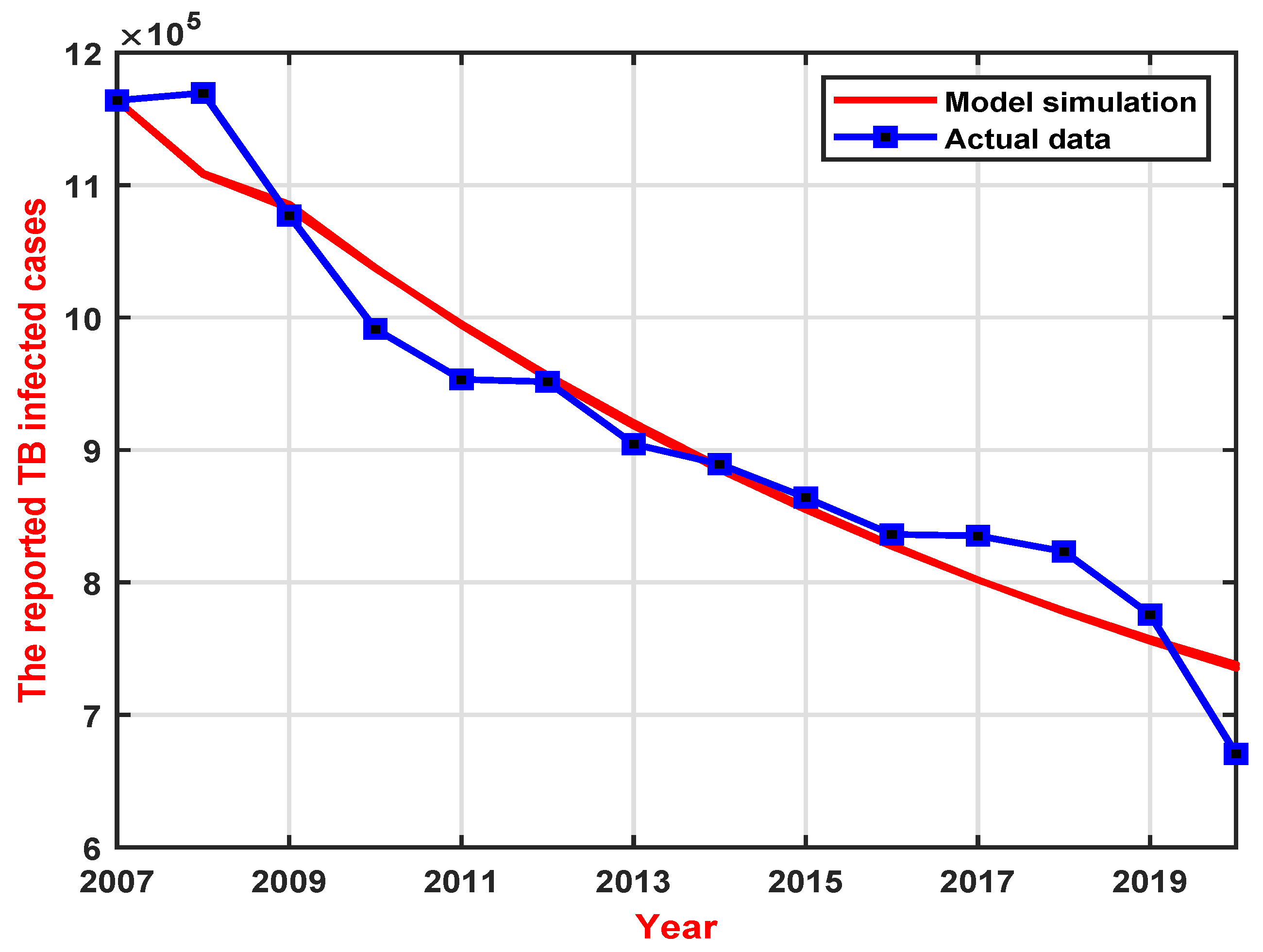
Next, we utilize P ( t , Θ ^ ) to simulate China’s annual tuberculosis patient data. We use MATLAB 2018b software to estimate Θ ^ . Using the Grey Wolf Optimizer (GWO) algorithm, we can estimate the unknown parameters and initial values for model (1), as shown in Table 3. The results of the simulation are presented in Figure 2.

5.2. Sensitivity Analysis

The output of the model (1) is determined by its initial values and parameters. The GWO algorithm is used to estimate some parameters and initial values, which may introduce uncertainty into their selection. Therefore, we need to conduct an uncertainty analysis (UA) in order to determine the reliability of parameter estimates. To ensure the reliability of the estimates through the GWO, we employ the Markov Chain Monte Carlo (MCMC) method with the Delayed Rejection and Adaptive Metropolis (DRAM) algorithm [40]. We estimate the convergence of the Markov chain by using Geweke’s Z-scores [41]. The expectations, standard deviations, and confidence intervals of the parameters and initial values are listed in Table 4.
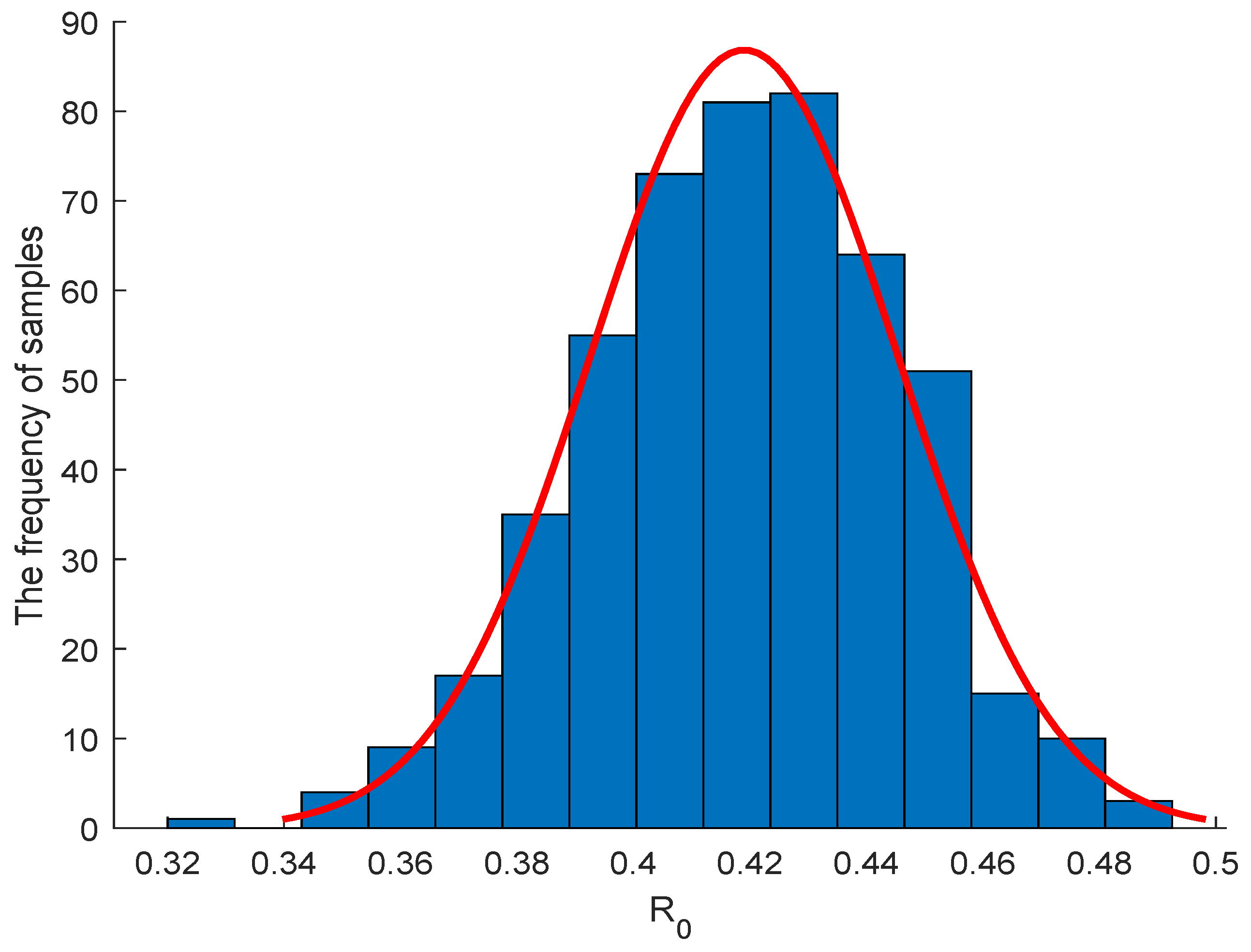
In this paper, a sensitivity analysis (SA) is used to identify the parameter that has the greatest impact on R 0 . We use the partial rank correlation coefficient (PRCC) to analyze the sensitivity, which is based on Latin hypercube sampling (LHS). For the parameters presented in Table 4, we let m 1 , V ( 0 ) take the expected value, and we assume that other parameters follow normal distributions with the expectations and standard deviations shown in Table 4. Because the parameters are sampled normally, we can observe that the distribution of R 0 is also normal in Figure 3. Figure 3 shows that the average of R 0 < 1 . It follows from Theorem 7 that the model 1 is globally asymptotically stable to the disease-free equilibrium state, which suggests that TB transmission will eventually disappear. However, this does not mean that China will achieve the End TB Strategy of the WHO (reducing the incidence of TB by 90 % by 2035 compared to 2015) [1,2]. Thus, China should find the most effective measures to achieve the goal of the WHO. Figure 4 shows the values of PRCC for R 0 . It follows from the values of PRCC that δ ( a ) , β , α , and γ have significant influences on R 0 .

6. Discussion and Conclusions

The rate δ ( a ) at which latent individuals enter the infectious class has a significant influence on R 0 . But, we think it is difficult to implement control measures on the parameter in China’s public health at present. The parameter α represents the relapse rate. If the relapse rate α is reduced, we can see a significant reduction in R 0 , which will lead to a significant reduction in the number of new cases. Therefore, gaining a better understanding of the causes and risk factors associated with TB relapse is crucial for controlling the spread of TB in China. The TB transmission coefficient β has a significant impact on R 0 . To decrease β , effort is needed to prevent susceptible populations from becoming TB latent populations. This includes paying attention to personal protection, accepting TB treatment and prevention education, avoiding unhealthy living habits, and more. The treatment rate γ exerts a significant influence on R 0 . To increase γ , efforts are needed to expand the coverage of TB treatment and improve treatment success rates for patients with TB disease. Therefore, implementing these measures could effectively reduce the TB incidence rate in China. However, we also found that the waning rate ω of vaccine-induced protection has no significant effect on R 0 . We suggest that this does not necessarily mean that the BCG vaccine has no effect on preventing and controlling TB. The possible reason for this is that we assumed a fixed efficacy rate for the vaccine in the simulation. If the vaccine’s effectiveness were improved, it would be possible to significantly reduce the number of new TB cases. Therefore, the development of novel vaccines is also a focal point for the goal of TB control.
In this paper, we present an age-structured mathematical model for TB infection based on the characteristics of TB transmission in order to gain a better understanding of the spread of TB in China. The aim of our research was to propose control strategies to mitigate the risk of TB spread. We defined the basic reproduction number R 0 and demonstrated that it is the key determinant of the global dynamics in our proposed model. Based on annual data on TB in China collected from 2007 to 2020, we estimated the model parameters and calculated the PRCC between these parameters and the basic reproduction number R 0 . From the PRCC values, we can see that δ ( a ) , β , α , and γ have the most important influences on R 0 . In light of the actual controllability, we proposed some measures to control the spread of TB in China. There are still some deficiencies in our study. Firstly, we did not take into account the time lag caused by treatment in our modeling, which may pose great difficulties for the dynamic analysis of the model. Secondly, we did not consider drug resistance, as the treatment success rate for patients with drug resistance is significantly lower. Thirdly, the distributions of δ ( a ) and σ ( a ) are based on our hypothesis and will be studied further when relevant data become publicly available.

Author Contributions

Z.G. carried out the methodology, investigation, and writing of the draft. L.Z. supervised the research and reviewed the final draft. All authors have read and agreed to the published version of the manuscript.

Funding

This research was supported by Natural Science Foundation of Gansu of China (Grant No. 22JR5RA350, No. 22JR5RA337).

Institutional Review Board Statement

Not applicable.

Informed Consent Statement

Not applicable.

Data Availability Statement

Not applicable.

Acknowledgments

We wish to thank the reviewers, whose careful reading and comments greatly improved the paper.

Conflicts of Interest

The authors declare no conflict of interest.

References

  1. WHO. Global Tuberculosis Report 2022. Available online: https://www.who.int/publications/i/item/9789240061729 (accessed on 5 April 2023).
  2. Guo, Z.K.; Xiang, H.; Huo, H.F. Analysis of an age-structured tuberculosis model with treatment and relapse. J. Math. Biol. 2021, 82, 45. [Google Scholar] [CrossRef] [PubMed]
  3. Das, D.K.; Khajanchi, S.; Kar, T. Transmission dynamics of tuberculosis with multiple re-infections. Chaos Solitons Fractals 2020, 130, 109450. [Google Scholar] [CrossRef]
  4. Choi, S.; Jung, E.; Lee, S.M. Optimal intervention strategy for prevention tuberculosis using a smoking-tuberculosis model. J. Theor. Biol. 2015, 380, 256–270. [Google Scholar] [CrossRef] [PubMed]
  5. Liu, Q.; Jiang, D. The dynamics of a stochastic vaccinated tuberculosis model with treatment. Phys. A Stat. Mech. Appl. 2019, 527, 121274. [Google Scholar] [CrossRef]
  6. Ozcaglar, C.; Shabbeer, A.; Vandenberg, S.L.; Yener, B.; Bennett, K.P. Epidemiological models of Mycobacterium tuberculosis complex infections. Math. Biosci. 2012, 236, 77–96. [Google Scholar] [CrossRef] [PubMed]
  7. Choi, S.; Jung, E. Optimal Tuberculosis Prevention and Control Strategy from a Mathematical Model Based on Real Data. Bull. Math. Biol. 2014, 76, 1566–1589. [Google Scholar] [CrossRef] [PubMed]
  8. Huo, H.F.; Zou, M.X. Modelling effects of treatment at home on tuberculosis transmission dynamics. Appl. Math. Model. 2016, 40, 9474–9484. [Google Scholar] [CrossRef]
  9. Zhang, W. Analysis of an in-host tuberculosis model for disease control. Appl. Math. Lett. 2020, 99, 105983. [Google Scholar] [CrossRef]
  10. CDC. Basic TB Facts. Available online: https://www.cdc.gov/tb/topic/basics/default.htm (accessed on 5 April 2023).
  11. Burman, W.J.; Bliven, E.E.; Cowan, L.; Bozeman, L.; Nahid, P.; Diem, L.; Vernon, A. Relapse associated with active disease caused by Beijing strain of Mycobacterium tuberculosis. Emerg. Infect. Dis. 2009, 15, 1061–1067. [Google Scholar] [CrossRef]
  12. Trollfors, B.; Sigurdsson, V.; Dahlgren-Aronsson, A. Prevalence of Latent TB and Effectiveness of BCG Vaccination Against Latent Tuberculosis: An Observational Study. Int. J. Infect. Dis. 2021, 109, 279–282. [Google Scholar] [CrossRef]
  13. Martinez, L.; Cords, O.; Liu, Q.; Acuna-Villaorduna, C.; Bonnet, M.; Fox, G.J.; Carvalho, A.C.C.; Chan, P.C.; Croda, J.; Hill, P.C.; et al. Infant BCG vaccination and risk of pulmonary and extrapulmonary tuberculosis throughout the life course: A systematic review and individual participant data meta-analysis. Lancet Glob. Health 2022, 10, e1307–e1316. [Google Scholar] [CrossRef] [PubMed]
  14. Setiabudiawan, T.P.; Reurink, R.K.; Hill, P.C.; Netea, M.G.; van Crevel, R.; Koeken, V.A. Protection against tuberculosis by Bacillus Calmette-Guérin (BCG) vaccination: A historical perspective. Med 2022, 3, 6–24. [Google Scholar] [CrossRef] [PubMed]
  15. Kerantzas, C.A.; Jacobs, W.R. Origins of Combination Therapy for Tuberculosis: Lessons for Future Antimicrobial Development and Application. mBio 2017, 8. [Google Scholar] [CrossRef] [PubMed]
  16. Hosseiniporgham, S.; Sechi, L.A. A Review on Mycobacteriophages: From Classification to Applications. Pathogens 2022, 11, 777. [Google Scholar] [CrossRef] [PubMed]
  17. WHO. Tuberculosis: Multidrug-Resistant Tuberculosis (MDR-TB). Available online: https://www.who.int/news-room/questions-and-answers/item/tuberculosis-multidrug-resistant-tuberculosis-(mdr-tb) (accessed on 29 July 2023).
  18. Li, Y.; Liu, X.; Yuan, Y.; Li, J.; Wang, L. Global analysis of tuberculosis dynamical model and optimal control strategies based on case data in the United States. Appl. Math. Comput. 2022, 422, 126983. [Google Scholar] [CrossRef]
  19. Ren, S. Global stability in a tuberculosis model of imperfect treatment with age-dependent latency and relapse. Math. Biosci. Eng. 2017, 14, 1337–1360. [Google Scholar] [CrossRef]
  20. Iannelli, M.; Milner, F. The Basic Approach to Age-Structured Population Dynamics; Springer Nature: Dordrecht, The Netherlands, 2017. [Google Scholar]
  21. Guo, Z.K.; Huo, H.F.; Xiang, H. Analysis of an age-structured model for HIV-TB co-infection. Discret. Contin. Dyn. Syst. 2022, 27, 199–228. [Google Scholar] [CrossRef]
  22. Guo, Z.K.; Huo, H.F.; Xiang, H. Global dynamics of an age-structured malaria model with prevention. Math. Biosci. Eng. 2019, 16, 1625–1653. [Google Scholar] [CrossRef]
  23. Inaba, H.; Sekine, H. A mathematical model for Chagas disease with infection-age-dependent infectivity. Math. Biosci. 2004, 190, 39–69. [Google Scholar] [CrossRef]
  24. Ghosh, I.; Tiwari, P.K.; Samanta, S.; Elmojtaba, I.M.; Al-Salti, N.; Chattopadhyay, J. A simple SI-type model for HIV/AIDS with media and self-imposed psychological fear. Math. Biosci. 2018, 306, 160–169. [Google Scholar] [CrossRef]
  25. Li, T.; Zhang, F.; Liu, H.; Chen, Y. Threshold dynamics of an SIRS model with nonlinear incidence rate and transfer from infectious to susceptible. Appl. Math. Lett. 2017, 70, 52–57. [Google Scholar] [CrossRef]
  26. Sigdel, R.P.; McCluskey, C.C. Global stability for an SEI model of infectious disease with immigration. Appl. Math. Comput. 2014, 243, 684–689. [Google Scholar] [CrossRef]
  27. Wang, L.; Liu, Z.; Zhang, X. Global dynamics for an age-structured epidemic model with media impact and incomplete vaccination. Nonlinear Anal. Real World Appl. 2016, 32, 136–158. [Google Scholar] [CrossRef]
  28. Chen, Y.; Zou, S.; Yang, J. Global analysis of an SIR epidemic model with infection age and saturated incidence. Nonlinear Anal. Real World Appl. 2016, 30, 16–31. [Google Scholar] [CrossRef]
  29. Smith, H.L.; Thieme, H.R. Dynamical Systems and Population Persistence; American Mathematical Society: Providence, RI, USA, 2011. [Google Scholar]
  30. Magal, P.; Zhao, X.Q. Global Attractors and Steady States for Uniformly Persistent Dynamical Systems. SIAM J. Math. Anal. 2005, 37, 251–275. [Google Scholar] [CrossRef]
  31. Hale, J.K.; Waltman, P. Persistence in Infinite-Dimensional Systems. SIAM J. Math. Anal. 1989, 20, 388–395. [Google Scholar] [CrossRef]
  32. Browne, C.J.; Pilyugin, S.S. Global analysis of age-structured within-host virus model. Discret. Contin. Dyn. Syst. Ser. B 2013, 18, 1999–2017. [Google Scholar] [CrossRef]
  33. Lasalle, J.P. Some Extensions of Liapunov’s Second Method. Ire Trans. Circuit Theory 1960, 7, 520–527. [Google Scholar] [CrossRef]
  34. World Health Organization. Available online: https://www.who.int/health-topics/tuberculosis#tab=tab_1 (accessed on 18 August 2023).
  35. Centers for Disease Control and Prevention. Available online: https://www.cdc.gov/tb/ (accessed on 18 August 2023).
  36. National Bureau of Statistics of China. Available online: http://www.stats.gov.cn/ (accessed on 18 August 2023).
  37. Xue, L.; Jing, S.; Wang, H. Evaluating Strategies For Tuberculosis to Achieve the Goals of WHO in China: A Seasonal Age-Structured Model Study. Bull. Math. Biol. 2022, 84, 1–50. [Google Scholar] [CrossRef]
  38. Huang, W.; Fang, Z.; Luo, S.; Lin, S.; Xu, L.; Yan, B.; Liu, X.; Xia, L.; Fan, X.; Lu, S. The effect of BCG vaccination and risk factors for latent tuberculosis infection among college freshmen in China. Int. J. Infect. Dis. 2022, 122, 321–326. [Google Scholar] [CrossRef]
  39. Chinese Center for Disease Control and Prevention. Available online: http://www.chinacdc.cn/ (accessed on 18 August 2023).
  40. Haario, H.; Laine, M.; Mira, A.; Saksman, E. DRAM: Efficient adaptive MCMC. Stat. Comput. 2006, 16, 339–354. [Google Scholar] [CrossRef]
  41. MCMC Toolbox for Matlab. Available online: https://mjlaine.github.io/mcmcstat/index.html#org0701d35 (accessed on 18 August 2023).
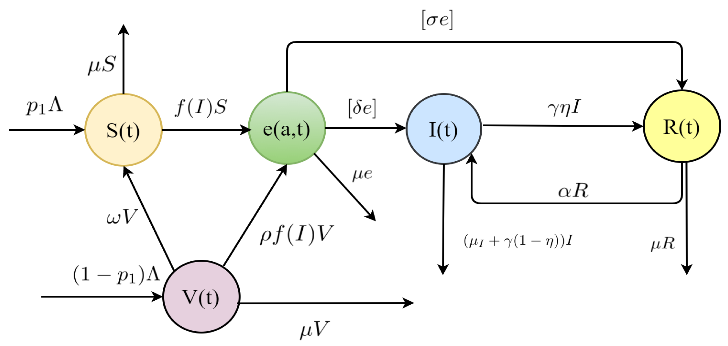
Figure 1. Flowchart of the transmission of TB.
Axioms 12 00805 g001
Figure 2. The comparison between the simulation results of the GWO algorithm and the actual data.
Axioms 12 00805 g002
Figure 3. The distribution histogram of R 0 .
Axioms 12 00805 g003
Figure 4. The PRCC values.
Axioms 12 00805 g004
Table 1. The parameters’ meanings in the model (1).
NotationsDefinitions
Λ the rate of recruitment of susceptible individuals
μ the constant natural death rate of individuals in every compartment
1 p 1 the coverage rate of the BCG vaccine
ω the rate of vaccine-induced protection wanes
ρ the reduction coefficient of the contagion rate
δ ( a ) the rate distribution of latent individuals entering the infectious subclass
σ ( a ) the rate distribution of latent individuals entering the recovered subclass
γ the rate of treatment
μ I the death rate of the infectious individuals
η the proportion of effective treatment
α the relapse rate
Table 2. The data of TB cases in China (persons).
Year2007200820092010201120122013
Cases1,163,9591,169,5401,076,938991,350953,275951,508904,434
Year2014201520162017201820192020
Cases889,381864,015836,236835,193823,342775,764670,538
Table 3. Unknown parameters and initial values estimated by the GWO algorithm.
ParametersValueSourceParametersValueSource
δ 1 0.01518682Fitting β 1 2.8311140 × 10 12 Fitting
δ 2 0.047465098Fitting m 1 1,805,707Fitting
σ 1 0.086799875Fitting α 0.010890517Fitting
σ 2 0.000960051Fitting γ 0.200034765Fitting
ω 0.090614519 Fitting V ( 0 ) 129,832,691Fitting
β 4.887090 × 10 11
Table 4. The parameters and initial values of the model (1).
ParametersMeanStd95% CIGewekes Z-Score
δ 1 0.0152240.0017461[0.01521682, 0.015232125]0.99492
δ 2 0.0473570.0054654[0.047333118, 0.047381024]0.9904
σ 1 0.086930.010083[0.0868855, 0.086973908]0.98351
σ 2 0.000959030.00011069[0.000958544, 0.000959514]0.99975
ω 0.0907250.010535[0.090678698, 0.09077104]0.99583
β 4.8889 × 10 11 5.6062 × 10 12 [ 4.88647 × 10 11 , 4.891385 × 10 11 ] 0.99636
β 1 2.824 × 10 12 3.2717 × 10 13 [ 2.82254 × 10 12 , 2.825412 × 10 12 ] 0.98896
m 1 1,801,600209,190[1,800,674, 1,802,508]0.99182
α 0.0108820.0012476[0.010876, 0.010887]0.98807
γ 0.199720.023108[0.1996197, 0.199822]0.9752
V ( 0 ) 13 , 038 , 000 1.5 × 10 7 [130,309,596, 130,441,079]0.99426
Disclaimer/Publisher’s Note: The statements, opinions and data contained in all publications are solely those of the individual author(s) and contributor(s) and not of MDPI and/or the editor(s). MDPI and/or the editor(s) disclaim responsibility for any injury to people or property resulting from any ideas, methods, instructions or products referred to in the content.