Extropy Based on Concomitants of Order Statistics in Farlie-Gumbel-Morgenstern Family for Random Variables Representing Past Life

Abstract

In this paper, we refined the concept of past extropy measure for concomitants of order statistics from Farlie-Gumbel-Morgenstern family. In addition, cumulative past extropy measure and dynamic cumulative past extropy measure for concomitant of rth order statistic are also conferred and their properties are studied. The problem of estimating the cumulative past extropy is investigated using empirical technique. The validity of the proposed estimator has been emphasized using simulation study.

1. Introduction

Let $(X_i,Y_i)$, $i=1,2,\dots ,n$ be independent and identically distributed (iid) random variables (rvs) from a continuous bivariate distribution with cumulative distribution function (cdf) $F(x,y)$ and joint probability density function (pdf) $f(x,y)$. Let $f_X\left(x\right)$ and $f_Y\left(y\right)$ be the marginal pdf of X and Y respectively, $F_X\left(x\right)$ and $F_Y\left(y\right)$ be the marginal cdf, respectively. We define $F_Y^{-1}\left(u\right)=inf\left\{y;F_Y\left(y\right)\ge u\right\},u\in \left[0,1\right]$ as the quantile function of $F_Y\left(y\right)$. If we arrange $Xs$ in the order $X_1\le X_2\le \dots \dots \le X_n$, then the $Ys$ associated with these order statistics (OS) are called concomitants of order statistics (COS). We denote $X_{r:n}$ and $Y_{[r:n]}$ for the rth order statistic and concomitant of rth order statistic.

If the members of a random sample are sorted according to corresponding values of an other random sample, then the COS arise. The concept of COS has been introduced by [1]. It has important applications in various areas such as in selection problems, inference problems etc. One may refer [2] for more details and applications of COS.

The common approach in the problems of modeling is that to select a family of distributions and then choose the one from the family that is more appropriate to describe the observation. The desirable feature of selecting a family is that it should be flexible. That is, it should accommodate several models that could represent any data situations. The most well-known parametric family from all the available parametric families is the Farlie-Gumbel-Morgenstern (FGM) family, that is mannered by [3]. The FGM family of distributions is constructed in such a way that it includes a joint distribution function along with its marginals, which makes it easier for the analyst to make several assumptions about marginals. Ref. [4] studied about the new generalized FGM distributions and COS. A multi-parameter Generalized FGM bivariate copula family via Bernstein polynomial has been introduced by [5].

One of the most widely used measure of uncertainty is the entropy measure introduced by [6], which is used to quantify the amount of uncertainty involved in a rv and has several applications in various areas. The Shannon entropy is given by

$$H\left(X\right)=-{\int }_0^{\infty }{f}_X\left(x\right)log{f}_X\left(x\right)dx.$$

Interested readers can refer the work by [7] for the characterizations of OS and records of entropy. Ref. [8] introduced new measure of sample entropy of continuous rv. Ref. [9] suggested some estimators of entropy using random sampling. The idea of varentropy is proposed by [10] as a great replacement for the kurtosis measure.

The differential extropy proposed by [11] is considered as the complementary dual of Shannon entropy. It is appeared from a critical analysis to score the forecasting distribution. For a non-negative rv X with pdf $f_X\left(x\right)$, differential extropy is given as follows

$$J\left(X\right)=-\frac{1}{2}{\int }_0^{\infty }{f}_X^2\left(x\right)dx.$$

(1)

In the application perspective, one can refer to [12] for the application of extropy in thermodynamics and [13] for the application of extropy in automatic speech recognition. Ref. [14] analysed the characterization results of extropy using OS and record values. Ref. [15] developed some results related to extropy properties of mixed systems. Ref. [16] provided general weighted extropy of ranked set sampling (RSS). They studied some characterization results, stochastic comparison and monotone properties of general weighted extropy.

In order to deal with the situations where uncertainty may be confined to the past life of an event, ref. [17] introduced past entropy for a rv ${}_{t}X=\left(t-x|X<t\right)$. The past extropy is offered by [18,19] to measure the uncertainty in a past lifetime distribution based on extropy. It is given as

$$J_t\left(X\right)=-\frac{1}{2}{\int }_0^t{\left(\frac{f_X\left(x\right)}{F_X\left(t\right)}\right)}^{2}dx.$$

(2)

From Equation (2), it is clear that $J_t\left(X\right)<0$ and $J_t\left(X\right)=J\left(X\right)$, for $t=\infty$. It has several applications in information theory, reliability theory, survival analysis etc.

Ref. [20] introduced the concept of varextropy which is a dispersion measure of extropy for residual and past lifetimes of rvs. Ref. [21] explored RSS properties of past extropy and negative cumulative extropy. Ref. [22] made a comparison study between past entropy and past extropy and showed that there are situations where uncertainty related to past life is approximately lower for past extropy measure than past entropy. Thus, it is evident that in some situations of uncertainty, information content is more while using past extropy measure than past entropy for rvs representing past life time.

If the properties of the residual and past lifetime depend on time, they are considered as dynamic. This means that these characteristics vary over time and are not constant. Ref. [23] considered dynamic weighted extropy. Ref. [24] introduced the concept of dynamic survival extropy in the literature. Ref. [25] introduced another uncertainty measure called Dynamic survival past extropy (DSPE) for past lifetime of a system. It is defined for a non-negative rv X with absolutely continuous cdf $F_X\left(x\right)$ as

$$J_{DS{P}_t}\left(X\right)=-\frac{1}{2}{\int }_0^t{\left(\frac{F_X\left(x\right)}{F_X\left(t\right)}\right)}^{2}dx.$$

(3)

It is always less than zero and for $t=\infty$, it became the cumulative past extropy (CPE) which is given by [25], as

$${ℐ}_t=-\frac{1}{2}{\int }_0^{\infty }{F}_X^2\left(x\right)dx.$$

(4)

Some properties of Fisher information in OS and its concomitants are inspected by [26]. Ref. [27] explored information properties for COS in FGM family. [28] explored properties of extropy for concomitants of generalized OS in FGM family. Ref. [29] explained the concept of ordered variables and their concomitants under extropy via COVID-19 data application. Ref. [30] developed the approach of the extropy of concomitants of generalized OS from Huang–Kotz–Morgenstern bivariate distribution.

The concomitants are mostly used in selection problems where the individuals are chosen according to the X values and associated characteristic is shown using the corresponding the Y values. The flexible nature of the FGM family is built in such a way that once the prior information in the form of marginals is available the bivariate distribution can be constructed with the help of those marginals and correlation between the variables directly. Its flexibility encouraged us to cope up the work in COS from FGM family. Ref. [31] studied residual and past entropy for concomitants of ordered rvs from FGM family. But not any work is available on the literature based on the COS from FGM family in the case of past life time rvs. This motivated us to present the information content and properties of COS for the rvs representing past lifetime.

The structure of the paper is organized as: In Section 2, we obtain the expression for $Y_{[r:n]}$ based on past extropy measure as well as some results related to past extropy of concomitant of rth order statistic are derived. In Section 3 and Section 4, the properties of COS in CPE and DSPE measures are studied. Section 5 deals with the estimation of CPE for concomitant of rth order statistic using empirical estimators. And in Section 6, simulation study is exhibited to support the potency of the estimator. Finally, Section 7 provides a conclusion of main findings.

2. Past Extropy for Concomitants of Order Statistics in FGM Family

In this section, we derive measures of past extropy for COS in FGM family.

The cdf and pdf of the FGM family are given by [32] as

$$F_{X,Y}(x,y)=F_X\left(x\right)F_Y\left(y\right)[1+\alpha (1-F_X\left(x\right))(1-F_Y\left(y\right))],$$

(5)

and

$$f_{X,Y}(x,y)=f_X\left(x\right)f_Y\left(y\right)[1+\alpha (2F_X\left(x\right)-1)\left(2F_Y\left(y\right)\right)-1],$$

(6)

where $-1\le \alpha \le 1$, $f_X\left(x\right)$ and $f_Y\left(y\right)$ are the marginal pdf of X and Y, respectively. $F_X\left(x\right)$ and $F_Y\left(y\right)$ are the marginal cdf of X and Y, respectively.

The pdf and cdf of concomitant of $r$th order statistic $Y_{[r:n]}$ given by [33], respectively are

$$g_{Y_{[r:n]}}=f_Y\left(y\right)\left[1+{\gamma }_r\left(1-2F_Y\left(y\right)\right)\right],$$

(7)

and

$$G_{Y_{[r:n]}}\left(y\right)=F_Y\left(y\right)\left[1+{\gamma }_r\left(1-F_Y\left(y\right)\right)\right],$$

(8)

where ${\gamma }_r=\alpha \frac{n-2r+1}{n+1}$.

Proposition 1.

Let $(X_i,Y_i)$, $i=1,2,\cdots ,n$ be a bivariate random sample from FGM family and $Y_{[r:n]}$ denotes the concomitant of the rth order statistic arising from FGM family, the past extropy of $Y_{[r:n]}$ denoted as $J_t\left(Y_{[r:n]}\right)$ is given by

$$\begin{array}{c}\hfill J_t\left(Y_{[r:n]}\right)={\left(\frac{1}{1+{\gamma }_r(1-F_Y\left(t\right))}\right)}^2[{\left(1+{\gamma }_r\right)}^2{J}_t\left(Y\right)+\frac{2{\gamma }_r\left(1+{\gamma }_r\right)}{F_Y\left(t\right)}E\left(U_t{f}_Y\left(F_Y^{-1}\left(U_t\right)\right)\right)\\ \hfill -\frac{2{\gamma }_r^2}{F_Y\left(t\right)}E\left(U_t^2{f}_Y\left(F_Y^{-1}\left(U_t\right)\right)\right)],\end{array}$$

(9)

where $J_t\left(Y\right)$ is the past extropy of rv Y, ${\gamma }_r=\alpha \frac{n-2r+1}{n+1}$ and $U_t$ is a uniformly distributed rv on $(0,F_Y\left(t\right))$ with pdf $\frac{1}{F_Y\left(t\right)}$.

Proof. 

For $Y_{[r:n]}$, from Equation (2) we have

$$J_t\left(Y_{[r:n]}\right)=-\frac{1}{2}{\int }_0^t\frac{g_{Y_{[r:n]}}^2\left(y\right)}{G_{Y_{[r:n]}}^2\left(t\right)}dy,$$

(10)

where $g_{Y_{[r:n]}}$ and $G_{Y_{[r:n]}}$ are defined in Equations (7) and (8), respectively.

Then,

$$\begin{array}{cc}\hfill J_t\left(Y_{[r:n]}\right)& =-\frac{1}{2}{\int }_0^t\frac{f_Y^2\left(y\right){\left[1+{\gamma }_r\left(1-2F_Y\left(y\right)\right)\right]}^2}{G_{Y_{[r:n]}}^2\left(t\right)}dy\hfill \\ \hfill & =-\frac{1}{2}{\int }_0^t\frac{f_Y^2\left(y\right)\left[1+2{\gamma }_r(1-2F_Y\left(y\right))+{\gamma }_r^2{\left(1-2F_Y\left(y\right)\right)}^2\right]}{G_{Y_{[r:n]}}^2\left(t\right)}dy\hfill \\ \hfill & =-\frac{1}{2}{\int }_0^t\frac{f_Y^2\left(y\right)[1+2{\gamma }_r(1-2F_Y\left(y\right))+{\gamma }_r^2(1-4F_Y\left(y\right)+4F_Y^2\left(y\right))]}{G_{Y_{[r:n]}}^2\left(t\right)}dy.\hfill \end{array}$$

Expanding and rearranging, we get

$$\begin{array}{c}\hfill J_t\left(Y_{[r:n]}\right)=-\frac{1}{2G_{Y_{[r:n]}}^2\left(t\right)}[{(1+{\gamma }_r)}^2{\int }_0^t{f}_Y^2\left(y\right)dy-4{\gamma }_r(1+{\gamma }_r){\int }_0^t{F}_Y\left(y\right)f_Y^2\left(y\right)dy\\ \hfill +4{\gamma }_r^2{\int }_0^t{F}_Y^2\left(y\right)f_Y^2\left(y\right)dy].\end{array}$$

Using Equation (8) it will be

$$\begin{array}{cc}\hfill J_t\left(Y_{[r:n]}\right)=& -\frac{1}{2}{\left(\frac{1}{1+{\gamma }_r(1-F_Y\left(t\right))}\right)}^2[\frac{{(1+{\gamma }_r)}^2}{F_Y^2\left(t\right)}{\int }_0^t{f}_Y^2\left(y\right)dy\hfill \\ \hfill & -\frac{4{\gamma }_r(1+{\gamma }_r)}{F_Y^2\left(t\right)}{\int }_0^t{F}_Y\left(y\right)f_Y^2\left(y\right)dy+\frac{4{\gamma }_r^2}{F_Y^2\left(t\right)}{\int }_0^t{F}_Y^2\left(y\right)f_Y^2\left(y\right)dy]\hfill \\ \hfill =& {\left(\frac{1}{1+{\gamma }_r(1-F_Y\left(t\right))}\right)}^2[-\frac{{(1+{\gamma }_r)}^2}{2F_Y^2\left(t\right)}{\int }_0^{F_Y\left(t\right)}{f}_Y\left(F_Y^{-1}\left(u\right)\right)du\hfill \\ \hfill & +\frac{2{\gamma }_r(1+{\gamma }_r)}{F_Y^2\left(t\right)}{\int }_0^{F_Y\left(t\right)}u{f}_Y\left(F_Y^{-1}\left(u\right)\right)du-\frac{2{\gamma }_r^2}{F_Y^2\left(t\right)}{\int }_0^{F_Y\left(t\right)}{u}^2{f}_Y\left(F_Y^{-1}\left(u\right)\right)du]\hfill \\ \hfill =& {\left(\frac{1}{1+{\gamma }_r(1-F_Y\left(t\right))}\right)}^2[{\left(1+{\gamma }_r\right)}^2{J}_t\left(Y\right)+\frac{2{\gamma }_r(1+{\gamma }_r)}{F_Y^2\left(t\right)}{\int }_0^{F_Y\left(t\right)}u{f}_Y\left(F_Y^{-1}\left(u\right)\right)du\hfill \\ \hfill & -\frac{2{\gamma }_r^2}{F_Y^2\left(t\right)}{\int }_0^{F_Y\left(t\right)}{u}^2{f}_Y\left(F_Y^{-1}\left(u\right)\right)du]\hfill \\ \hfill =& {\left(\frac{1}{1+{\gamma }_r(1-F_Y\left(t\right))}\right)}^2[{\left(1+{\gamma }_r\right)}^2{J}_t\left(Y\right)+\frac{2{\gamma }_r\left(1+{\gamma }_r\right)}{F_Y\left(t\right)}E\left(U_t{f}_Y\left(F_Y^{-1}\left(U_t\right)\right)\right)\hfill \\ \hfill & -\frac{2{\gamma }_r^2}{F_Y\left(t\right)}E\left(U_t^2{f}_Y\left(F_Y^{-1}\left(U_t\right)\right)\right)].\hfill \end{array}$$

Hence, the theorem is proved. □

Remark 1.

When $\alpha =0$ in Equation (9), then ${\gamma }_r=0$, which implies $J_t\left(Y_{[r:n]}\right)=J_t\left(Y\right)$.

Remark 2.

If $r=1$ and $r=n$, we get the concomitants of the 1st and nth OS of a random sample of size n. Then, the past extropy measure for COS $Y_{[1:n]}$ and $Y_{[n:n]}$, respectively are given by

$$\begin{array}{cc}\hfill J_t\left(Y_{[1:n]}\right)& ={\left(\frac{1}{1+C_{n,\alpha }(1-F_Y\left(t\right))}\right)}^2\left[{\left(1+C_{n,\alpha }\right)}^2{J}_t\left(Y\right)\right.\hfill \\ \hfill & \left.+\frac{2C_{n,\alpha }\left(1-C_{n,\alpha }\right)}{F_Y\left(t\right)}E\left(U_t{f}_Y\left(F_Y^{-1}\left(U_t\right)\right)\right)-\frac{2C_{n,\alpha }^2}{F_Y\left(t\right)}E\left(U_t^2{f}_Y\left(F_Y^{-1}\left(U_t\right)\right)\right)\right],\hfill \end{array}$$

(11)

and

$$\begin{array}{cc}\hfill J_t\left(Y_{[n:n]}\right)& ={\left(\frac{1}{1-C_{n,\alpha }(1-F_Y\left(t\right))}\right)}^2\left[{\left(1-C_{n,\alpha }\right)}^2{J}_t\left(Y\right)\right.\hfill \\ \hfill & \left.-\frac{2C_{n,\alpha }\left(1-C_{n,\alpha }\right)}{F_Y\left(t\right)}E\left(U_t{f}_Y\left(F_Y^{-1}\left(U_t\right)\right)\right)-\frac{2C_{n,\alpha }^2}{F_Y\left(t\right)}E\left(U_t^2{f}_Y\left(F_Y^{-1}\left(U_t\right)\right)\right)\right],\hfill \end{array}$$

(12)

where $U_t$ is a rv distributed uniformly on $(0,F_Y\left(t\right))$ and $C_{n,\alpha }=\alpha \frac{n-1}{n+1}$.

Example 1.

Let $(X_i,Y_i)$, $i=1,2,\dots ,n$ be a bivariate random sample arising from FGM bivariate exponential distribution with cdf

$$F(x,y)=\left(1-e^{-\frac{x}{{\theta }_1}}\right)\left(1-e^{-\frac{y}{{\theta }_2}}\right)\left(1+\alpha e^{-\frac{x}{{\theta }_1}-\frac{y}{{\theta }_2}}\right),$$

(13)

where $-1\le \alpha \le 1,$ $x,y>0$, ${\theta }_1,{\theta }_2>0$. Then,

$$J_t\left(Y_{[r:n]}\right)=-\frac{-2e^{-\frac{t}{{\theta }_2}}(-4+{\gamma }_r){\gamma }_r+6{\gamma }_r^2+e^{\frac{2t}{{\theta }_2}}(3+{\gamma }_r(2+{\gamma }_r))+e^{\frac{3t}{{\theta }_2}}(3+{\gamma }_r(2+{\gamma }_r))}{12(-1+e^{\frac{t}{{\theta }_2}}){\theta }_2{(e^{\frac{t}{{\theta }_2}}+{\gamma }_r)}^2}.$$

(14)

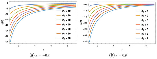
Figure 1 shows some plots of $J_t\left(Y_{[r:n]}\right)$ for a sample of size $n=50$ and the first order statistic $r=1$ with various selections of ${\theta }_2$ for FGM bivariate exponential distribution.

Figure 1. The plots of $J_t\left(Y_{[r:n]}\right)$ for $n=50,r=1$ with various values of ${\theta }_2$ for FGM bivariate exponential distribution.

It is clear that $J_t\left(Y_{[r:n]}\right)$ values are negative for all cases considered in this figure. Using Equation (14), the difference between concomitants of nth and 1st OS for past extropy measure denoted as $D_t$ is given by

$$\begin{array}{cc}\hfill D_t& =J_t\left(Y_{[n:n]}\right)-J_t\left(Y_{[1:n]}\right)\hfill \\ \hfill & =\frac{e^{\frac{t}{{\theta }_2}}(-1+e^{\frac{t}{{\theta }_2}})(-1+n^2)\alpha \left[e^{\frac{t}{{\theta }_2}}{(1+n)}^2-2{(-1+n)}^2{\alpha }^2-e^{\frac{t}{{\theta }_2}}{(-1+n)}^2{\alpha }^2\right]}{3{\left[e^{\frac{2t}{{\theta }_2}}{(1+n)}^2-{(-1+n)}^2{\alpha }^2\right]}^2{\theta }_2},\hfill \end{array}$$

(15)

which is positive when $0<\alpha \le 1$, is negative when $-1\le \alpha <0$, and is zero for $\alpha =0$.

Example 2.

For FGM bivariate logistic distribution with cdf

$$F(x,y)={\left(1+e^{-x}\right)}^{-1}{\left(1+e^{-y}\right)}^{-1}\left(1+\alpha \frac{e^{-x-y}}{\left(1+e^{-x}\right)\left(1+e^{-y}\right)}\right),$$

(16)

where $-1\le \alpha \le 1$, $-\infty <x<\infty$ and $-\infty <y<\infty$, the past extropy is given by

$$\begin{array}{c}\hfill J_t\left(Y_{[r:n]}\right)=-\frac{e^{-2t}\left(-1+e^t\right)}{480\left(1+e^t\right)\left(1+e^t+{\gamma }_r^2\right)}\left(20+120e^t+200e^{2t}+120e^{3t}+20e^{4t}+15{\gamma }_r\right.\\ \hfill \left.+90e^t{\gamma }_r-90e^{3t}{\gamma }_r-15e^{4t}{\gamma }_r+4{\gamma }_r^2+24e^t{\gamma }_r^2-56e^{2t}{\gamma }_r^2+24e^{3t}{\gamma }_r^2+4e^{4t}{\gamma }_r^2\right).\end{array}$$

(17)

Using Equation (17), $D_t$ is obtained as

$$\begin{array}{c}\hfill D_t=e^{-2t}\alpha \left(25(1+n){(-1+n)}^3-15e^{6t}(1+n){(-1+n)}^3-7{\alpha }^2(1+n){(-1+n)}^3\right.\\ \hfill -5e^{2t}(-1+n^2)\left(-35{(1+n)}^2+2{(-1+n)}^2{\alpha }^2\right)-10e^t(-1+n^2)\\ \hfill \left(-11{(1+n)}^2+2{(-1+n)}^2{\alpha }^2\right)-2e^{5t}{(-1+n)}^2\left(65{(1+n)}^2+4{(-1+n)}^2{\alpha }^2\right)\\ \hfill +20e^{3t}(-1+n^2)\left({(1+n)}^2+5{(-1+n)}^2{\alpha }^2\right)\\ \hfill \left.-5e^{4t}{(-1+n)}^2\left(37{(1+n)}^2+11{(-1+n)}^2{\alpha }^2\right)\right)/\left(240{\left((1+n)(1+e^t)+(-1+n)\alpha \right)}^2\right.\\ \hfill \left.{\left((1+n)(1+e^t)+\alpha (1-n)\right)}^2\right).\end{array}$$

(18)

From Equation (18), it is transparent that $D_t$ is positive for $0<\alpha \le 1$ and $n>1$, is negative for $-1\le \alpha <0$ and $n>1$. It is zero when $\alpha =0$ and $n=1$.

Figure 2 presents plots of the $J_t\left(Y_{[r:n]}\right)$ for a sample of size $n=50$ to the first order statistic $r=1$ with FGM bivariate logistic distribution.

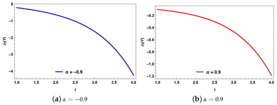
Figure 2. Plots of $J_t\left(Y_{[r:n]}\right)$ for $n=50,r=1$ for the FGM bivariate logistic distribution.

Figure 2 indicates that the values of $J_t\left(Y_{[r:n]}\right)$ are negative and its value depends on the parameter $\alpha$.

Corollary 1.

Let $(X_1,Y_1),(X_2,Y_2),\dots \dots ,(X_n,Y_n)$ be a bivariate sample of size n coming from FGM family. Then, the past extropy for concomitant of rth order statistic for $\alpha >0$ is same as past extropy for concomitant of $(n-r+1)$th order statistic with $\alpha <0$.

Proof. 

Let us denote ${\gamma }_r$ as ${\gamma }_{r,n,\alpha }$ and $J_t\left(Y_{[r:n:\alpha ]}\right)$ be the past extropy of concomitant of rth order statistic for any $\alpha$. From the definition of ${\gamma }_r$ it is clear that

$${\gamma }_{r,n,\alpha }={\gamma }_{n-2r+1,n,-\alpha }.$$

Thus, $J_t\left(Y_{[r:n:\alpha ]}\right)$ = $J_t\left(Y_{[n-2r+1:n:-\alpha ]}\right)$. Hence the corollary is attained. □

Corollary 2.

Let $(X_1,Y_1),(X_2,Y_2),\dots \dots ,(X_n,Y_n)$ be a bivariate sample of size n coming from FGM family. If n is odd, then the concomitant of median of X observations in the case of past extropy measure is same as past extropy of Y.

Proof. 

In the case, if n is odd the concomitant of median of X observations is $Y_{[\frac{n+1}{2}:n]}$. Again, we can say that ${\gamma }_r=0$ for $r=\frac{n+1}{2}$ and n is odd. Thus, $J_t\left(Y_{[\frac{n+1}{2}:n]}\right)=J_t\left(Y\right)$. The corollary is thus obtained. □

Theorem 1.

Let $Y_{[r:n]}$ be the concomitant of rth order statistic arising from FGM family, then the upper bound for past extropy of $Y_{[r:n]}$ is given by

$$J_t\left(Y_{[r:n]}\right)\le \frac{2{\gamma }_r(1+{\gamma }_r)}{F_Y\left(t\right)}E\left[U_t{f}_Y\left(F_Y^{-1}\left(U_t\right)\right)\right],$$

where $U_t\in U(0,F_Y\left(t\right))$.

Proof. 

Since $J_t\left(Y\right)\le 0$, the inequality can be obtained directly from Proposition 1. □

Theorem 2.

Let ${\kappa }_f=E\left(f_Y^2\left(Y\right)|Y<t\right)$. If $Y_{[r:n]}$ is the concomitant of rth order statistic obtained from FGM family, the lower bound for $J_t\left(Y_{[r:n]}\right)$ is

$$J_t\left(Y_{[r:n]}\right)\ge -\frac{1}{2G_{Y_{[r:n]}}^2\left(t\right)}{\kappa }_f^{\frac{1}{2}}{\left[{(1+{\gamma }_r)}^5-\frac{\left(1+{\gamma }_r-2F_Y\left(t\right){\gamma }_r\right)}{10{\gamma }_r}\right]}^{1/2}.$$

Proof. 

From Equations (7) and (10) we have

$$\begin{array}{cc}\hfill J_t\left(Y_{[r:n]}\right)& =-\frac{1}{2G_{Y_{[r:n]}}^2\left(t\right)}{\int }_0^t{f}_Y^2\left(y\right){\left[1+{\gamma }_r\left(1-2F_Y\left(y\right)\right)\right]}^{2}dy\hfill \\ \hfill & =-\frac{1}{2G_{Y_{[r:n]}}^2\left(t\right)}{\int }_0^{F_Y\left(t\right)}{f}_Y\left(F_Y^{-1}\left(u\right)\right){(1+{\gamma }_r(1-2u))}^{2}du.\hfill \end{array}$$

Use Cauchy-Schwartz inequality to get

$$\begin{array}{cc}\hfill J_t\left(Y_{[r:n]}\right)\ge & -\frac{1}{2G_{Y_{[r:n]}}^2\left(t\right)}{\left[{\int }_0^{F_Y\left(t\right)}{f}_Y^2\left(F_Y^{-1}\left(u\right)\right)du\right]}^{\frac{1}{2}}{\left[{\int }_0^{F_Y\left(t\right)}{\left(1+{\gamma }_r(1-2u)\right)}^{4}du\right]}^{\frac{1}{2}}\hfill \\ \hfill & =-\frac{1}{2G_{Y_{[r:n]}}^2\left(t\right)}{\kappa }_f^{\frac{1}{2}}{\left[{(1+{\gamma }_r)}^5-\frac{{\left(1+{\gamma }_r-2F_Y\left(t\right){\gamma }_r\right)}^5}{10{\gamma }_r}\right]}^{1/2},\hfill \end{array}$$

which completes the proof. □

3. Cumulative Past Extropy of Concomitants of Order Statistics in FGM Family

In this section, we introduce the concept of CPE for concomitant of rth order statistic. The CPE can be defined only for the rvs that have bounded range of possible values since it gives negative infinity for any rv with unbounded support. So, we limit the definition of CPE to bounded rvs. For a non-negative rv X with bounded range of values $(0,b)$, the CPE is given by

$${ℐ}_t\left(X\right)=-\frac{1}{2}{\int }_0^b{F}_X^2\left(x\right)dx.$$

Proposition 2.

Let $(X_i,Y_i)$, $i=1,2,\dots ,n$ be a bivariate random sample from FGM family. Then, the concomitant of $Y_{[r:n]}$ in the case of CPE is given by

$${ℐ}_t\left(Y_{[r:n]}\right)={\left(1+{\gamma }_r\right)}^2{ℐ}_t\left(Y\right)+{\gamma }_r\left(1+{\gamma }_r\right)E\left(\frac{U^3}{f_Y\left(F_Y^{-1}\left(U\right)\right)}\right)-\frac{{\gamma }_r^2}{2}E\left(\frac{U^4}{f_Y\left(F_Y^{-1}\left(U\right)\right)}\right),$$

(19)

where U is a rv uniformly distributed on $(0,1)$, ${ℐ}_t\left(Y\right)$ is the CPE of rv Y, and ${\gamma }_r=\alpha \frac{n-2r+1}{n+1}$.

Proof. 

For a rv Y bounded on $(0,b)$ and from the definition of ${ℐ}_t$ one may have

$$\begin{array}{cc}\hfill {ℐ}_t\left(Y_{[r:n]}\right)& =-\frac{1}{2}{\int }_0^b{G}_{Y_{[r:n]}}^2\left(y\right)dy\hfill \\ \hfill & =-\frac{1}{2}{\int }_0^b{F}_Y^2\left(y\right){\left[1+{\gamma }_r\left(1-F_Y\left(y\right)\right)\right]}^{2}dy\hfill \\ \hfill & =-\frac{1}{2}{\int }_0^b{F}_Y^2\left(y\right)\left[1+2{\gamma }_r(1-F_Y\left(y\right))+{\gamma }_r^2(1-2F_Y\left(y\right)+F_Y^2\left(y\right))\right]dy\hfill \\ \hfill & =-\frac{1}{2}\left[{(1+{\gamma }_r)}^2{\int }_0^b{F}_Y^2\left(y\right)dy-2{\gamma }_r(1+{\gamma }_r){\int }_0^b{F}_Y^3\left(y\right)+{\gamma }_r^2{\int }_0^b{F}_Y^4\left(y\right)dy\right]\hfill \\ \hfill & =-\frac{{(1+{\gamma }_r)}^2}{2}{\int }_0^1\frac{u^2}{f_Y\left(F_Y^{-1}\left(u\right)\right)}du+{\gamma }_r(1+{\gamma }_r){\int }_0^1\frac{u^3}{f_Y\left(F_Y^{-1}\left(u\right)\right)}du\hfill \\ \hfill & -\frac{{\gamma }_r^2}{2}{\int }_0^1\frac{u^4}{f_Y\left(F_Y^{-1}\left(u\right)\right)}du\hfill \\ \hfill & ={\left(1+{\gamma }_r\right)}^2{ℐ}_t\left(Y\right)+{\gamma }_r\left(1+{\gamma }_r\right)E\left(\frac{U^3}{f_Y\left(F_Y^{-1}\left(U\right)\right)}\right)-\frac{{\gamma }_r^2}{2}E\left(\frac{U^4}{f_Y\left(F_Y^{-1}\left(U\right)\right)}\right).\hfill \end{array}$$

Hence, attained the result. □

Remark 3.

In Equation (19), when $\alpha =0$ then ${\gamma }_r=0$, which implies that ${ℐ}_t\left(Y_{[r:n]}\right)={ℐ}_t\left(Y\right)$.

Remark 4.

The CPE of concomitants of the 1st and nth OS, respectively, are given by

$${ℐ}_t\left(Y_{[1:n]}\right)=\left[{\left(1+C_{n,\alpha }\right)}^2{ℐ}_t\left(Y\right)+C_{n,\alpha }\left(1+C_{n,\alpha }\right)E\left(\frac{U^3}{f_Y\left(F_Y^{-1}\left(U\right)\right)}\right)-\frac{C_{n,\alpha }^2}{2}E\left(\frac{U^4}{f_Y\left(F_Y^{-1}\left(U\right)\right)}\right)\right],$$

and

$${ℐ}_t\left(Y_{[n:n]}\right)=\left[{\left(1-C_{n,\alpha }\right)}^2{ℐ}_t\left(Y\right)-C_{n,\alpha }\left(1-C_{n,\alpha }\right)E\left(\frac{U^3}{f_Y\left(F_Y^{-1}\left(U\right)\right)}\right)-\frac{C_{n,\alpha }^2}{2}E\left(\frac{U^4}{f_Y\left(F_Y^{-1}\left(U\right)\right)}\right)\right],$$

where U∈$U(0,1)$ and $C_{n,\alpha }=\alpha \frac{n-1}{n+1}$.

Example 3.

For FGM bivariate uniform distribution with cdf given by

$$F(x,y)=\frac{x}{{\theta }_1}\frac{y}{{\theta }_2}\left[1+\alpha \left(1-\frac{x}{{\theta }_1}\right)\left(1-\frac{y}{{\theta }_2}\right)\right],$$

where $0<{\theta }_1<1$, $0<{\theta }_2<1$ and $-1\le \alpha \le 1$, the expression for ${ℐ}_t\left(Y_{[r:n]}\right)$ with parameters ${\theta }_1={\theta }_2=1$ is

$${ℐ}_t\left(Y_{[r:n]}\right)=-\frac{1}{2}\left[\frac{{\gamma }_r^2+5{\gamma }_r+10}{30}\right].$$

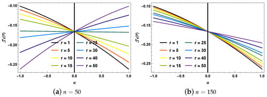
Figure 3 presents plots of ${ℐ}_t\left(Y_{[r:n]}\right)$ for sample sizes $n=50,150$ selected from FGM bivariate uniform distribution to different OS $r=1$, 5, 10, 15, 25, 30, 40, 50.

Figure 3. Plots of ${ℐ}_t\left(Y_{[r:n]}\right)$ for various selections of r based on the FGM bivariate uniform distribution.

Again, from Figure 3 it is obvious that the values of ${ℐ}_t\left(Y_{[r:n]}\right)$ are negative and the shape of the ${ℐ}_t\left(Y_{[r:n]}\right)$ depends on the sample size and the rth order statistic. Let ${\beta }_t$ be the difference between concomitant of nth order statistic and concomitant of 1st order statistic. Then,

$${\beta }_t=\frac{\alpha }{6}\left(\frac{1-n}{1+n}\right),$$

which is positive, negative or zero whenever $0<\alpha \le 1$ and $n>1$, $-1\le \alpha <0$ and $n>1$ or $\alpha =0$ and $n=1$, respectively.

Corollary 3.

For a bivariate sample from FGM family, if n is odd then the CPE for concomitant of median of X observations is same as CPE of rv Y.

Corollary 4.

For a bivariate sample obtained from FGM family, the CPE for concomitant of rth order statistic for $\alpha >0$ is same as CPE of $(n-r+1)$th order statistic for $\alpha <0$.

Theorem 3.

For a bivariate sample $(X_i,Y_i)$, $i=1,2,\dots ,n$, lower bound for ${ℐ}_t\left(Y_{[r:n]}\right)$ is given by

$${ℐ}_t\left(Y_{[r:n]}\right)\ge -\frac{1}{2}{\left[1+2{\gamma }_r^2+\frac{{\gamma }_r^4}{5}\right]}^{\frac{1}{2}}{\left[E\left(\frac{U^4}{f_Y^2\left(F_Y^{-1}\left(U\right)\right)}\right)\right]}^{\frac{1}{2}},$$

where U∈$U(0,1)$.

Proof. 

$$\begin{array}{cc}\hfill {ℐ}_t\left(Y_{[r:n]}\right)& =-\frac{1}{2}{\int }_0^b{G}_{Y_{[r:n]}}^2\left(y\right)dy\hfill \\ \hfill & =-\frac{1}{2}{\int }_0^b{F}_Y^2\left(y\right){\left[1+{\gamma }_r\left(1-F_Y\left(y\right)\right)\right]}^{2}dy\hfill \\ \hfill & =-\frac{1}{2}{\int }_0^1\frac{u^2}{f_Y\left(F_Y^{-1}\left(u\right)\right)}{\left[1+{\gamma }_r\left(1-F_Y\left(y\right)\right)\right]}^{2}du\hfill \end{array}$$

By using Cauchy-Schwartz inequality, we get

$$\begin{array}{cc}\hfill {ℐ}_t\left(Y_{[r:n]}\right)\ge & -\frac{1}{2}{\left[{\int }_0^1{\left(1+{\gamma }_r(1-u)\right)}^4\right]}^{\frac{1}{2}}{\left[{\int }_0^1\frac{u^4}{f_Y^2\left(F_Y^{-1}\left(u\right)\right)}\right]}^{\frac{1}{2}}\hfill \\ \hfill & =-\frac{1}{2}{\left[1+2{\gamma }_r^2+\frac{{\gamma }_r^4}{5}\right]}^{\frac{1}{2}}{\left[E\left(\frac{U^4}{f_Y^2\left(F_Y^{-1}\left(U\right)\right)}\right)\right]}^{\frac{1}{2}}.\hfill \end{array}$$

Hence the proof is attained. □

4. Dynamic Survival Past Extropy for Concomitants of Order Statistics in FGM Family

Here, we derive the expression for measures of DSPE for concomitant of rth order statistic.

Proposition 3.

Let $(X_1,Y_1),(X_2,Y_2),\dots \dots ,(X_n,Y_n)$ be a bivariate sample of size n from FGM family. The concomitant of rth order statistic for DSPE measure, $J_{DS{P}_t}\left(Y_{[r:n]}\right)$ is

$$\begin{array}{cc}\hfill J_{DS{P}_t}\left(Y_{[r:n]}\right)& ={\left(\frac{1}{1+{\gamma }_r(1-F_Y\left(t\right))}\right)}^2[{\left(1+{\gamma }_r\right)}^2{J}_{DS{P}_t}\left(Y\right)\hfill \\ \hfill & +\frac{{\gamma }_r\left(1+{\gamma }_r\right)}{F_Y\left(t\right)}E\left(\frac{U_t^3}{f_Y\left(F_Y^{-1}\left(U_t\right)\right)}\right)-\frac{{\gamma }_r^2}{2F_Y\left(t\right)}E\left(\frac{U_t^4}{f_Y\left(F_Y^{-1}\left(U_t\right)\right)}\right)],\hfill \end{array}$$

(20)

where $J_{DS{P}_t}\left(Y\right)$ is DSPE of rv Y, $U_t$∈$U(0,F_Y\left(t\right))$ and ${\gamma }_r=\alpha \frac{n-2r+1}{n+1}$.

Proof. 

To prove the proposition, from Equation (3) we have

$$J_{DS{P}_t}\left(Y_{[r:n]}\right)=-\frac{1}{2}{\int }_0^t\frac{G_{Y_{[r:n]}}^2\left(y\right)}{G_{Y_{[r:n]}}^2\left(t\right)}dy,$$

where is $G_{Y_{[r:n]}}^2\left(y\right)$ defined in Equation (8). Then,

$$\begin{array}{cc}\hfill J_{DS{P}_t}\left(Y_{[r:n]}\right)& =-\frac{1}{2}{\int }_0^t\frac{F_Y^2\left(y\right){\left[1+{\gamma }_r\left(1-F_Y\left(y\right)\right)\right]}^2}{G_{Y_{[r:n]}}^2\left(t\right)}dy\hfill \\ \hfill & =-\frac{1}{2}{\int }_0^t\frac{F_Y^2\left(y\right)[1+2{\gamma }_r(1-F_Y\left(y\right))+{\gamma }_r^2(1-2F_Y\left(y\right)+F_Y^2\left(y\right))]}{G_{Y_{[r:n]}}^2\left(t\right)}dy.\hfill \end{array}$$

Rearranging, we get

$$\begin{array}{cc}\hfill J_{DS{P}_t}\left(Y_{[r:n]}\right)& =-\frac{1}{2G_{Y_{[r:n]}}^2\left(t\right)}\left[{(1+{\gamma }_r)}^2{\int }_0^t{F}_Y^2\left(y\right)dy-2{\gamma }_r(1+{\gamma }_r){\int }_0^t{F}_Y^3\left(y\right)+{\gamma }_r^2{\int }_0^t{F}_Y^4\left(y\right)dy\right].\hfill \end{array}$$

Using Equation (8), this equation will be

$$\begin{array}{cc}\hfill J_{DS{P}_t}\left(Y_{[r:n]}\right)=& -\frac{1}{2}{\left(\frac{1}{1+{\gamma }_r(1-F_Y\left(t\right))}\right)}^2[\frac{{(1+{\gamma }_r)}^2}{F_Y^2\left(t\right)}{\int }_0^t{F}_Y^2\left(y\right)dy\hfill \\ \hfill & -\frac{2{\gamma }_r(1+{\gamma }_r)}{F_Y^2\left(t\right)}{\int }_0^t{F}_Y^3\left(y\right)dy+\frac{{\gamma }_r^2}{F_Y^2\left(t\right)}{\int }_0^t{F}_Y^4\left(y\right)dy]\hfill \\ \hfill =& {\left(\frac{1}{1+{\gamma }_r(1-F_Y\left(t\right))}\right)}^2[-\frac{{(1+{\gamma }_r)}^2}{2F_Y^2\left(t\right)}{\int }_0^{F_Y\left(t\right)}\frac{u^2}{f_Y\left(F_Y^{-1}\left(u\right)\right)}du\hfill \\ \hfill & +\frac{{\gamma }_r(1+{\gamma }_r)}{F_Y^2\left(t\right)}{\int }_0^{F_Y\left(t\right)}\frac{u^3}{f_Y\left(F_Y^{-1}\left(u\right)\right)}du-\frac{{\gamma }_r^2}{2F_Y^2\left(t\right)}{\int }_0^{F_Y\left(t\right)}\frac{u^4}{f_Y\left(F_Y^{-1}\left(u\right)\right)}du]\hfill \\ \hfill =& {\left(\frac{1}{1+{\gamma }_r(1-F_Y\left(t\right))}\right)}^2[{\left(1+{\gamma }_r\right)}^2{J}_{DS{P}_t}\left(Y\right)\hfill \\ \hfill & +\frac{{\gamma }_r(1+{\gamma }_r)}{F_Y^2\left(t\right)}{\int }_0^{F_Y\left(t\right)}\frac{u^3}{f_Y\left(F_Y^{-1}\left(u\right)\right)}du-\frac{{\gamma }_r^2}{2F_Y^2\left(t\right)}{\int }_0^{F_Y\left(t\right)}\frac{u^4}{f_Y\left(F_Y^{-1}\left(u\right)\right)}du]\hfill \\ \hfill =& {\left(\frac{1}{1+{\gamma }_r(1-F_Y\left(t\right))}\right)}^2[{\left(1+{\gamma }_r\right)}^2{J}_{DS{P}_t}\left(Y\right)\hfill \\ \hfill & +\frac{{\gamma }_r\left(1+{\gamma }_r\right)}{F_Y\left(t\right)}E\left(\frac{U_t^3}{f_Y\left(F_Y^{-1}\left(U_t\right)\right)}\right)-\frac{{\gamma }_r^2}{2F_Y\left(t\right)}E\left(\frac{U_t^4}{f_Y\left(F_Y^{-1}\left(U_t\right)\right)}\right)].\hfill \end{array}$$

Hence, the result is attained. □

Remark 5.

When $\alpha =0$ in Equation (20), then ${\gamma }_r=0$, which implies $J_{DS{P}_t}\left(Y_{[r:n]}\right)=J_{DS{P}_t}\left(Y\right)$.

Remark 6.

The concomitants of 1st and nth OS of a random sample of size n are obtained using $r=1,r=n$. Then, the DSPE measure for concomitants of the corresponding OS, respectively are

$$\begin{array}{cc}\hfill J_{DS{P}_t}\left(Y_{[1:n]}\right)& ={\left(\frac{1}{1+C_{n,\alpha }(1-F_Y\left(t\right))}\right)}^2\left[{\left(1+C_{n,\alpha }\right)}^2{J}_{DS{P}_t}\left(Y\right)\right.\hfill \\ \hfill & \left.+\frac{C_{n,\alpha }\left(1+C_{n,\alpha }\right)}{F_Y\left(t\right)}E\left(\frac{U_t^3}{f_Y\left(F_Y^{-1}\left(U_t\right)\right)}\right)-\frac{C_{n,\alpha }^2}{2F_Y\left(t\right)}E\left(\frac{U_t^4}{f_Y\left(F_Y^{-1}\left(U_t\right)\right)}\right)\right],\hfill \end{array}$$

(21)

and

$$\begin{array}{cc}\hfill J_{DS{P}_t}\left(Y_{[n:n]}\right)& ={\left(\frac{1}{1-C_{n,\alpha }(1-F_Y\left(t\right))}\right)}^2\left[{\left(1-C_{n,\alpha }\right)}^2{J}_{DS{P}_t}\left(Y\right)\right.\hfill \\ \hfill & \left.-\frac{C_{n,\alpha }\left(1-C_{n,\alpha }\right)}{F_Y\left(t\right)}E\left(\frac{U_t^3}{f_Y\left(F_Y^{-1}\left(U_t\right)\right)}\right)-\frac{C_{n,\alpha }^2}{2F_Y\left(t\right)}E\left(\frac{U_t^4}{f_Y\left(F_Y^{-1}\left(U_t\right)\right)}\right)\right],\hfill \end{array}$$

(22)

where $U_t$ is a rv distributed uniformly on $(0,F_Y\left(t\right))$ and $C_{n,\alpha }=\alpha \frac{n-1}{n+1}$.

Example 4.

If $(X,Y)$ is a bivariate sample from FGM bivariate exponential distribution with the cdf given in Equation (13), then

$$J_{DS{P}_t}\left(Y_{[r:n]}\right)=\frac{6e^{\frac{2t}{{\theta }_2}}\left({\theta }_2-4e^{\frac{t}{{\theta }_2}}{\theta }_2+e^{\frac{2t}{{\theta }_2}}(3{\theta }_2-2t)\right)-{\left(-1+e^{\frac{t}{{\theta }_2}}\right)}^3{\theta }_2{\gamma }_r\left(3{\gamma }_r+e^{\frac{t}{{\theta }_2}}(8+{\gamma }_r)\right)}{24{\left(-1+e^{\frac{t}{{\theta }_2}}\right)}^2{\left(e^{\frac{t}{{\theta }_2}}+{\gamma }_r\right)}^2}.$$

(23)

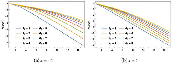
Figure 4 presents some plots of $J_{DSPt}\left(Y_{[r:n]}\right)$ for a sample of size $n=50,r=1$ selected from FGM bivariate exponential distribution with $\alpha =-1,1$.

Figure 4. Plots of $J_{DSPt}\left(Y_{[r:n]}\right)$ for $\alpha =-1,1$ based on the FGM bivariate exponential distribution.

From Figure 4 it is obvious that the values of $J_{DSPt}\left(Y_{[r:n]}\right)$ are negative and its shape depends on the parameter values $\alpha =-1,1$. Let ${\delta }_t$ be the difference between DSPE of concomitants of nth and 1st OS. It is given by

$$\begin{array}{c}\hfill {\delta }_t=\frac{e^{\frac{t}{{\theta }_2}}(-1+n^2)\alpha }{6{\left(-1+e^{\frac{t}{{\theta }_2}}\right)}^2{\left(e^{\frac{t}{{\theta }_2}}(1+n)+(-1+n)\alpha \right)}^2{\left(e^{\frac{t}{{\theta }_2}}(1+n)+(1-n)\alpha \right)}^2}(4e^{\frac{5t}{{\theta }_2}}{(1+n)}^2{\theta }_2\\ \hfill -{(1+n)}^2{\alpha }^2{\theta }_2+4e^{\frac{t}{{\theta }_2}}{(-1+n)}^2{\alpha }^2{\theta }_2+4e^{\frac{3t}{{\theta }_2}}\left(-3{(1+n)}^2+{(-1+n)}^2{\alpha }^2\right){\theta }_2\\ \hfill -2e^{\frac{2t}{{\theta }_2}}\left(-{(1+n)}^2+3{(-1+n)}^2{\alpha }^2\right){\theta }_2-e^{\frac{4t}{{\theta }_2}}\left(12{(1+n)}^{2}t+\left(-6{(1+n)}^2+{(-1+n)}^2{\alpha }^2\right){\theta }_2\right)).\end{array}$$

Hence, ${\delta }_t$ is positive when $0<\alpha \le 1$ and $n>1$, is negative when $-1\le \alpha <0$ and $n>1$, is zero when $\alpha =0$ and $n=1$.

Example 5.

Let the bivariate sample is selected from FGM bivariate logistic distribution with cdf given in Equation (16), the DSPE of $Y_{[r:n]}$ is given by

$$\begin{array}{c}\hfill J_{DS{P}_t}\left(Y_{[r:n]}\right)=-\frac{1}{24{\left(1+e^t\right)}^3{\left(1+\left(1-\frac{1}{1+e^{-t}}\right){\gamma }_r\right)}^2}\left({\left(1+e^{-t}\right)}^2{\left(-6(1+e^{-t})\right)}^2\right(-1+log\left(4\right)\\ \hfill +e^t(1+log\left(4\right))-2(1+e^t)log(1+e^t))+(-1+e^t){\gamma }_r\left(3+{\gamma }_r+4e^t(3+{\gamma }_r)+e^{2t}(9+{\gamma }_r)\right)).\end{array}$$

Next,

$$\begin{array}{c}\hfill {\delta }_t=\frac{e^{-2t}(1+e^t)(-1+n^2)\alpha }{\left(12{\left(1+n+e^t(1+n)+(-1+n)\alpha \right)}^2{\left(1+n+e^t(1+n)+(1-n)\alpha \right)}^2\right)}\left[\right(-15\\ \hfill +9e^{4t}{\left(1+n\right)}^2-{\alpha }^2+24log2+n\left(-30-15n+2{\alpha }^2-n{\alpha }^2+24(2+n)log2\right)+e^{3t}(24-2{\alpha }^2\\ \hfill +24log2+2n\left(24+12n+2{\alpha }^2-n{\alpha }^2+12(2+n)log2\right))+3e^{2t}(2+{\alpha }^2\\ \hfill +24log2+n\left(4+2n-2{\alpha }^2+n{\alpha }^2+24(2+n)log2\right))+24e^t{(1+n)}^2\\ \hfill (-1+log8)-24{(1+e^t)}^3{(1+n)}^{2}log(1+e^t)\left)\right]\end{array}$$

is positive for $n>1$ when $0<\alpha \le 1$, negative in the range $-1\le \alpha <0$ for $n>1$ and zero when $n=1$ with $\alpha =0$.

Corollary 5.

For a bivariate sample obtained from FGM family, the DSPE for concomitant of rth order statistic for $\alpha >0$ is same as DSPE of $(n-r+1)$th order statistic for $\alpha <0$.

Proof. 

The proof is similar to the proof of Corollary (1). Hence, $J_{DS{P}_t{}_{\left(\alpha \right)}}\left(Y_{[r:n]}\right)=J_{DS{P}_t{}_{(-\alpha )}}$$\left(Y_{[n-r+1:n]}\right)$. □

Corollary 6.

For a bivariate sample from FGM family, if n is odd then the $DSPE$ for concomitant of median of X observations is same as DSPE of rv Y.

Proof. 

The proof is similar to the proof of Corollary (2) and hence omitted. □

Theorem 4.

The upper bound for DSPE of $Y_{[r:n]}$ is given by

$$J_{DS{P}_t}\left(Y_{[r:n]}\right)\le \frac{{\gamma }_r(1+{\gamma }_r)}{F_Y\left(t\right)}E\left[U_t\left(f_Y\left(F_Y^{-1}\left(U_t\right)\right)\right)\right],$$

where $U_t\in U(0,F_Y\left(t\right))$ and $Y_{[r:n]}$ is the concomitant of rth order statistic arising from FGM family.

Proof. 

Since the DSPE ≤ 0, by using Proposition (3) we can obtain the inequality straightly. Hence, the theorem is attained. □

Theorem 5.

If $Y_{[r:n]}$ denotes the concomitant of rth order statistic arising from FGM family, then the lower bound of DSPE is

$$\begin{array}{c}\hfill J_{DS{P}_t}\left(Y_{[r:n]}\right)\ge -\frac{1}{2}{\left(\frac{1}{1+{\gamma }_r(1-F_Y\left(t\right))}\right)}^2{\left[\frac{1}{F_Y^2\left(t\right)}\frac{{(1+{\gamma }_r)}^5-{(-1+(-1+F_Y\left(t\right)){\gamma }_r)}^5}{5{\gamma }_r}\right]}^{\frac{1}{2}}\\ \hfill {\left[\frac{1}{F_Y\left(t\right)}E\left(\frac{U_t^4}{f_Y^2\left(F_Y^{-1}\left(U_t\right)\right)}\right)\right]}^{\frac{1}{2}},\end{array}$$

where $U_t\in U(0,F_Y\left(t\right))$.

Proof. 

Based on Equation (3), we have

$$\begin{array}{cc}\hfill J_{DS{P}_t}\left(Y_{[r:n]}\right)& =-\frac{1}{2}{\int }_0^t\frac{G_{Y_{[r:n]}}^2\left(y\right)}{G_{Y_{[r:n]}}^2\left(t\right)}dy\hfill \\ \hfill & =-\frac{1}{2}{\left(\frac{1}{F_Y^2\left(t\right)(1+{\gamma }_r(1-F_Y\left(t\right)))}\right)}^2{\int }_0^t{F}_Y^2\left(y\right){\left[1+{\gamma }_r\left(1-F_Y\left(y\right)\right)\right]}^{2}dy\hfill \\ \hfill & =-\frac{1}{2}{\left(\frac{1}{F_Y^2\left(t\right)(1+{\gamma }_r(1-F_Y\left(t\right)))}\right)}^2{\int }_0^{F_Y\left(t\right)}\frac{u^2{\left((1+{\gamma }_r(1-u)\right)}^2}{f_Y\left(F_Y^{-1}\left(u\right)\right)}du.\hfill \end{array}$$

Using Cauchy-Schwartz inequality to get

$$\begin{array}{cc}\hfill J_{DS{P}_t}\left(Y_{[r:n]}\right)\ge & -\frac{1}{2}{\left(\frac{1}{(1+{\gamma }_r(1-F_Y\left(t\right)))}\right)}^2{\left[\frac{1}{F_Y^2\left(t\right)}{\int }_0^{F_Y\left(t\right)}\frac{u^4}{f_Y^2\left(F_Y^{-1}\left(u\right)\right)}\right]}^{\frac{1}{2}}\hfill \\ & {\left[\frac{1}{F_Y^2\left(t\right)}{\int }_0^{F_Y\left(t\right)}{\left(1+{\gamma }_r(1-u)\right)}^4\right]}^{\frac{1}{2}}\hfill \\ \hfill & =-\frac{1}{2}{\left(\frac{1}{(1+{\gamma }_r(1-F_Y\left(t\right)))}\right)}^2{\left[\frac{1}{F_Y\left(t\right)}E\left(\frac{U_t^4}{f_Y^2\left(F_Y^{-1}\left(U_t\right)\right)}\right)\right]}^{\frac{1}{2}}\hfill \\ & {\left[\frac{1}{F_Y^2\left(t\right)}\frac{{(1+{\gamma }_r)}^5-{(-1+(-1+F_Y\left(t\right)){\gamma }_r)}^5}{5{\gamma }_r}\right]}^{\frac{1}{2}}.\hfill \end{array}$$

Hence, the theorem is proved. □

5. Estimation of CPE for Concomitant of rth Order Statistic

Here, the problem of estimating the CPE of rth order statistic using the empirical CPE is considered. Let $(X_i,Y_i)$ be a sequence obtained from the FGM family. Using Equation (19), the empirical CPE of $Y_{[r:n]}$ is derived as

$$\begin{array}{cc}\hfill \widehat{ℐ}\left(Y_{[r:n]}\right)& =-\frac{1}{2}\left[{(1+{\gamma }_r)}^2{\int }_0^{\infty }{\widehat{F}}_Y^2\left(y\right)dy-2{\gamma }_r(1+{\gamma }_r){\int }_0^{\infty }{\widehat{F}}_Y^3\left(y\right)dy+{\gamma }_r^2{\int }_0^{\infty }{\widehat{F}}_Y^4\left(y\right)dy\right]\hfill \\ \hfill & =-\frac{1}{2}[{(1+{\gamma }_r)}^2\sum _{i=1}^{n-1}{\int }_{Z_i}^{Z_{i+1}}{\widehat{F}}_Y^2\left(y\right)dy-2{\gamma }_r(1+{\gamma }_r)\sum _{i=1}^{n-1}{\int }_{Z_i}^{Z_{i+1}}{\widehat{F}}_Y^3\left(y\right)dy\hfill \\ \hfill & +{\gamma }_r^2\sum _{i=1}^{n-1}{\int }_{Z_i}^{Z_{i+1}}{\widehat{F}}_Y^4\left(y\right)dy]\hfill \\ \hfill & =-\frac{1}{2}\left[{(1+{\gamma }_r)}^2\sum _{i=1}^{n-1}{U}_i{\left(\frac{i}{n}\right)}^2-2{\gamma }_r(1+{\gamma }_r)\sum _{i=1}^{n-1}{U}_i{\left(\frac{i}{n}\right)}^3+{\gamma }_r^2\sum _{i=1}^{n-1}{U}_i{\left(\frac{i}{n}\right)}^4\right]\hfill \\ \hfill & =-\frac{1}{2}\sum _{i=1}^{n-1}{U}_i{\left(\frac{i}{n}\right)}^2\left[{(1+{\gamma }_r)}^2-2{\gamma }_r(1+{\gamma }_r)\left(\frac{i}{n}\right)+{\gamma }_r^2{\left(\frac{i}{n}\right)}^2\right]\hfill \\ \hfill & =-\frac{1}{2}\sum _{i=1}^{n-1}{U}_i{\left(\frac{i}{n}\right)}^2{\left[1+{\gamma }_r\left(1-\frac{i}{n}\right)\right]}^2,\hfill \end{array}$$

(24)

where $U_i=Z_{i+1}-Z_i$, $i=1,2,\dots ,n-1$ are the sample spacings based on rv Y.

Example 6.

For FGM bivariate uniform distribution, the spacings $U_i$ are independent beta distributed with parameters 1 and n. Then,

$$E\left(\widehat{ℐ}\left(Y_{[r:n]}\right)\right)=-\frac{1}{2(n+1)}\sum _{i=1}^{n-1}{\left(\frac{i}{n}\right)}^2{\left(1+{\gamma }_r\left(1-\frac{i}{n}\right)\right)}^2,$$

(25)

and

$$Var\left(\widehat{ℐ}\left(Y_{[r:n]}\right)\right)=\frac{n}{4{(n+1)}^2(n+2)}\sum _{i=1}^{n-1}{\left(\frac{i}{n}\right)}^4{\left(1+{\gamma }_r\left(1-\frac{i}{n}\right)\right)}^4.$$

(26)

We figured the values of $E\left(\widehat{ℐ}\left(Y_{[2:n]}\right)\right)$ and $Var\left(\widehat{ℐ}\left(Y_{[2:n]}\right)\right)$ for different sample sizes $n=5,15,25,50$ for $\alpha =-1,-0.5,0.5,1$ in the case of FGM bivariate uniform distribution, and the results are given in Table 1 and Table 2.

Table 1. Values of $E\left(\widehat{ℐ}\left(Y_{[2:n]}\right)\right)$ for FGM bivariate uniform distribution with ${\theta }_1$ = ${\theta }_2$ = 1.

n	$\mathit{\alpha }=-1$	$\mathit{\alpha }=-0.5$	$\mathit{\alpha }=0.5$	$\mathit{\alpha }=1$
5	−0.0793	−0.0892	−0.1114	−0.1237
15	−0.0914	−0.1140	−0.1549	−0.2080
25	−0.0945	−0.1197	−0.1723	−0.2299
50	−0.0971	−0.1243	−0.1816	−0.2476

Table 2. Values of $Var\left(\widehat{ℐ}\left(Y_{[2:n]}\right)\right)$ for FGM bivariate uniform distribution with ${\theta }_1$ = ${\theta }_2$ = 1.

n	$\mathit{\alpha }=-1$	$\mathit{\alpha }=-0.5$	$\mathit{\alpha }=0.5$	$\mathit{\alpha }=1$
5	0.0019	0.0023	0.0033	0.0040
15	0.0012	0.0016	0.0029	0.0039
25	0.0008	0.0011	0.0021	0.0029
50	0.0004	0.0006	0.0012	0.0017

The following properties can be attained from Table 1 and Table 2:

• For a fixed value of n, the values of $E\left(\widehat{ℐ}\left(Y_{[2:n]}\right)\right)$ are decreasing as the values of $\alpha$ increases, whereas the values of $Var\left(\widehat{ℐ}\left(Y_{[2:n]}\right)\right)$ are increasing with $\alpha$.
• For a fixed $\alpha$, both the values of $E\left(\widehat{ℐ}\left(Y_{[2:n]}\right)\right)$ and $Var\left(\widehat{ℐ}\left(Y_{[2:n]}\right)\right)$ are decreasing with the increasing value of n.
• As n tends to infinity, the value of $Var\left(\widehat{ℐ}\left(Y_{[2:n]}\right)\right)$ tends to zero.

6. Simulation

A Monte Carlo simulation study is conducted to validate the above proposed empirical estimator of CPE. Data is obtained through random generation following the FGM bivariate uniform distribution with parameter values of ${\theta }_1$ and ${\theta }_2$ set to 1. The study involves varying values of $\alpha$ to analyze and explore different scenarios using the generated data. Empirical CPE, theoretical CPE, bias, and mean squared error (MSE) for $Y_{[r:n]}$ are calculated for different values of sample size n and specific $\alpha$. These computations are performed at various OS, allowing for an analysis between empirical and theoretical values while also assessing bias and accuracy for different scenarios, which are showed in Table 3 and Figure 5.

Table 3. Theoretical value, Estimated value, bias and MSE of CPE of $Y_{[r:n]}$ for different values of r, $\alpha$ and n.

r	$\mathit{\alpha }$	n	${\mathit{ℐ}}_{\mathit{t}}\left({\mathit{Y}}_{[\mathit{r}:\mathit{n}]}\right)$	$\widehat{\mathit{ℐ}}\left({\mathit{Y}}_{[\mathit{r}:\mathit{n}]}\right)$	Bias	MSE
2	0.2	50	−0.1825	−0.1747	0.0078	0.0005
	0.2	100	−0.1832	−0.1782	0.0050	0.0002
	0.2	200	−0.1836	−0.1815	0.0020	0.0001
	0.5	50	−0.2086	−0.1991	0.0094	0.0005
	0.5	100	−0.2105	−0.2064	0.0040	0.0002
	0.5	200	−0.2115	−0.2092	0.0022	0.0001
	0.8	50	−0.2371	−0.2280	0.0091	0.0005
	0.8	100	−0.2405	−0.2360	0.0044	0.0003
	0.8	200	−0.2422	−0.2399	0.0023	0.0001
4	0.2	50	−0.1811	−0.1718	0.0093	0.0005
	0.2	100	−0.1825	−0.1788	0.0037	0.0002
	0.2	200	−0.1832	−0.1807	0.0025	0.0001
	0.5	50	−0.2047	−0.1958	0.0089	0.0005
	0.5	100	−0.2085	−0.2046	0.0039	0.0002
	0.5	200	−0.2105	−0.2081	0.0023	0.0001
	0.8	50	−0.2304	−0.2209	0.0095	0.0005
	0.8	100	−0.2370	−0.2321	0.0049	0.0003
	0.8	200	−0.2405	−0.2378	0.0026	0.0001
10	0.2	50	−0.1770	−0.1678	0.0092	0.0004
	0.2	100	−0.1804	−0.1763	0.0041	0.0002
	0.2	200	−0.1822	−0.1801	0.0020	0.0001
	0.5	50	−0.1935	−0.1851	0.0083	0.0005
	0.5	100	−0.2027	−0.1982	0.0045	0.0002
	0.5	200	−0.2075	−0.2051	0.0024	0.0001
	0.8	50	−0.2111	−0.2034	0.0076	0.0005
	0.8	100	−0.2269	−0.2227	0.0042	0.0002
	0.8	200	−0.2353	−0.2334	0.0018	0.0001

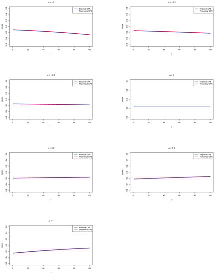
Figure 5. CPE of $Y_{[r:n]}$ (red) and empirical CPE of $Y_{[r:n]}$ (blue) in the case of FGM bivariate uniform distribution for $n=100$.

From Table 3, it is clear that as the sample size n increases, both the bias and MSE decrease, and in the case of the MSE, it approaches zero. This trend indicates that the estimator is performing well in this scenario. The decreasing bias implies that the estimator tends to be more accurate as the sample size becomes larger. The diminishing MSE suggests that the estimator’s predictions are closer to the true values with increasing sample size, signifying improved estimation accuracy and efficiency.

The following conclusions can be obtained from the Figure 5. They are,

• In all the cases discussed in the figure, both ${ℐ}_t\left(Y_{[r:n]}\right)$ and $\widehat{ℐ}\left(Y_{[r:n]}\right)$ behaves alike. Both the values are almost similar for various values of OS.
• For $\alpha <0$, both the theoretical and empirical CPE of $Y_{[r:n]}$ show a decreasing trend as the value of r increases.
• On the other hand, for $\alpha >0$, both the functions ${ℐ}_t\left(Y_{[r:n]}\right)$ and $\widehat{ℐ}\left(Y_{[r:n]}\right)$ exhibit an increasing pattern as r falls within this range.

7. Conclusions and Future Works

In this work, we have considered the properties of past extropy, CPE, DSPE for concomitant of rth order statistic in FGM family. Several properties and bounds related to the above three measures for COS are developed. Estimation of CPE has been done using empirical estimation. The validity of the proposed estimators has been backed through numerical calculations on FGM uniform distribution and simulation study. From the simulation study, it can be concluded that the empirical CPE of $Y_{[r:n]}$ exhibits a behavior similar to the theoretical CPE of $Y_{[r:n]}$. When $\alpha <0$, as r increases, both the theoretical and empirical CPE of $Y_{[r:n]}$ decrease, whereas for $\alpha >0$, both the theoretical and empirical CPE of $Y_{[r:n]}$ increase with decreasing r in this range. The proposed estimator is considered good based on its MSE performance. This suggests that the estimator is capable of providing reliable and satisfactory estimates, making it a favorable choice for the given scenario.

COS play a crucial role in diverse selection processes. One significant application of COS lies in sampling procedures, including RSS, double sampling, and others. Investigating the information content of different information measures using these sampling designs in terms of COS could be a valuable addition to existing literature. To conduct such a study, COS can be derived from various bivariate families like FGM and Sarmanov.

References

- David, H.A. Concomitants of order statistics. Bull. Int. Stat. Inst. 1973, 45, 295–300. [Google Scholar]
- David, H.A.; Nagaraja, H.N. Concomitants of order statistics. In Handbook of Statistics; Balakrishnan, N., Rao, C.R., Eds.; Elsevier: Amsterdam, The Netherlands, 1998; pp. 487–513. [Google Scholar]
- Morgenstern, D. Einfache beispiele zweidimensionaler verteilungen. Mitteilungsblatt Math. Stat. 1956, 8, 234–235. [Google Scholar]
- Bairamov, I.; Kotz, S.; Bekci, M. New generalized Farlie-Gumbel-Morgenstern distributions and concomitants of order statistics. J. Appl. Stat. 2001, 28, 521–536. [Google Scholar] [CrossRef]
- Susam, S.O. A multi-parameter Generalized Farlie-Gumbel-Morgenstern bivariate copula family via Bernstein polynomial. Hacet. J. Math. Stat. 2022, 51, 618–631. [Google Scholar] [CrossRef]
- Shannon, C.E. A mathematical theory of communication. Bell Syst. Tech. J. 1948, 27, 379–432. [Google Scholar] [CrossRef]
- Baratpour, S.; Ahmadi, J.; Arghami, N.R. Some characterizations based on entropy of order statistics and record values. Commun. Stat.-Theory Methods 2007, 36, 47–57. [Google Scholar] [CrossRef]
- Al-Omari, A.I. A new measure of sample entropy of continuous random variable. J. Stat. Theory Pract. 2015, 10, 721–735. [Google Scholar] [CrossRef]
- Al-Omari, A.I. Estimation of entropy using random sampling. J. Comput. Appl. Math. 2014, 261, 95–102. [Google Scholar] [CrossRef]
- Song, K.S. A mathematical theory of communication. J. Stat. Plan. Inference 2001, 93, 51–69. [Google Scholar] [CrossRef]
- Frank, L.; Sanfilippo, G.; Agro, G. Extropy: Complementary dual of entropy. Stat. Sci. 2015, 30, 40–58. [Google Scholar]
- Martinas, K.; Frankowicz, M. Extropy-reformulation of the Entropy Principle. Period. Polytech. Chem. Eng. 2000, 44, 29–38. [Google Scholar]
- Becerra, A.; de la Rosa, J.I.; Gonzalez, E.; Pedroza, A.D.; Escalante, N.I. Training deep neural networks with non-uniform frame-level cost function for automatic speech recognition. Multimed. Tools Appl. 2018, 77, 27231–27267. [Google Scholar] [CrossRef]
- Qiu, G. Extropy of order statistics and record values. Stat. Probab. Lett. 2017, 120, 52–60. [Google Scholar] [CrossRef]
- Qiu, G.; Wang, L.; Wang, X. On extropy properties of mixed systems. Probab. Eng. Inf. Sci. 2019, 33, 471–486. [Google Scholar] [CrossRef]
- Gupta, N.; Chaudhary, S.K. On general weighted extropy of ranked set sampling. Commun. Stat.-Theory Methods 2023. [Google Scholar] [CrossRef]
- Di Crescenzo, A.; Longobardi, M. Entropy-based measure of uncertainity in past lifetime distributions. J. Appl. Probab. 2002, 39, 434–440. [Google Scholar] [CrossRef]
- Krishnan, A.S.; Sunoj, S.M.; Nair, N.U. Some reliability properties of extropy for residual and past lifetime random variables. J. Korean Stat. Soc. 2020, 49, 457–474. [Google Scholar] [CrossRef]
- Kamari, O.; Buono, F. On extropy of past lifetime distribution. Ric. Mat. 2021, 70, 505–515. [Google Scholar] [CrossRef]
- Vaselabadi, N.M.; Tahmasebi, S.; Kazemi, M.R.; Buono, F. Results on varextropy measure of random variables. Entropy 2021, 23, 356. [Google Scholar] [CrossRef]
- Irshad, M.R.; Maya, R.; Archana, K.; Tahmasebi, S. On Past Extropy and Negative Cumulative Extropy Properties of Ranked Set Sampling and Maximum Ranked Set Sampling with Unequal Samples. Stat. Optim. Inf. Comput. 2023, 11, 740–754. [Google Scholar]
- Jose, J.; Abdul Sathar, E.I. Extropy for past life based on classical records. Extropy Past Life Based Class. Rec. 2021, 22, 27–46. [Google Scholar] [CrossRef]
- Sathar, E.A.; Nair, R.D. On dynamic weighted extropy. J. Comput. Appl. Math. 2021, 393, 113507. [Google Scholar] [CrossRef]
- Abdul Sathar, E.I.; Nair, R.D. On dynamic survival extropy. Commun. Stat.-Theory Methods 2020, 50, 1295–1313. [Google Scholar] [CrossRef]
- Pakdaman, Z.; Hashempour, M. On dynamic survival past extropy properties. J. Stat. Res. Iran 2019, 16, 229–244. [Google Scholar]
- Abo-Eleneen, Z.A.; Nagaraja, H.N. Fisher information in an order statistic and its concomitant. Ann. Inst. Stat. Math. 2002, 54, 667–680. [Google Scholar] [CrossRef]
- Tahmasebi, S.; Behboodian, J. Information properties for concomitants of order statistics in Farlie–Gumbel–Morgenstern (FGM) Family. Commun. Stat.-Theory Methods 2012, 41, 1954–1968. [Google Scholar] [CrossRef]
- Almaspoor, Z.; Jafari, A.A.; Tahmasebi, S. Measures of extropy for concomitants of generalized order statistics in Morgenstern Family. J. Stat. Theory Appl. 2022, 21, 1–20. [Google Scholar] [CrossRef]
- Mohamed, M.S.; Abdulrahman, A.T.; Almaspoor, Z.; Yusuf, M. Ordered variables and their concomitants under extropy via COVID-19 data application. Complexity 2021, 2021, 6491817. [Google Scholar] [CrossRef]
- Hussiney, I.A.; Shyam, A.H. The extropy of concomitants of generalized order statistics from Huang–Kotz–Morgenstern bivariate distribution. Hindawi J. Math. 2022, 2022, 6385998. [Google Scholar] [CrossRef]
- Mohie EL-Din, M.M.; Amein, M.M.; Ali, N.S.A.; Mohamed, M.S. Residual and past entropy for concomitants of ordered random variables of Morgenstern Family. Hindawi J. Math. 2015, 2015, 159710. [Google Scholar] [CrossRef]
- Johnson, N.L.; Kotz, S. On some generalized Farlie–Gumbel–Morgenstern distributions. Commun. Stat.-Theory Methods 1975, 4, 415–427. [Google Scholar]
- Scaria, J.; Nair, U. On concomitants of order statistics from Morgenstern family. Biom. J. 1999, 41, 483–489. [Google Scholar] [CrossRef]
Disclaimer/Publisher’s Note: The statements, opinions and data contained in all publications are solely those of the individual author(s) and contributor(s) and not of MDPI and/or the editor(s). MDPI and/or the editor(s) disclaim responsibility for any injury to people or property resulting from any ideas, methods, instructions or products referred to in the content. |
© 2023 by the authors. Licensee MDPI, Basel, Switzerland. This article is an open access article distributed under the terms and conditions of the Creative Commons Attribution (CC BY) license (https://creativecommons.org/licenses/by/4.0/).