Article

A Method for Extrapolating Continuous Functions by Generating New Training Samples for Feedforward Artificial Neural Networks

Faculty of Mathematics and Informatics, University of Plovdiv Paisii Hilendarski, 236 Bulgaria Blvd., 4027 Plovdiv, Bulgaria
*
Author to whom correspondence should be addressed.
Axioms 2023, 12(8), 759; https://doi.org/10.3390/axioms12080759
Submission received: 13 June 2023 / Revised: 25 July 2023 / Accepted: 27 July 2023 / Published: 1 August 2023

Abstract

:
The goal of the present study is to find a method for improving the predictive capabilities of feedforward neural networks in cases where values distant from the input–output sample interval are predicted. This paper proposes an iterative prediction algorithm based on two assumptions. One is that predictions near the statistical sample have much lower error than those distant from the sample. The second is that a neural network can generate additional training samples and use them to train itself in order to get closer to a distant prediction point. This paper presents the results of multiple experiments with different univariate and multivariate functions and compares the predictions made by neural networks before and after their training with the proposed iterative algorithm. The results show that, having passed through the stages of the algorithm, artificial neural networks significantly improve their interpolation performance in long-term forecasting. The present study demonstrates that neural networks are capable of creating additional samples for their own training, thus increasing their approximating efficiency.

1. Introduction

Long-term forecasting is important for a multitude of reasons. By understanding the future and its challenges, organizations can strategically plan their development, optimize the usage of their physical and financial resources, manage risk, and make better investment decisions. Long-term forecasting is utilized across various fields—business, healthcare, science, technology, public policy, and more. Long-term forecasting is often used in practice alongside short-term forecasting. They differ in terms of the periods of time considered, the accuracy of the forecasts, the methods used, the goals of the forecasts, etc. Generally, long-term forecasting is characterized by greater uncertainty due to the changes that can occur over time. The main difficulties and challenges facing long-term forecasting are as follows:
  • Increased uncertainty: the larger time horizon implies the possibility of more numerous and more significant changes in the environment, objects and subjects, phenomena and processes, etc.
  • Variability of trends: Long-term forecasts are based on the assumption that current trends will continue in the future. However, over longer periods, significant changes can occur and alter existing trends.
  • Insufficient historical data: long-term forecasts often rely on historical data, but in some cases, the available historical data may not be sufficient.
  • Unknown or unforeseen events: unknown or unforeseen events, such as natural disasters, economic crises, or pandemics, can have a significant impact on long-term forecasts.
  • Complexity of the models: for long-term forecasts, more complex models are often created, and these can be difficult to build, parameterize, interpret, and manage, and may produce results with high error rates.
When solving a problem involving the extrapolation of continuous functions, neural networks have a number of advantages over classical mathematical and statistical methods. They can model complex nonlinear dependencies, work with large volumes of data, and learn and adapt based on available data. Despite all these advantages, artificial neural networks (ANNs) have one major shortcoming when it comes to long-term forecasting. Well-trained neural networks predict with small error within the initial training data sample and around its boundaries, but when forecasting beyond the sample, the error increases significantly.
This paper proposes a method for the iterative building of a feedforward artificial neural network that approximates an assumed continuous function not only within the boundaries of the training data sample, but also beyond them. The main working hypothesis is that using forecast data for points close to the boundary as part of the data for retraining a network will enhance its long-term forecasting capabilities. A mathematical model is developed to prove this assumption. An algorithm is proposed for building an efficient artificial neural network that can extrapolate beyond the boundaries of the initial sample. The main idea is to train a neural network using the available training data samples to generate additional training data samples outside the initial range of the input–output data samples. This process is repeated iteratively until additional training samples that are close to the target prediction point are created. The results of experiments conducted in MATLAB are presented, and these confirm the advantages of the proposed model.

2. State of the Art

The task of long-term forecasting in many cases boils down to the task of extrapolating a continuous function. Various methods are used in practice, with polynomial or function extrapolation [1,2], regression models [3,4,5], time series models [6,7,8], neural networks [9,10,11], etc., being more frequently used.
  • Polynomial or function extrapolation: A polynomial (quadratic, cubic, etc.) or specific function (logarithmic, exponential, sinusoidal, etc.) is sought that fits the existing data. The found function is then used to compute forecast values outside the range of available data.
  • Regression models: These are used to predict a dependent variable based on one or more independent variables. A regression model is suitable when there is a linear or nonlinear dependence between the variables. Forecasts are based on the assumption that the relationship discovered in the available data will continue to be valid in the future. There are different types of models—linear, polynomial, logistic, multiple, etc.
  • Time series models: These statistical methods analyze data collected sequentially over specified time intervals to predict future values. These models discover patterns and trends and extrapolate them into the future. The following models are more commonly used: auto-regressive, moving average, ARIMA, deep learning with recurrent neural networks (RNNs) and long short-term memory (LSTM), STL (seasonal and trend decomposition using loess), and others.
  • Neural networks: Neural networks, particularly recurrent neural networks (RNNs) and long short-term memory (LSTM) networks, are used for extrapolation tasks, especially with time series data. They can model complex nonlinear relationships, but they require large amounts of data and can be computationally intensive.
The choice of a specific forecasting method depends on the nature of the data, the availability of sufficient historical data, the forecast horizon, the level of forecast error deemed acceptable, and so on. Despite this, neural networks have several advantages for the extrapolation of continuous functions, which often make them a more attractive choice compared with other mathematical and statistical methods:
  • Capacity to capture complex nonlinear dependencies: neural networks can model complex nonlinear relationships between variables, which can be challenging with traditional mathematical and statistical methods.
  • Ability to handle large volumes of data: neural networks can handle large amounts of data, and this makes them suitable for extrapolation based on large data sets.
  • Adaptability: neural networks can learn and adapt based on new data, which means they can adjust to changes in the data or observed patterns.
The availability of sufficient training samples for the neural network is crucial for the success of the task. However, in many cases, the available data are insufficient, and there can be many reasons for this. For instance, the data may be obtained from difficult or expensive experiments or require experts to collect them, or it may not be possible to disclose the data because they are confidential, and so on. In such situations, it is appropriate to generate additional training samples.
The scientific literature describes many experiments in which data augmentation is used in various domains, including sentiment analysis [12,13,14,15], text recognition [16,17,18,19], computer vision tasks [20,21,22,23], medical image analysis [24,25,26], face recognition [27,28,29], pose estimation [30,31,32,33], and even the formative assessment of trainees [34,35].
There are various techniques for data augmentation that are suitable for different types of data, e.g., symbolic, rule-based, graph-structured, mixup, and feature space augmentation [36]. For numerical data, the most commonly used techniques include polynomial or function extrapolation, trend analysis, generative models, and others.
In polynomial or function extrapolation, the goal is to find a function or polynomial that interpolates the available data. This function is then used to generate new data points that lie outside the current data range. Polynomial, logarithmic, exponential, and other functions are often used for this purpose. However, this approach becomes challenging to apply when the data have a complex, nonlinear structure [1,37].
Trend analysis is used when the data exhibits a clear trend, such as a linear or exponential trend. This method involves modeling the trend and using it to generate new data points. It is widely used in time series forecasting [38]. Recurrent neural networks (RNNs) can also be employed for time series forecasting [39].
Bandara et al. have proposed a model for time series forecasting that seeks similarities among existing time series. The model utilizes various techniques for clustering time series and applies different types of recurrent neural networks (RNNs) to subsets of similar time series. The methodology is evaluated using long short-term memory (LSTM) networks along with different clustering algorithms, including kMeans, DBScan, partition around medoids (PAM), and SNOB [40].
Taylor and Letham have developed a configurable forecasting system consisting of two main components. The first component utilizes regression to perform forecasting, allowing analysts to select suitable parameters and easily adjust them. The second component evaluates the accuracy of the forecasts and provides information on whether the forecasting model is suitable, whether it can be improved, or whether it is advisable to use another model [41].
In [42], the authors investigate global forecasting models (GFMs), which are trained on a set of time series. GFMs are implemented using deep neural networks, and they require an amount of time series data which is often lacking. The authors propose a data augmentation-based forecasting framework to compensate for data scarcity. They employ three techniques for generating collections of time series: GRATIS, moving block bootstrap (MBB), and dynamic time warping barycenter averaging (DBA). The new time series are utilized in two ways: the pooled approach and the transfer learning approach. In the pooled approach, a model is trained on the augmented time series alongside the original time series dataset, while in the transfer learning approach, a pre-trained model is adapted to the new dataset.
Generative models aim to learn the probability distribution that generated the training examples and then construct more examples from the estimated probability distribution. To generate new synthetic data with the same statistical properties as the available data, various machine learning models can be used. Examples include generative adversarial networks (GANs) and variational autoencoders (VAEs). Once trained properly, the model can generate data that correspond to values beyond the existing data range.
Generative adversarial networks (GANs) are generative models based on game theory. They have been successfully used to complete various tasks, including the generation of realistic images [43,44].
Generative adversarial imputation networks (GAINs) are used to impute missing data by adapting the GAN framework [45]. They employ a generator (G) that observes some components of a real data vector, imputes the missing components conditioned on the observed ones, and generates a completed vector. Another component, the discriminator (D), takes the completed vector and attempts to distinguish between the observed and imputed components. To ensure that the D learns the desired distribution, it is provided with additional information in the form of a hint vector. This encourages the generator to generate completed vectors that align with the desired distribution.
In [46], the possibility of generating synthetic continuous numerical data using generative adversarial networks (GANs) is explored. Two GAN architectures, GAN and CGAN, are employed, with a focus on unlabeled continuous numerical data for the purpose of providing replacement or additional data for the clustering task. The quality of the synthetic data is evaluated using the XGBoost algorithm.
In [47], a data augmentation workflow called GAN+ is proposed. It utilizes the Dirichlet distribution and a generative adversarial network. Two schemes are used to augment the original dataset, ensuring a sufficiently large dataset for the subsequent GAN training. The results of the experiments the authors conducted demonstrate that the use of additional training samples improves the performance of the model. The model was validated in the domain of indoor localization.
Wei Wang et al. investigated the constrained network structures between the generator G and discriminator D in WGAN. They designed several structures, including isomorphic, mirror, and self-symmetric structures, and evaluated the performances of constrained WGANs in data augmentation. Non-constrained GANs and WGANs were used as baselines for comparison. Multiple experiments were conducted with four datasets, namely credit approval data, credit data, diabetes data, and SPECT heart data, using five conventional classifiers. The results showed that the isomorphic WGAN model achieved the best performance. The authors theoretically demonstrated the effectiveness of constrained structures [48].
In [49], authors explore several models based on variational autoencoders (VAEs) and generative adversarial networks (GANs) and analyze the effect of data augmentation when using small datasets. The analysis considers different characteristics of the training samples, such as the number of instances and features, and the degree of class imbalance. Modifications are introduced to the standard methods used for generating synthetic samples in order to alter the class balance representation. The authors conclude that when working with small datasets, little computational effort is required to generate additional training samples that result in a significant increase in prediction accuracy.
A prediction approach using a parallel hybrid neural network with integrated spatial and temporal features is proposed in [50]. The neural network consists of a 1-D convolutional neural network (1-DCNN) and a bidirectional gated recurrent unit (BiGRU), and it predicts remaining useful life in real-time. The spatial and temporal information from historical data is parallel extracted using the 1-DCNN and the BiGRU, respectively. The proposed model is evaluated using two public datasets (an aircraft turbofan engine dataset and a milling dataset).
Another interesting work on the prediction of remaining useful life is described in [51]. The authors propose a novel integrated multi-head dual sparse self-attention network (IMDSSN) based on a modified transformer. The proposed IMDSSN includes a multi-head ProbSparse self-attention network (MPSN) and a multi-head LogSparse self-attention network (MLSN). The MPSN filters out the primary function of the dot product operation, thereby improving computational efficiency, and a comprehensive logarithmic-based sparse strategy in the MLSN is used to reduce the amount of computation. Another solution similar to this is presented in [52].

3. Issues with Long-Term Forecasting via ANNs

Let us take a look at a N e t neural network trained with an m   number of input–output samples of the following type:
D = X j ;   t j = F X j j = 1 m ,
where X j = ( x j 1 , x j 2 , x j n )   is   a   vector   of   input   data   and   t j = F x j 1 , x j 2 , x j n is the value corresponding to X j of the assumed continuous target function. Each of the parameters is limited in a certain interval.
x j k [ α k ,   β k ] ,     α k ,   β k R ,     j = 1,2 , m ,     k = 1,2 , n .
In general, the absolute prediction error of Net for the functional values of F X n e w and for argument values x n e w , 1 , x n e w , 2 , x n e w ,   n outside the [ α k ,   β k ] intervals is
ε = N e t X n e w F X n e w .
This error is as small as the differences between α k and β k .
α k = α k x n e w , k , β k = x n e w , k β k .
In other words, if the network is trained on the training sample D , the prediction errors for points far from its boundaries are much larger than those made when predicting at or near the sample boundaries.
In Figure 1, graphs of approximations made with neural networks with several different nonlinear functions are shown. The functions are shown in black, and the approximations made by the neural network are in red. All the networks were trained using the Levenberg–Marquardt algorithm, and they all used a hyperbolic tangent for the neurons of the hidden layers. The number of epochs was different, the training algorithm followed the behavior of the error function, and, depending on this, different iterations could be obtained in different cases. The speed at which the neural network adapted to the training data during the training process, denoted by MU, was selected in accordance with the specific task in the form of a proportional multiplier that is multiplied by the gradient of the objective function during the update of the neural network weights. This means that a higher MU value leads to a larger change in the weights at each update, and this can lead to faster convergence to the optimal values of the weights. On the other hand, a lower MU value results in smaller weight changes and more stable training. Standard MU values, such as 0.01, 0.1, or 0.5, were used.
In neural network training, data are typically divided into three subsets: a training set, a validation set, and a test set. These are defined as follows:
(1)
Training Set:
  • This is the largest data subset, and it is used to train the neural network.
  • The data in this subset are diverse and representative of the approximation task.
  • The training subset consists of 70% of all the data.
(2)
Validation Set:
  • These data are used to estimate and tune the hyperparameters of the model during training.
  • We use the validation set to control the overfitting of the model and to make decisions concerning potential changes in the hyperparameters (e.g., learning rate, number of epochs).
  • The data in this subset are representative of the overall data, but they are not involved in the direct training of the model.
  • The validation subset consists of 15% of all the data.
(3)
Test Set:
  • This is the data set used for the final assessment of the trained model. These data are used in the final stage of the model assessment after all adjustments and optimizations have been made.
  • The test set is used to measure the generalization ability of the model after the training is complete.
  • The data in this subset are independent of the training and validation data and are representative of real situations.
  • The test set consists of 15% of all the data.
For the preparation of the training, validation, and test subsets, it is important to emphasize that the data are randomly split into the specified proportions according to the ratio 70:15:15.
The following training samples are used to approximate the functions x 2   a n d   x 3 :
{ x j [ 100 : 1 : 100 ] ,   x Z             t j = x 2   } j = 1 201 { x j [ 100 : 1 : 100 ] ,   x Z       t j = x 3   } j = 1 201 .
To approximate the function l o g x ,   the sample for training the network is
{ x j [ 1 : 0.5 : 100 ]   x R           t j = l o g ( x )   } j = 1 199 ,
and that for the approximation of s i n ( x ) is
{ x j [ 12.8 : 0.1 : 12.8 ]   x R   ( i n   r a d i a n s ) )         t j = s i n ( x )   } j = 1 257
In the examples shown, the subscript x [ α : s t e p : β ] means that the value of the parameter x is changed in the interval from α to β by step.
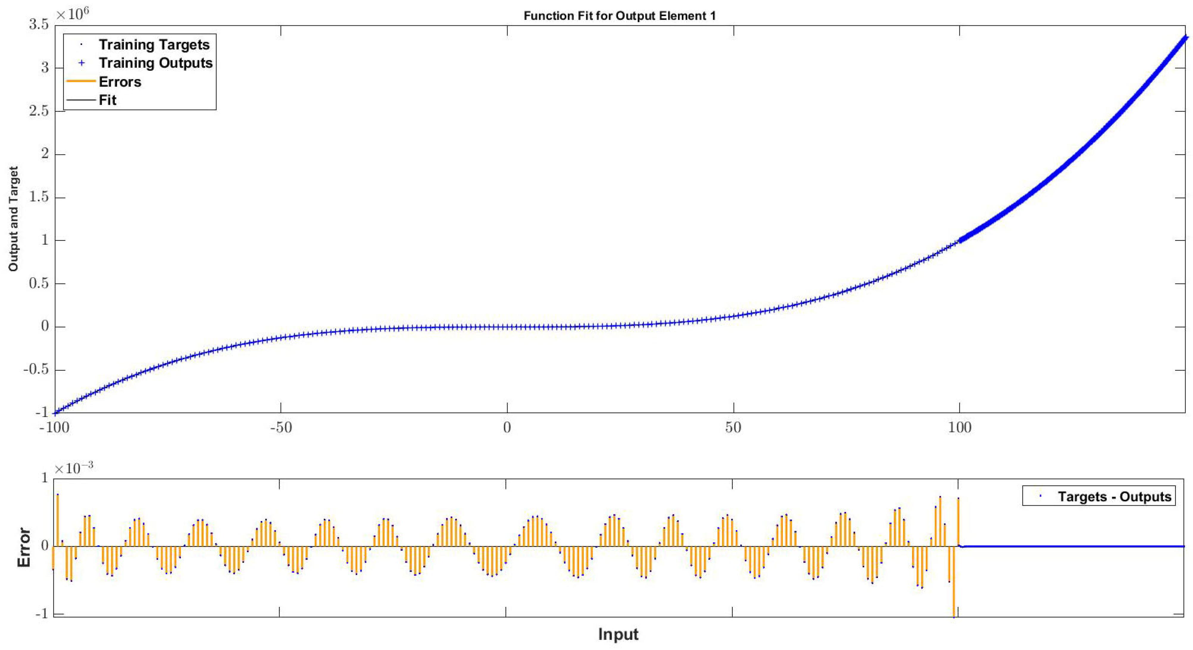
Figure 1 shows that when the network is well trained, it completely covers the graph within the sample range, i.e., it fully predicts the values of the target function. However, as the distance from the boundaries of the training sample increases, the errors become larger, and, accordingly, the graph of the ANN-predicted values moves further and further away from the graph of the target function. Predictions made for values far from the training sample boundaries always have a larger error. Table 1 presents the absolute errors of the neural networks approximating some of the functions considered in the experiments, both near and far from the boundaries of the interval used in the training samples.
In each example, it turned out that near the boundaries of the samples, the errors of the neural networks were minimal, and the further we moved away from these boundaries, the larger the errors became.
For the function
y = x 1 x + 1
the smallest error values were for N e t ( 101 ) and N e t ( 100.01 ), but this was due to the fact that x = 100.01 and x = 101 were included in the interval from which the training samples were taken. From the values of x outside the training sample interval, the minimum error was again achieved near the boundaries.
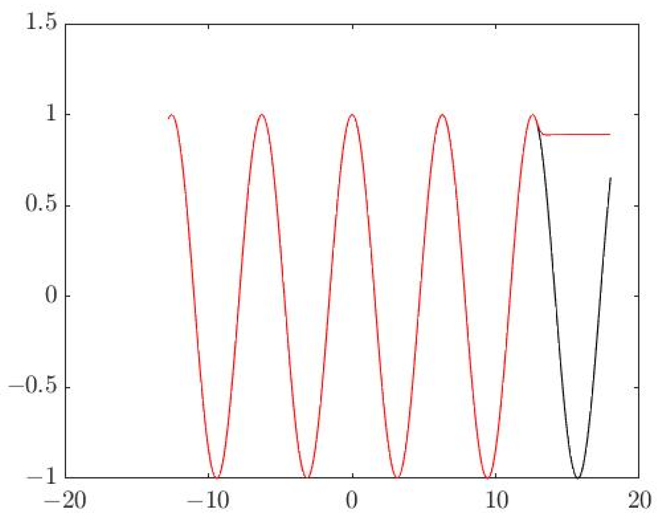
It is noteworthy that for the periodic functions, when the distance from the boundary of the training segment increases, a fluctuation of the prediction error is observed. This is due precisely to the periodic nature of these types of functions (Figure 2 and Table 2). The graph of the real target function on Figure 2 is in black color and the predictions of the trained ANN are shown in red color.

4. New Concepts and Definitions Needed to Describe the Iterative Algorithm

A N e t neural network is said to be trained on a sampling of input–output samples if it has been trained with an algorithm that can find weight and threshold values in the network that suitably minimize the error function of the sample interpolation and the test.
In general, for a single training of a neural network, the prediction error is not zero. If the network architecture, the sampling, the transfer functions, or the algorithms selected are not appropriate, the errors can be significant and can render the neural network useless.
Figure 3 shows a neural network with inappropriate architecture (one hidden layer with two neurons) which has undergone a single training using the Levenberg–Marquardt algorithm for the interpolation of the function y = l o g ( x ) . The transfer function is a hyperbolic tangent. The number of training epochs was determined by the algorithm, and default values of 0.01, 0.1 and 0.5 were used for the training rate. Subsequently, after the training, when calculating the target function, it is still possible for the neural network to make errors and deviate from the real functional values of the interpolated dependence. This, in turn, would inevitably affect the predictive capabilities of such an ANN beyond the boundaries of the training sample used.
Definition 1. 
(A neural network perfectly trained on the dataset.) We will call the artificial neural network perfectly trained on the sampling of input–output samples  D = X j ;   t j = F X j j = 1 m  only after the training has been conducted.
N e t X j = t j ,     X j ;   t j D ,   j = 1 ,   2 , m .
According to Definition 1, the N e t network is perfectly trained on a given sampling if, when calculating the values of the functional dependence F at each of the sampling nodes, the error is zero.
On the other hand, we must keep in mind that for each sampling of input–output samples, an infinite number of neural networks can be found and subsequently trained. Some of the neural networks will interpolate the sample with large errors, others will perform better, and some of them will be perfectly trained. These neural networks may have different architectures and different numbers of weights and thresholds. If we consider feedforward neural networks, which receive n   input signals, have   r hidden layers, and in each of which there is an equal number of neurons ( q ), we will see that the number of all the connections in the network, i.e., the weights and thresholds that are subject to adjustments by the training algorithms, is as follows:
p = r 1 q 2 + r + n + k q + k ,
where k is the number of output neurons. In another type of architecture, the number of weights and thresholds can be set by a different mathematical expression, but in all cases, it will be the number N .
Definition 2. 
(Capacity of the architecture of an artificial neural network.) The number of all the weights and thresholds in the artificial network  N e t  will be called the capacity of the  N e t  architecture, or simply the capacity of the Net, and will be denoted by   p N e t .
It is obvious that the minimum capacity of the architecture of a network is p = 1 , and this is characteristic of a network consisting of a single neuron with no threshold to which only one input stimulus is supplied. This means that a set consisting of the values of all possible p N e t , though infinite, would be bounded from below, with an exact lower bound of 1. It should be noted that the capacity of the architecture should not only be related to the number of hidden layers and neurons they contain, but also to the connections in the network itself. For example, the capacity of a neural network with more layers may be lower than the capacity of a neural network with fewer layers, but which also has feedback.
The introduction of the “capacity of architecture” concept enables each particular neural network N e t to be associated with a number p N e t , which allows us to explore neural networks through ordered pairs ( N e t ,   p N e t ) . Let be the set of ordered pairs of all the kinds of networks and their respective capacities that can be trained on the specific sampling
= N e t i , p N e t i / i ,   p N e t i N .
The set of all the kinds of values of these networks is p = { p N e t i } i N . The minimum value of the capacity of an architecture is 1; therefore p is bounded from below, i.e.,
min p N e t i i N 1 .
Let = N e t i , p N e t i /   i ,   p N e t i N be a set containing the ordered pairs of all the neural networks trained on the sample D = X j ;   t j = F X j j = 1 m and their respective capacities.
Definition 3. 
(Optimal artificial neural network on dataset.) The artificial neural network   N e t  is optimal for the sampling  D  only after the training has been conducted as follows:
(1)
N e t  is perfectly trained on  D  , i.e., condition (4) is satisfied, and
(2)
p Net = min { p N e t i } i N ,
where the ordered pair is  N e t , p N e t .
Several optimal neural networks may exist for a single sampling and meet the required conditions of Definition 3, namely, they may be perfectly trained and have minimal capacity. At the same time, optimal neural networks can be of different types, with different functionalities, different numbers of hidden layers, and different numbers of neurons.
According to Definition 3, any network that is optimal for a certain sampling is perfectly trained on the sampling, but not every perfectly trained network is optimal. In other words, the class of optimal networks is much narrower than that of perfectly trained ones.

5. A Method for Extrapolating Continuous Functions with Artificial Neural Networks by Generating New Training Samples

Let us look again at the N e t network trained with m   number of input–output samples of the type
D = X j ; t j = F X j j = 1 m ,
where F X j is a continuous function. Additionally, let the transfer function in the neuron bodies of the N e t also be continuous.
If we assume that the network is perfectly trained on the sample in the interpolation of the target function F X j , statistically represented by D , then according to condition (4),
N e t X j = t j for     X j ; t j D ,   j = 1,2 , m ,
where
X j = ( x j 1 , x j 2 , x j n ) ,   x j k [ α k ,   β k ] ,     α k ,   β k R ,     j = 1,2 , m ,     k = 1,2 , n .
When trying to extrapolate the behavior of F beyond the boundaries of [ α k ,   β k ] , the absolute error of N e t at values of the arguments X m + 1 according to (2) is
ε = N e t X m + 1 F X m + 1 .
For definiteness, let us consider the case   x ( m + 1 ) , k > β k . For values lower than the left boundary α k of the intervals [ α k ,   β k ] , or in cases where some of the new arguments are on the right and others are on the left, the reasoning is analogical. The larger the difference
β k = x m + 1 , k β k
the larger we can expect the error ε to be. On the other hand, for the perfectly trained N e t and for Β = β 1 ,   β 2 , β n , we have
N e t Β = F Β N e t β 1 ,   β 2 , β n = F β 1 ,   β 2 , β n .
Due to the continuous nature of the transfer function used in N e t , the N e t X j , as a composition of continuous functions, is also a continuous function. Therefore,
lim β p 0 N e t β 1 + β 1 , β 2 + β 2 , β n + β n = N e t β 1 ,   β 2 , β n
On the other hand, due to the continuous nature of the target function F , we have
lim β p 0 F β 1 + β 1 , β 2 + β 2 , β n + β n = F β 1 ,   β 2 , β n .
Then, from (10), (11), and (12), it follows that
lim β p 0 N e t β 1 + β 1 , β 2 + β 2 , β n + β n = lim β p 0 F β 1 + β 1 , β 2 + β 2 , β n + β n
In other words, although N e t x j 1 , x j 2 , x j n and F x j 1 , x j 2 , x j n are different functions, in an infinitesimal neighborhood of the point ( β 1 ,   β 2 , β n ) , they tend to the same number. In this neighborhood, according to (9) and (13), we can assume that
F X m + 1 = N e t X m + 1   F x m + 1 , 1 , x m + 1 , 2 , x m + 1 ,   n = N e t x ( m + 1 ) , 1 , x ( m + 1 ) , 2 , x ( m + 1 ) ,   n ,
which gives us sufficient reason to form a new model for N e t , created by N e t itself:
D 1 = X m + 1 ;   t m + 1 = N e t X m + 1 .
If the network is perfectly trained on the new sample D D 1 and we repeat the process, deviating an infinitesimal distance from the boundaries of the new intervals [ α k ,   β k + β k ] , in which the independent variables x j 1 , x j 2 , x j n   ( j = 1 ,   2 , ,   m + 1 ) fall, we will discover an additional new pattern for the training of N e t :
D 2 = X m + 2 ;   t m + 2 = N e t X m + 2 ,
in which the point X m + 2 is infinitely close to the point X m + 1 .
Continuing in this way, we can create an infinite number of new training samples that form the new sampling
D D 1   D 2 D 3 ,
with which the neural network can be trained.
It is obvious that due to the infinite number of iterations, no algorithm can be created that will gradually approach the remote value X t a r g e t and forecast F X t a r g e t because this would take infinite time and resources. However, we could implement an algorithm where the value to be predicted is approached with steps that are as small as possible ( β k ). Bearing in mind that in this case β k are not infinitely small numbers, Equation (13) will not be exactly satisfied, and an additional error term— e —will appear:
N e t β 1 + β 1 , β 2 + β 2 , β n + β n = F β 1 + β 1 , β 2 + β 2 , β n + β n + e ,   for which l i m β k 0 e = 0
In other words, the smaller the steps with which we approach the prediction values, the smaller this error will be.
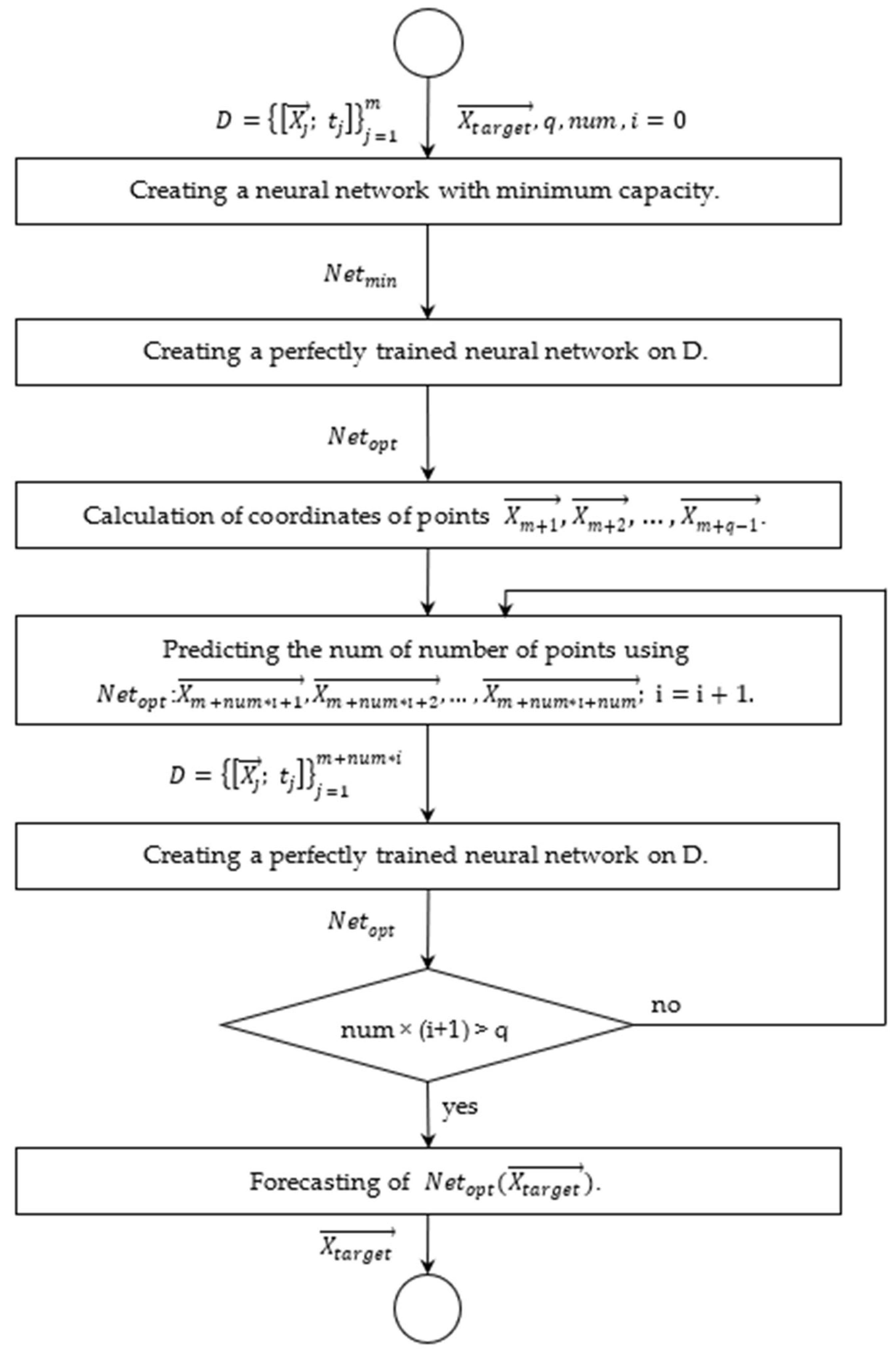
The algorithm used for iterative forecasting aims to predict the values of the target function using a neural network for point X t a r g e t = x t a r g e t , 1 , x t a r g e t , 2 , x t a r g e t ,   n which is relatively far from the sampling boundaries. It consists of four main stages (Figure 4).
(1)
Creating an efficient artificial neural network with minimum capacity on the initial sample
In this stage, suitable single-layer and multi-layer networks are sought. The initial sample is now divided into three groups: 70% of the sample volume is used for training, 15% is used for the validation of the learning process, and 15% is used to independently test the networks that are found. The search of the neural network is carried out by gradually increasing the complexity of the architecture, i.e., the number of layers and the number of neurons are increased gradually with or without another heuristic algorithm until their upper limits are reached [53]. From the neural networks created in this way, the most efficient one (with a predetermined minimum error) is selected. Successive increases in the number of layers and the number of neurons allows the creation of an initial network that is adequately efficient and has minimal capacity.
(2)
Creating a perfectly trained artificial neural network
In this stage, the suitable neural network that was found is repeatedly trained using 100% of the sampling set. The goal of training the neural network using all of the samples is to achieve as good an interpolation as possible within the given sampling. Repeated training of the neural network is performed, which is equivalent to increasing the number of epochs, but which allows the process to be stopped upon reaching an error plateau. The goal at this stage is to create a perfectly trained network, i.e., and optimal network with minimum capacity.
At the end of the second stage, the trained ANN has an optimal topology and perfectly interpolates within the sampling boundaries.
(3)
Generating new samples outside the initial sampling
  • The number q   ( q N )   of prediction points that lie between the sample boundaries and the target prediction point X t a r g e t = x ( m + q ) , 1 , x ( m + q ) , 2 , x ( m + q ) ,   n is determined. The available computing resources and time, as well as the user settings, are important for determining the number of points q . A greater number of points leads to more accurate prediction results.
  • The intermediate points X m + 1 ,   X m + 2 ,   , X m + q 1 which are evenly spaced between X m and X t a r g e t are calculated. With different modifications to the algorithm, these points may be calculated differently and therefore they may not be evenly distributed.
  • The following activities are performed iteratively until the target point is reached:
    Using the current AN, one or more points are predicted, successively taking the points closest to the boundary. The number of these points is set by the user.
    The newly obtained input–output samples are added to the neural network training dataset.
    A neural network is perfectly trained on the updated dataset.
(4)
Prediction
With an AN trained on D = X j ;   t j = F X j j = 1 m + q 1 , X t a r g e t is predicted.
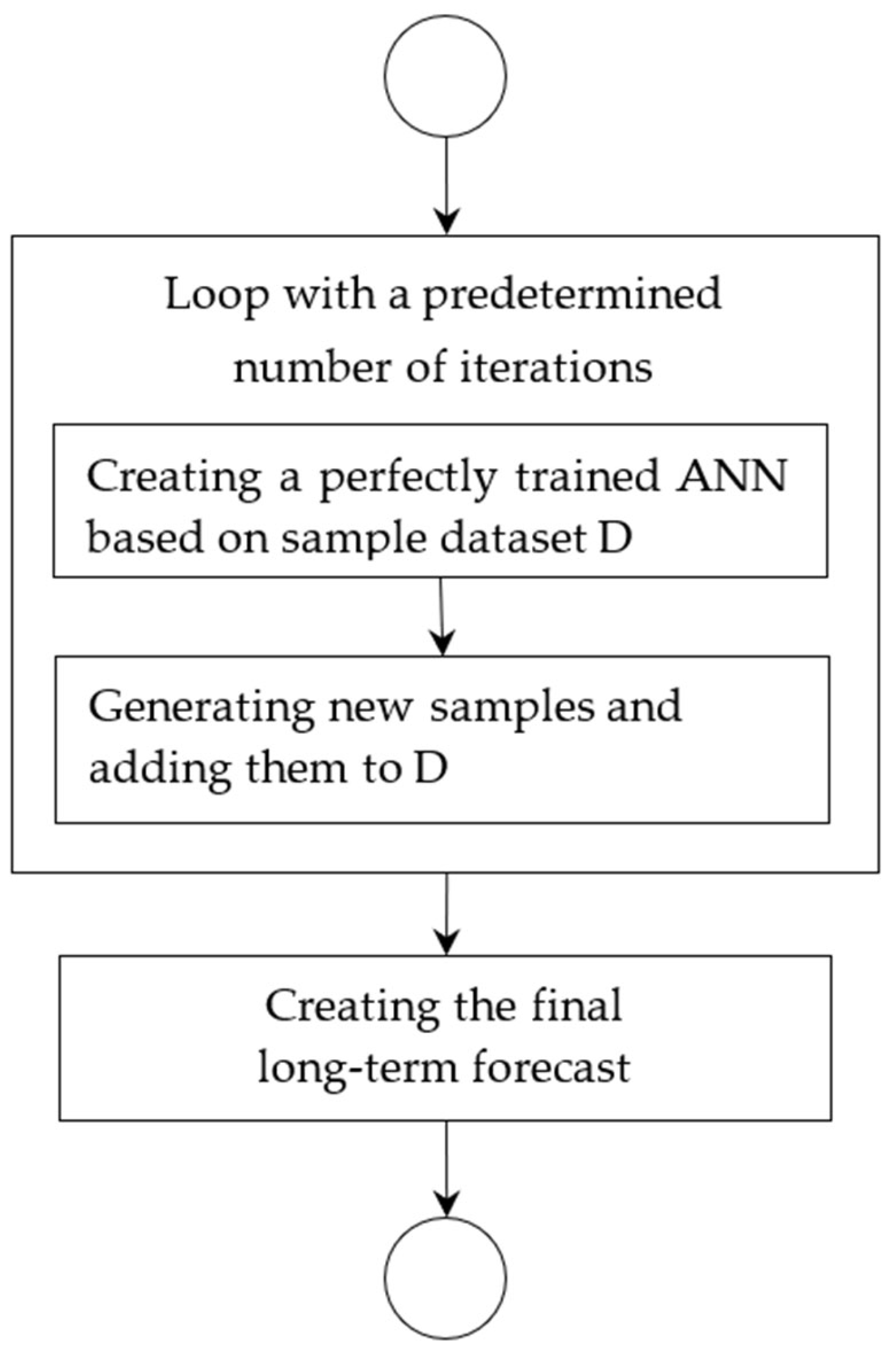
A simplified representation of the algorithm steps is shown in Figure 5.

6. Experiments and Discussion

The described algorithm was implemented using MATLAB scripts, and after their execution a comparative analysis of the results was carried out. Error reduction was observed in all the approximations studied, even when they concerned functions that are difficult to work with in this regard, such as periodic functions. For more convenient visualization and tracking of the changes, the following color code is used in the graphs of the functions approximated by the neural networks:
Axioms 12 00759 i001Represents the graph of the real target function F. The algorithms have not yet been started and the network Net has not been created.
Axioms 12 00759 i002The algorithm has completed stage (1) and a minimum capacity approximating the neural network Net trained on the original sample is created.
Axioms 12 00759 i003Represents the graph of the approximating neural network Net after the algorithm has completed step (2) and the network has been optimized, i.e., after it has been perfectly trained on the sample and the minimum capacity has been obtained.
Axioms 12 00759 i004Represents the graph of the approximating neural network Net after the algorithm has completed stage (3). The network is perfectly trained on the samples outside the initial dataset.
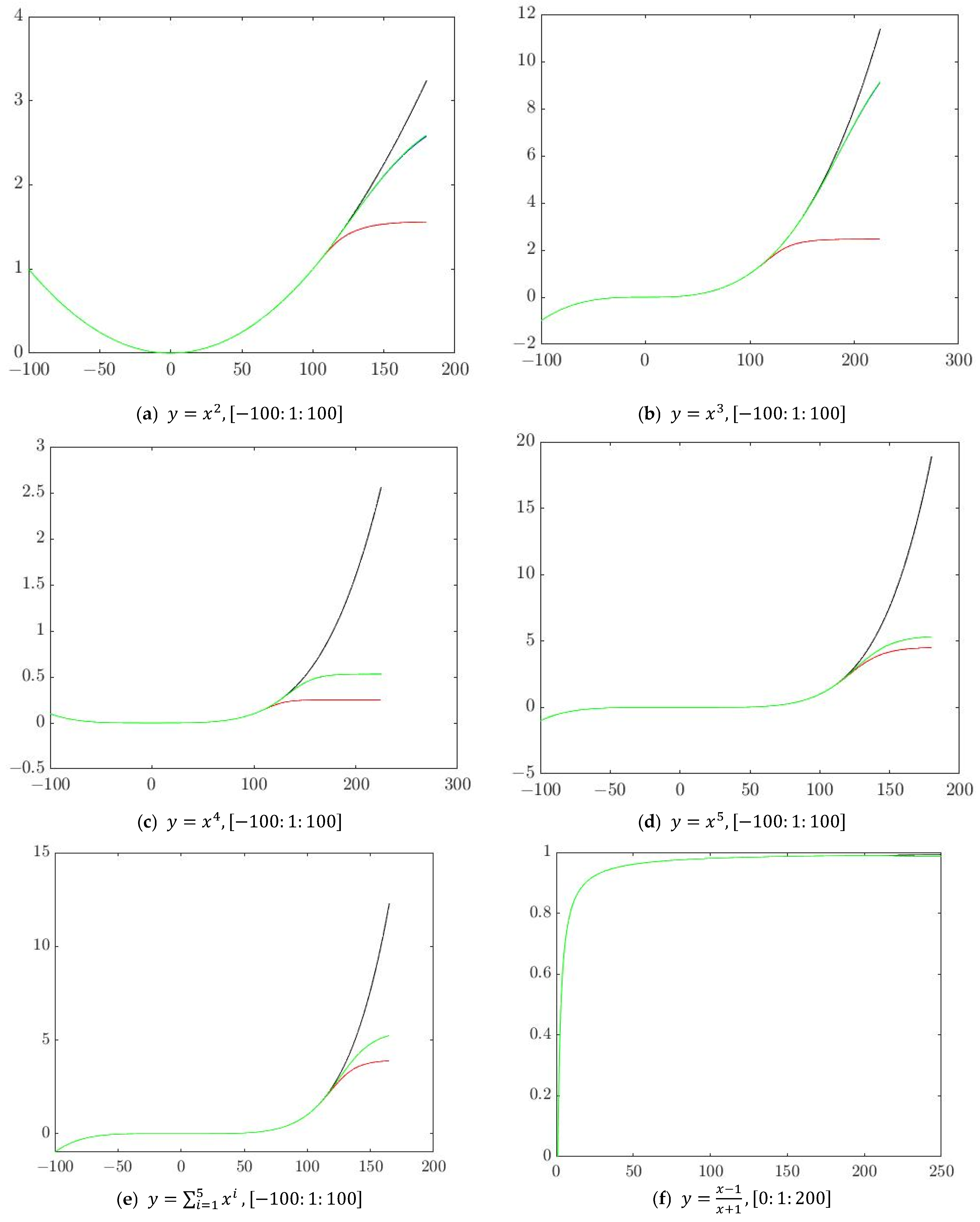
Using the indicated color code, the results of the approximations of the neural network found initially and the same neural network after it has passed through the stages of the proposed algorithm can be viewed and compared in the graphs of Figure 6. The neural networks are trained using the Levenberg–Marquardt algorithm, and the transfer function of the hidden layer neurons is the tangent hyperbolic function. The algorithm itself determined the number of iterations (epochs) needed and selected them by automatically changing the speed at which error gradient descent was performed.
The presented results illustrate some of the experiments conducted using single-variable functions. Similar results were obtained in the experiments conducted using multivariable functions. In all cases, the network trained with the algorithm produced better predictive results than the ANN that was initially found. For some of the functions, including the three examples
y = 2 x + 1 ,   y = x 1 x + 1 ,   and   y = x 3 ,
the interpolations and predictions of the ANN almost completely matched the corresponding target function both within and outside the training interval. To further verify the qualities of the predictive algorithm, we investigate the network performance indicator
e f f i c i e n c y = 1 p e r f o r m a n c e ,
where p e r f o r m a n c e is the aggregate performance expressed as errors of the ANN during training, validation, and testing. Furthermore, a comparison was made between the mean absolute percentage errors (MAPEs) of the network in predicting the value of the target function at a specific point x = 150 (which is outside the sample range) both before and after it had passed through the stages of the algorithm. The results are presented in Table 3.
Figure 7 presents the neural networks’ approximations for the y = x 3 function. The bold right part of the graphs shows the additional training samples that were built.
The proposed algorithm can also be used for periodic functions such as y = sin x and y = cos x , which are traditionally difficult to approximate using feedforward neural networks. Even in these cases, the use of the iteration algorithm improves the quality of the networks used (Table 4).
Experiments on the performance of the algorithm were also conducted using multivariable functions of different types. The two-variable linear function
y = 2 x 1 + 3 x 2 + 1
was studied.
For its interpolation, the neural network N e t   was trained in the intervals
x 1 100 : 1 : 100 ,   x 2 [ 1 : 1 : 201 ] .
Initially, the efficiency of the ANN was 3.67 × 10¹¹, and the absolute percentage error (APE) of the prediction for value y at point   x 1 = 150 ,   x 2 = 250 was 2.17%. After N e t passed through the stages of the algorithm, the efficiency of the network became 7.07 × 10¹¹, and the APE of the prediction for value y at point   x 1 = 150 ,   x 2 = 250 became 1.65%.
For the function
y = x 1 + x 2 + x 3 + x 1 x 2 x 3
a neural network was trained in the intervals
x 1 100 : 1 : 100 ,   x 2 1 : 1 : 201 ,   x 3 [ 0.03 : 0.03 : 6.03 ] .
At the beginning, the efficiency was 1.25 × 10⁸ and the absolute percent error for predicting at point   x 1 = 150 ,   x 2 = 250 ,   x 3 = 10   was 30.57%. After the additional training of the ANN using the training samples created by the network itself, the prediction values approached the target values: the efficiency became 3.97 × 10¹⁰ and the error decreased to 15.68%.
In many cases, the absolute percent errors showed multifold decreases. For example, when approximating the functions
y = x 2   and   y = x 1 x + 1
the errors of the initial networks were 31.81% and 0.51%, respectively. After applying the algorithm, the respective errors were reduced to values of 6.34% and 0.14%. In some cases, the improvements to the original network were so good that even far outside the range of the given sampling, the approximating neural network almost completely covered the real function in the area between the sample boundary and the point up to which it constructed new samples itself (Figure 8).
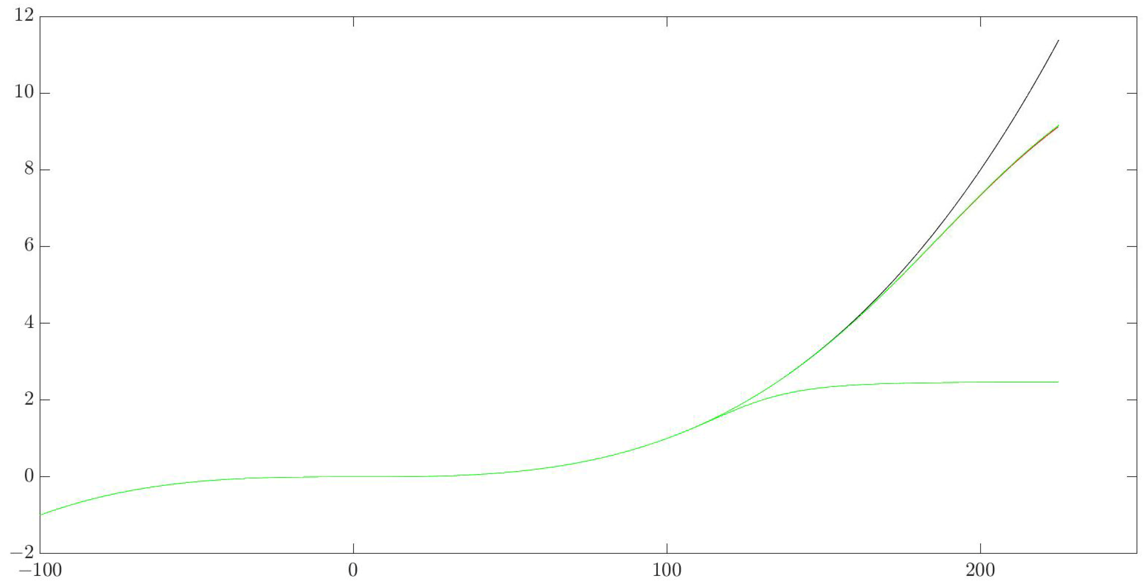
Figure 8 presents an approximation of the function y = x 3 . The training of the neural network is carried out in the interval x 1 100 : 1 : 100 , and the goal of the network is to predict the value y 150 . Almost immediately after the end of the sampling, the initial network (in red) starts to deviate from the graph of the target function, and its prediction for y 150 has a large error. In the second stage, the algorithm optimizes the network. The approximation of the target function through the optimal network is shown in blue. During the third stage, the optimal network starts building the additional samples up to point x = 150 and is continuously trained, both on the main sampling and on the newly created samples. The approximation of the target function at this stage of the algorithm is shown in green. Although very close to the optimal network (in blue), the final version (in green) has improved qualities, and a comparison with the initial network (in red) shows an error reduction from 31.12% to 0.25%.
When working with periodic functions which are typically difficult to approximate, the algorithm showed something interesting (Figure 9). With feedforward neural networks. it is quite challenging to transform the initial network into an optimal one, i.e., one that is perfectly trained on the sample and has minimum capacity. The graphs of the approximation of the initial network (in red) and the optimal network (in blue) almost match, and immediately after the end of the sampling, they start to predict with a large error. However, as the optimal neural network starts to approach the desired external point with additional samples that it creates itself, and as it is retrained on all the data, its performance starts to improve (in green).

7. Conclusions

In general, methods for the approximation and prediction of processes involve difficulties and produce more inaccurate approximation results when predicting values far from the boundaries of statistical samples. This applies to both mathematical methods and neural networks (which are representative of artificial intelligence methods). The iterative prediction algorithm proposed in this paper is based on two assumptions. One is that predictions near the statistical sampling have much smaller errors than those far from the sampling. The second assumption is that a neural network can generate additional training samples and use them to retrain itself in order to get closer to an initially distant prediction point. Numerous practical experiments were conducted on single-variable and multi-variable functions of different types, and a comparison was made between the predictive abilities of the neural networks before and after the application of the iterative algorithm. The results showed an increase in efficiency and a reduction in the errors of the neural networks that passed through the stages of the algorithm.

Author Contributions

Conceptualization, K.Y., E.H. and S.H.; methodology, K.Y., E.H. and S.H.; validation, S.H. and S.C.; formal analysis, K.Y., E.H. and S.C.; investigation, K.Y., E.H., S.H. and S.C.; data curation, K.Y. and S.C; writing—original draft preparation, K.Y. and E.H.; writing—review and editing, S.H. and S.C.; supervision, E.H. and S.H.; project administration, E.H.; funding acquisition, E.H. All authors have read and agreed to the published version of the manuscript.

Funding

This work was partly funded by the MUPD23-FMI-021 and SP23-FMI-008 projects of the Research Fund of the University of Plovdiv “Paisii Hilendarski”.

Data Availability Statement

Not applicable.

Conflicts of Interest

The authors declare no conflict of interest.

References

  1. Celik, S.; Inci, H.; Sengul, T.; Sogut, B.; Sengul, A.; Taysi, M. Interpolation method for live weight estimation based on age in Japanese quails. Rev. Bras. Zootec. 2016, 45, 445–450. [Google Scholar] [CrossRef] [Green Version]
  2. Burden, R.L.; Faires, J.D. Interpolation & Polynomial Approximation/Lagrange Interpolating Polynomials II. In Numerical Analysis, 9th ed.; Faires, R.L., Ed.; Brooks/Cole, Cengage Learning: Dublin, Ireland, 2011. [Google Scholar]
  3. Mutombo, N.M.-A.; Numbi, B.P. Development of a Linear Regression Model Based on the Most Influential Predictors for a Research Office Cooling Load. Energies 2022, 15, 5097. [Google Scholar] [CrossRef]
  4. Guerard, J. Regression Analysis and Forecasting Models. In Introduction to Financial Forecasting in Investment Analysis; Springer: Berlin/Heidelberg, Germany, 2013. [Google Scholar] [CrossRef]
  5. Schleifer, A. Forecasting with Regression Analysis; Product #: 894007-PDF-ENG; Harvard Business Publishing: Harvard, MA, USA, 1993. [Google Scholar]
  6. Peña, D.; Tiao, G.; Tsay, R.A. Course in Time Series Analysis; Wiley: Hoboken, NJ, USA, 2000; ISBN 978-0-471-36164-0. [Google Scholar]
  7. Yaffee, R.; McGee, M. Introduction to Time Series Analysis and Forecasting with Applications of SAS and SPSS; Academic Press: Cambridge, MA, USA, 2000; ISBN 0127678700. [Google Scholar]
  8. Brockwell, P.; Davis, R. Introduction to Time Series and Forecasting; Springer: Berlin/Heidelberg, Germany, 2002; ISBN 0-387-95351-5. [Google Scholar]
  9. Zhou, H.; Wang, T.; Zhao, H.; Wang, Z. Updated Prediction of Air Quality Based on Kalman-Attention-LSTM Network. Sustainability 2023, 15, 356. [Google Scholar] [CrossRef]
  10. Ly, R.; Traore, F.; Dia, K. Forecasting commodity prices using long-short-term memory neural networks. IFPRI Discuss. Pap. 2021, 2000, 26. [Google Scholar] [CrossRef]
  11. Zhang, K.; Hong, M. Forecasting crude oil price using LSTM neural networks. Data Sci. Financ. Econ. 2022, 2, 163–180. [Google Scholar] [CrossRef]
  12. Wei, J.; Zou, K. EDA: Easy Data Augmentation Techniques for Boosting Performance on Text Classification. In Proceedings of the ICLR 2019-7th International Conference on Learning Representations, Hong Kong, China, 3–7 November 2019; pp. 6382–6388. [Google Scholar] [CrossRef] [Green Version]
  13. Şahin, G.G.; Steedman, M. Data Augmentation via Dependency Tree Morphing for Low-Resource Languages. In Proceedings of the 2018 Conference on Empirical Methods in Natural Language Processing, Brussels, Belgium, 31 October–4 November 2018; pp. 5004–5009. [Google Scholar] [CrossRef]
  14. Fadaee, M.; Bisazza, A.; Monz, C. Data Augmentation for Low-Resource Neural Machine Translation. In Proceedings of the 55th Annual Meeting of the Association for Computational Linguistics, Vancouver, BC, Canada, 30 July–4 August 2017; pp. 567–573. [Google Scholar] [CrossRef] [Green Version]
  15. Sugiyama, A.; Yoshinaga, N. Data augmentation using back-translation for context-aware neural machine translation. In Proceedings of the Fourth Workshop on Discourse in Machine Translation (DiscoMT 2019), Hong Kong, China, 6–9 November 2019; pp. 35–44. [Google Scholar] [CrossRef]
  16. Shorten, C.; Khoshgoftaar, T.M.; Furht, B. Text data augmentation for deep learning. J. Big Data 2021, 8, 101. [Google Scholar] [CrossRef] [PubMed]
  17. Abdali, S.; Mukherjee, S.; Papalexakis, E. Vec2Node: Self-Training with Tensor Augmentation for Text Classification with Few Labels. Mach. Learn. Knowl. Discov. Databases 2023, 13714, 571–587. [Google Scholar] [CrossRef]
  18. Kwon, S.; Lee, Y. Explainability-Based Mix-Up Approach for Text Data Augmentation. ACM Trans. Knowl. Discov. Data 2023, 17, 13. [Google Scholar] [CrossRef]
  19. Saha, P.; Logofatu, D. Efficient Approaches for Data Augmentation by Using Generative Adversarial Networks. Eng. Appl. Neural Netw. 2022, 1600, 386–399. [Google Scholar] [CrossRef]
  20. Summers, C.; Dinneen, M.J. Improved mixed-example data augmentation. In Proceedings of the 2019 IEEE Winter Conference on Applications of Computer Vision (WACV), Waikoloa, HI, USA, 7–11 January 2019; pp. 1262–1270. [Google Scholar] [CrossRef] [Green Version]
  21. Kaur, P.; Khehra, B.S.; Mavi, E.B.S. Data augmentation for object detection: A review. In Proceedings of the 2021 IEEE International Midwest Symposium on Circuits and Systems (MWSCAS), Lansing, MI, USA, 9–11 August 2021; pp. 537–543. [Google Scholar] [CrossRef]
  22. Zoph, B.; Cubuk, E.D.; Ghiasi, G.; Lin, T.Y.; Shlens, J.; Le, Q.V. Learning Data Augmentation Strategies for Object Detection. In Proceedings of the 16th European Conference, Glasgow, UK, 23–28 August 2020; Lecture Notes in Computer Science; Vedaldi, A., Bischof, H., Brox, T., Frahm, J.M., Eds.; Springer: Cham, Switzerland, 2020; Volume 12372, pp. 566–583. [Google Scholar] [CrossRef]
  23. Fawzi, A.; Samulowitz, H.; Turaga, D.; Frossard, P. Adaptive data augmentation for image classification. In Proceedings of the 2016 IEEE International Conference on Image Processing (ICIP), Phoenix, AZ, USA, 25–28 September 2016; pp. 3688–3692. [Google Scholar] [CrossRef] [Green Version]
  24. Chlap, P.; Min, H.; Vandenberg, N.; Dowling, J.; Holloway, L.; Haworth, A. A review of medical image data augmentation techniques for deep learning applications. J. Med. Imaging Radiat. Oncol. 2021, 65, 545–563. [Google Scholar] [CrossRef]
  25. Nalepa, J.; Marcinkiewicz, M.; Kawulok, M. Data augmentation for brain-tumor segmentation: A review. Front. Comput. Neurosci. 2019, 13, 83. [Google Scholar] [CrossRef] [Green Version]
  26. Chen, Y.; Yang, X.-H.; Wei, Z.; Heidari, A.A.; Zheng, N.; Li, Z.; Chen, H.; Hu, H.; Zhou, Q.; Guan, Q. Generative adversarial networks in medical image augmentation: A review. Comput. Biol. Med. 2022, 144, 105382. [Google Scholar] [CrossRef]
  27. Zhao, J.; Cheng, Y.; Cheng, Y.; Yang, Y.; Zhao, F.; Li, J.; Liu, H.; Yan, S.; Feng, J. Look across elapse: Disentangled representation learning and photorealistic cross-age face synthesis for age-invariant face recognition. Proc. AAAI Conf. Artif. Intell. 2019, 33, 9251–9258. [Google Scholar] [CrossRef] [Green Version]
  28. Zhao, J.; Cheng, Y.; Xu, Y.; Xiong, L.; Li, J.; Zhao, F.; Jayashree, K.; Pranata, S.; Shen, S.; Xing, J.; et al. Towards pose invariant face recognition in the wild. In Proceedings of the IEEE Conference on Computer Vision and Pattern Recognition, Salt Lake City, UT, USA, 18–23 June 2018; pp. 2207–2216. [Google Scholar] [CrossRef]
  29. Tran, L.; Yin, X.; Liu, X. Disentangled representation learning gan for pose-invariant face recognition. In Proceedings of the IEEE Conference on Computer Vision and Pattern Recognition, Honolulu, HI, USA, 21–26 July 2017; pp. 1415–1424. [Google Scholar] [CrossRef]
  30. Chen, X.; Wang, G.; Guo, H.; Zhang, C. Pose guided structured region ensemble network for cascaded hand pose estimation. Neurocomputing 2020, 395, 138–149. [Google Scholar] [CrossRef] [Green Version]
  31. Baek, S.; Kim, K.I.; Kim, T.K. Augmented skeleton space transfer for depth-based hand pose estimation. In Proceedings of the IEEE Conference on Computer Vision and Pattern Recognition, Salt Lake City, UT, USA, 18–23 June 2018; pp. 8330–8339. [Google Scholar] [CrossRef] [Green Version]
  32. Chen, L.; Lin, S.Y.; Xie, Y.; Lin, Y.Y.; Fan, W.; Xie, X. DGGAN: Depth-image guided generative adversarial networks for disentangling RGB and depth images in 3D hand pose estimation. In Proceedings of the IEEE/CVF Winter Conference on Applications of Computer Vision, Village, CO, USA, 1–5 March 2020; pp. 411–419. [Google Scholar] [CrossRef]
  33. He, W.; Xie, Z.; Li, Y.; Wang, X.; Cai, W. Synthesizing depth hand images with GANs and style transfer for hand pose estimation. Sensors 2019, 19, 2919. [Google Scholar] [CrossRef] [PubMed] [Green Version]
  34. Cader, A. The Potential for the Use of Deep Neural Networks in e-Learning Student Evaluation with New Data Augmentation Method. Artif. Intell. Educ. 2020, 12164, 37–42. [Google Scholar] [CrossRef]
  35. Cochran, K.; Cohn, C.; Hutchins, N.; Biswas, G.; Hastings, P. Improving Automated Evaluation of Formative Assessments with Text Data Augmentation. Artif. Intell. Educ. 2022, 13355, 390–401. [Google Scholar] [CrossRef]
  36. Maharana, K.; Mondal, S.; Nemade, B. A review: Data pre-processing and data augmentation techniques. Glob. Transit. Proc. 2022, 3, 91–99. [Google Scholar] [CrossRef]
  37. Ostertagova, E. Modelling Using Polynomial Regression. Procedia Eng. 2012, 48, 500–506. [Google Scholar] [CrossRef] [Green Version]
  38. Hyndman, R.; Athanasopoulos, G. Forecasting: Principles and Practice; OTexts: Melbourne, VI, Australia, 2013; ISBN 0987507109. [Google Scholar]
  39. Chollet, F. Deep Learning with Python; Manning: Shelter Island, NY, USA, 2021; ISBN 1617296864. [Google Scholar]
  40. Bandara, K.; Bergmeir, C.; Smyl, S. Forecasting across time series databases using recurrent neural networks on groups of similar series: A clustering approach. Expert Syst. Appl. 2020, 140, 112896. [Google Scholar] [CrossRef] [Green Version]
  41. Taylor, S.; Letham, B. Forecasting at Scale. Am. Stat. 2018, 72, 37–45. [Google Scholar] [CrossRef]
  42. Bandara, K.; Hewamalage, H.; Liu, Y.-H.; Kang, Y.; Bergmeir, C. Improving the accuracy of global forecasting models using time series, data augmentation. Pattern Recognit. 2021, 120, 108148. [Google Scholar] [CrossRef]
  43. Goodfellow, I.; Pouget-Abadie, J.; Mirza, M.; Xu, B.; Warde-Farley, D.; Ozair, S.; Courville, A.; Bengio, Y. Generative adversarial networks. Commun. ACM 2020, 63, 139–144. [Google Scholar] [CrossRef]
  44. Mumuni, A.; Mumuni, F. Data augmentation: A comprehensive survey of modern approaches. Array 2022, 16, 100258. [Google Scholar] [CrossRef]
  45. Yoon, J.; Jordon, J.; Schaar, M. GAIN: Missing Data Imputation using Generative Adversarial Nets. arXiv 2018, arXiv:1806.02920. [Google Scholar] [CrossRef]
  46. Aziira, A.; Setiawan, N.; Soesanti, I. Generation of Synthetic Continuous Numerical Data Using Generative Adversarial Networks. J. Phys. Conf. Ser. 2020, 1577, 012027. [Google Scholar] [CrossRef]
  47. Yean, S.; Somani, P.; Lee, B.; Oh, H. GAN+: Data Augmentation Method using Generative Adversarial Networks and Dirichlet for Indoor Localisation. In Proceedings of the IPIN 2021 WiP Proceedings, Lloret de Mar, Spain, 12–13 September 2021. [Google Scholar]
  48. Yean, S.; Somani, P.; Lee, B.; Oh, H. Numeric Data Augmentation using Structural Constraint Wasserstein Generative Adversarial Networks. In Proceedings of the 2020 IEEE International Symposium on Circuits and Systems (ISCAS), Seville, Spain, 12–14 October 2020; pp. 1–6. [Google Scholar] [CrossRef]
  49. Moreno-Barea, F.; Jerez, J.; Franco, L. Improving classification accuracy using data augmentation on small data sets. Expert Syst. Appl. 2020, 161, 113696. [Google Scholar] [CrossRef]
  50. Moreno-Barea, F.J.; Jerez, J.M.; Franco, L. A Parallel Hybrid Neural Network with Integration of Spatial and Temporal Features for Remaining Useful Life Prediction in Prognostics. IEEE Trans. Instrum. Meas. 2023, 72, 3501112. [Google Scholar] [CrossRef]
  51. Zhang, J.; Li, X.; Tian, J.; Luo, H.; Yin, S. An integrated multi-head dual sparse self-attention network for remaining useful life prediction. Reliab. Eng. Syst. Saf. 2023, 233, 109096. [Google Scholar] [CrossRef]
  52. Zhang, J.; Jiang, Y.; Li, X.; Luo, H.; Yin, S.; Kaynak, O. Remaining Useful Life Prediction of Lithium-Ion Battery with Adaptive Noise Estimation and Capacity Regeneration Detection. IEEE/ASME Trans. Mechatron. 2023, 28, 632–643. [Google Scholar] [CrossRef]
  53. Yotov, K.; Hadzhikolev, E.; Hadzhikoleva, S.; Cheresharov, S. Finding the Optimal Topology of an Approximating Neural Network. Mathematics 2023, 11, 217. [Google Scholar] [CrossRef]
Figure 1. Graphs of the approximations of some functions.
Axioms 12 00759 g001
Figure 2. Graph of approximation of the function y = c o s ( x ) .
Axioms 12 00759 g002
Figure 3. An ineffective network trained to interpolate the function y = l o g x .
Axioms 12 00759 g003
Figure 4. Algorithm for iterative forecasting.
Axioms 12 00759 g004
Figure 5. General diagram of the algorithm stages.
Axioms 12 00759 g005
Figure 6. Results—target functions and initial training intervals of the networks.
Axioms 12 00759 g006aAxioms 12 00759 g006b
Figure 7. Building additional samples for y = x 3 from the end of the training interval at point x = 100 to prediction point x = 150 with step Δ β = 0.1 .
Axioms 12 00759 g007
Figure 8. Approximation of the function y = x 3 .
Axioms 12 00759 g008
Figure 9. Approximation of the function y = cos x   by means of a feedforward neural network.
Axioms 12 00759 g009
Table 1. Changes in the approximations of some types of functions when moving away from the boundaries of the training intervals.
FunctionTraining
Sample
Interval
Absolute
Error at N e t ( 200 )
Absolute
Error at N e t ( 101 )
Absolute
Error at N e t ( 100.01 )
Absolute
Error at N e t ( 101 )
Absolute
Error at N e t ( 300 )
Absolute
Error at N e t ( 500 )
y = 2 x + 1 [−100:1:100]2.4 × 10−11.79 × 10−41.41 × 10−41.81 × 10−43.966.85 × 101
y = x 2 [−100:1:100]1.59 × 1041 × 10−21 × 10−31 × 10−27.35 × 1042.34 × 105
y = x 3 [−100:1:100]5.8 × 1064.844.3 × 10−13.852.35 × 1071.21 × 108
y = x 4 [−100:1:100]1.43 × 1091.22 × 1041.92 × 1022.58 × 1037.86 × 1096.23 × 1010
y = x 5 [−100:1:100]2.9 × 10117.21 × 1053.54 × 1044.12 × 1052.4 × 10123.12 × 1013
y = i = 1 5 x i [−100:1:100]3.06 × 10113.54 × 1092.3 × 1072.77 × 1093.24 × 10113.13 × 1013
y = x 1 x + 1 [0:1:200]3.681.963.29 × 10−63.62 × 10−65.3 × 10−14.08
y = l o g ( x ) [1:0.5:100]--3 × 10−31.1 × 10−21.11.61
y = e x [−100:1:100]1.08 × 10346.62 × 10332.67 × 10157.1 × 10431.94 × 101301.4 × 10217
Table 2. Change in the approximation error of the s i n x and c o s x functions when moving away from the boundaries of the training intervals.
FunctionTraining
Sample
Interval
Absolute
Error at N e t ( 20 )
Absolute
Error at N e t ( 13 )
Absolute
Error at N e t ( 12.85 )
Absolute
Error at N e t ( 15 )
Absolute
Error at N e t ( 18 )
Absolute
Error at N e t ( 20 )
y = s i n ( x ) [−12.8:0.1:12.8]0.77.77 × 10−43.06 × 10−50.782.340.67
y = c o s ( x ) [−12.8:0.1:12.8]0.420.013.49 × 10−41.520.10.35
Table 3. Change in the efficiency and the absolute percentage error of the network in predicting y (150) before and after the network had passed through the algorithm stages.
FunctionTraining
Sample
Interval
Efficiency of the Original
Network N e t
Efficiency of N e t after Passing through the Stages of the Algorithm MAPE of the Initial N e t MAPE of N e t
after Passing through the Stages of the Algorithm
y = 2 x + 1 [−100:1:100]5.88 × 1093.2 × 10120.029%0.00024%
y = x 2 [−100:1:100)7.4 × 1048.8 × 101031.8149%6.3355%
y = x 3 [−100:1:100]7.8 × 10−13 × 10731.1204%0.2488%
y = x 4 [−100:1:100]1.03 × 10−32.73 × 10351.20%13.79%
y = x 5 [−100:1:100]1.8 × 10−81.94 × 10−744.85%37.54%
y = i = 1 5 x i [−100:1:100]2.23 × 10−81.94 × 10−750.61%37.34%
y = x 1 x + 1 [0:1:200]9.25 × 10101.79 × 10150.51%0.14%
y = l o g ( x ) [1:0.5:100]1.32 × 10101.35 × 10137.51%2.56%
Note: The absolute percentage errors of the networks approximating y = x 1 x + 1 are calculated in the prediction of y   ( 250 ) .
Table 4. Changes in the efficiency and the absolute percentage error of the network when predicting the functions y = sin x and y = cos x at point x = 18 .
FunctionTraining
Sample
Interval
Efficiency of the Original
Network N e t
Efficiency of N e t after Passing through the Stages of the Algorithm MAPE of the
Initial N e t
MAPE of N e t
after Passing through the Stages of the Algorithm
y = s i n ( x ) [−12.8:0.1:12.8]5.64 × 10−63.84 × 10−398.11%65.33%
y = c o s ( x ) [−12.8:0.1:12.8]2.51 × 10−52.44 × 10−274.20%32.92%
Disclaimer/Publisher’s Note: The statements, opinions and data contained in all publications are solely those of the individual author(s) and contributor(s) and not of MDPI and/or the editor(s). MDPI and/or the editor(s) disclaim responsibility for any injury to people or property resulting from any ideas, methods, instructions or products referred to in the content.