Abstract
Detecting small targets and handling target occlusion and overlap are critical challenges in weld defect detection. In this paper, we propose the S-YOLO model, a novel weld defect detection method based on the YOLOv8-nano model and several mathematical techniques, specifically tailored to address these issues. Our approach includes several key contributions. Firstly, we introduce omni-dimensional dynamic convolution, which is sensitive to small targets, for improved feature extraction. Secondly, the NAM attention mechanism enhances feature representation in the region of interest. NAM computes the channel-wise and spatial-wise attention weights by matrix multiplications and element-wise operations, and then applies them to the feature maps. Additionally, we replace the SPPF module with a context augmentation module to improve feature map resolution and quality. To minimize information loss, we utilize Carafe upsampling instead of the conventional upsampling operations. Furthermore, we use a loss function that combines IoU, binary cross-entropy, and focal loss to improve bounding box regression and object classification. We use stochastic gradient descent (SGD) with momentum and weight decay to update the parameters of our model. Through rigorous experimental validation, our S-YOLO model demonstrates outstanding accuracy and efficiency in weld defect detection. It effectively tackles the challenges of small target detection, target occlusion, and target overlap. Notably, the proposed model achieves an impressive 8.9% improvement in mean Average Precision (mAP) compared to the native model.
Keywords:
defect detection; S-YOLO model; mathematical techniques; binary cross-entropy; stochastic gradient descent MSC:
68T45
1. Introduction
Welding automation technology and weld defect detection technology are two key technologies in the modernization of the manufacturing industry. They can realize the standardization, automation and intelligence of welding process, improve production efficiency and quality, reduce cost, and adapt to the needs of large-scale production. At present, the commonly used detection methods in weld defect detection tasks are nondestructive testing and image processing. Non-destructive testing methods use physical signals to detect the internal structure of welds, but they have limitations such as expensive equipment, complex operation, and high environmental requirements. Image processing methods use image processing and machine learning techniques to extract features and detect targets from weld surface images, which have lower cost and higher flexibility, but also have limitations such as sensitivity to parameter and feature selection, instability to noise and illumination changes, and poor adaptability to new or complex types of defects. The rapid development of deep learning in recent years brings new opportunities and challenges for weld defect detection. Deep learning techniques can show powerful feature learning and classification capabilities by using a large number of samples [1], and can automatically learn high-level semantic features from images to detect defects.
Deep learning has found important applications and developments in the detection field in the 21st century [2]. Using convolutional neural networks and other structures, it achieves efficient and robust defect detection, which is superior to traditional feature-based methods. AlexNet is an eight-layer convolutional neural network model [3] which won the ImageNet image classification competition in 2012 [4], leading the deep learning revolution in computer vision. R-CNN is a region-based convolutional neural network model [5,6], which first applied deep learning to object detection in 2014 and significantly improved performance on the PASCAL VOC dataset, opening a new era of deep learning-based object detection, but also had drawbacks such as slow speed, complex training, and large memory consumption. Fast R-CNN improved the training process of R-CNN [7], using fully connected layers instead of support vector machine classifiers and bounding box regressors and introducing an RoI pooling layer to achieve end-to-end training. Faster R-CNN is an improved R-CNN model, which uses RPN to generate target candidate regions and shares convolutional layers with feature extraction network, greatly improving the speed and accuracy of object detection, laying the foundation for two-stage algorithms. The YOLO algorithm transforms object detection into a regression problem [8], using a convolutional neural network to directly predict the category and location of objects, eliminating the process of generating candidate regions. The YOLO algorithm has advantages such as fast speed, strong generalization ability, and low background false detection rate, but also has disadvantages such as spatial constraints, difficulty in expansion, and inaccurate localization. YOLOv1 algorithm pioneered single-stage algorithm, providing a new research direction for the object detection field.
In recent years, Mask R-CNN, RetinaNet, CornerNet, and more versions of the YOLO algorithm have promoted the further expansion of deep learning techniques. These methods have proposed some novel and effective ideas and techniques based on the original ones, expanding the scope and difficulty of detection tasks. Mask R-CNN [9] adds a segmentation branch on top of Faster R-CNN to achieve simultaneous object detection and instance segmentation. RetinaNet addresses the problem of positive–negative sample imbalance in single-stage detection techniques by proposing a novel loss function—Focal Loss—which significantly improves the accuracy of single-stage detection techniques. CornerNet [10] is a method based on the keypoint detection technique that uses two keypoints to represent the top-left and bottom-right corners of an object, then uses an embedding vector to represent the association between those two keypoints. The main advantage of CornerNet is that it does not require predefined Anchor boxes or non-maximum suppression (NMS). The YOLO series of algorithms are efficient and practical single-stage object detection frameworks that started with YOLOv1 and have gone through multiple improvements and updates up to YOLOv8 [11,12,13,14,15,16,17,18], covering a variety of the latest network designs, training strategies, testing techniques, and quantization and optimization methods, building a series of differently scaled deployment-ready networks to adapt to diverse use cases and scenarios. Some of these methods have been applied to UAV-based object detection tasks, such as target object detection [19] and weed detection [20], demonstrating their effectiveness and robustness in challenging aerial scenarios.
This paper proposes a weld defect detection algorithm based on the S-YOLO model, which segments and classifies weld images, achieving efficient and accurate weld defect detection and evaluation. The S-YOLO model is improved in many aspects from YOLOv8-nano, mainly including using ODConv, the NAM attention mechanism, a context augmentation module, CaraFe upsampling, and Wise-IoU techniques to improve the model’s feature extraction, fusion, and regression capabilities. This paper verifies the effectiveness of the algorithm through experiments and compares it with other object detection models. The organization of this paper is as follows:
- (1)
- The introduction part expounds the research background and significance of weld defect detection, reviews the development history and application fields of deep learning, and focuses on the principles and characteristics of the YOLO series of algorithms;
- (2)
- The related work part analyzes the network structure and optimization strategies of the YOLOv8-nano model, as well as its application effect and existing problems in weld defect detection tasks;
- (3)
- The S-YOLO model design part explains in detail the improvement ideas and implementation methods of the S-YOLO model, including the improvement of input image, feature extraction, object detection, loss function, and other aspects, and gives corresponding theoretical analysis and experimental verification;
- (4)
- The experiment and analysis part shows the experimental results and evaluation indicators of the S-YOLO model on public datasets, compares and analyzes it with the YOLOv8-nano model and other related methods, and discusses the advantages and disadvantages of the S-YOLO model;
- (5)
- The conclusion part summarizes the main work and innovation points of this paper, and points out the further work to be done next.
2. Preliminary
2.1. YOLOv8-Nano Model
This paper aims to design and implement a more efficient weld defect detection algorithm to improve the automatic detection capability of welding quality and promote the development of welding inspection integration production. To this end, this paper selects the YOLOv8 algorithm’s nano model [16] as the original model, which is a regression-based object detection method that can quickly and accurately predict the location and category of objects in images and support multiple visual tasks. When selecting the YOLOv8-nano model, this paper considered the requirements of the weld defect detection task for accuracy, robustness, and generalization: accuracy requires the model to accurately locate, identify, and classify defects in weld images, providing a basis for quality control and defect repair; robustness requires the model to maintain stable detection performance under different welding environments and conditions without being affected by interference factors and change factors; generalization requires the model to generalize to different weld image datasets, avoiding overfitting or underfitting problems, while improving the model’s universality and portability. The YOLOv8-nano model is the lightest model in the YOLOv8 algorithm, being the one which can effectively identify and locate various defects (such as cracks, pores, slag inclusion, etc.) produced during the welding process. Its network structure mainly consists of the following parts:
- (1)
- Backbone: Backbone is the part that extracts image features. YOLOv8 uses a new backbone network, which consists of multiple C2f modules [16]. The C2f module has a structure similar to CSPNet [21], which enriches the model’s gradient flow and feature expression ability using more skip connections and additional Split operations. The output of Backbone has three scales, corresponding to P3, P4, and P5 feature maps;
- (2)
- Neck: Neck is the part that fuses features of different scales. YOLOv8 uses an SPPF module [16]. The SPPF module is an improved version of the SPP module, which performs spatial pyramid pooling in a serial and parallel way, increasing the receptive field and multi-scale information of feature maps. The output of Neck also has three scales, corresponding to P3, P4, and P5 feature maps;
- (3)
- Head: Head is the part that predicts object category and location. YOLOv8 adopts decoupled head and Anchor-Free strategy. Decoupled head is used to predict classification and regression separately, reducing parameter amount and computation amount, avoiding interference between classification and regression. Anchor-Free strategy does not use predefined Anchor boxes to match targets, but rather to predict target center point, width, height, angle, and other information on each pixel point, simplifying the training process and improving the detection effect. The output of Head has two branches: one is the classification branch, which outputs the probability of each pixel point belonging to each category; the other is the regression branch, which outputs the target box parameters corresponding to each pixel point.
2.2. Problems with YOLOv8-Nano Model for Weld Defect Detection
The YOLOv8 algorithm’s native network structure shows excellent performance on multiple visual tasks, including image classification, object detection, and instance segmentation. However, for the weld defect detection task specifically, this algorithm has the following problems:
- (1)
- The YOLOv8 algorithm adopts the C2f module to enhance channel dependency between feature maps. The C2f module is a channel attention mechanism module that can allocate weights according to correlation between different channels. However, the C2f module only considers dependency on the channel dimension and does not consider dependency on the spatial dimension. Considering the high requirement of the weld defect detection task for spatial information, it needs more comprehensive and balanced consideration of dependency on the channel dimension and the spatial dimension;
- (2)
- The YOLOv8 algorithm adopts the SPPF module to fuse feature maps of different scales. The SPPF module is a spatial pyramid pooling module that can extract multi-scale features and enlarge the receptive field. However, the SPPF module also causes semantic differences and spatial offset between feature maps, which affects feature fusion effect. Considering the high requirement of the weld defect detection task for feature fusion, it needs a more effective and adaptive feature fusion method;
- (3)
- The YOLOv8 algorithm adopts an upsampling layer to upsample low-resolution feature maps to high-resolution ones. This can enhance spatial information of feature maps but also cause blurring and distortion of feature maps, thus damaging detail information and boundary information. Considering the high requirement of the weld defect detection task for details, it needs a more accurate upsampling method with higher fidelity;
- (4)
- The YOLOv8 algorithm adopts CIoU as its loss function to optimize target box regression. CIoU is an improved version of the IoU loss function, which can comprehensively consider overlap area, center distance, aspect ratio, and other factors to measure similarity between target boxes. However, the CIoU loss function does not consider possible differences in angle between target boxes, which affects target box localization accuracy. Considering the high requirement of the weld defect detection task for target box angle, it needs a more flexible and robust way to consider similarity between target box angles;
- (5)
- The YOLOv8 algorithm uses fixed size and shape convolution kernels, without introducing any mechanism to enlarge receptive field, which results in a small receptive field and inability to capture more complex targets.
Therefore, this paper optimized the YOLOv8-nano model according to these problems and proposed the S-YOLO model for small target weld defect detection.
3. S-YOLO Model Design
This paper proposes an improved YOLOv8 model, called the S-YOLO model, to meet the difficulty of small target detection posed by the weld defect detection task. Small targets only occupy a few pixels in the image and YOLOv8’s network structure performs multiple downsampling tasks on the input image, resulting in reduced resolution of deep feature maps and inability to effectively extract detail features from small targets. To solve this problem, the S-YOLO model makes corresponding structural improvements on the basis of the original model. This section analyzes the structure and improvement of the S-YOLO model in detail. The structure diagram of the S-YOLO model is shown in Figure 1, which includes the input and output of the model, as well as the main components of the model.
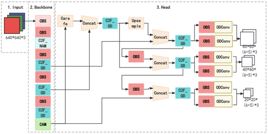
Figure 1.
S-YOLO model structure diagram.
3.1. Replacement of the Convolution Module
In YOLOv8’s native network structure, convolution layers using standard convolution have the following limitations:
- (1)
- Standard convolution can only learn fixed convolution kernels, lacking adaptive adjustment ability for convolution kernel weights, which reduces the convolution layer’s generalization ability and adaptability under different input conditions;
- (2)
- Standard convolution mainly relies on matrix multiplication as operation mode, which results in a large number of parameters and amount of computation, especially in the fully connected layer, which increases the model’s storage and inference overhead;
- (3)
- Standard convolution cannot fully utilize spatial information and channel information of input features, because they use the same weights for each position and each channel, which makes the model ignore some meaningful local features or global features.
To solve the above existing limitation problems, this paper adopted a novel convolution structure, namely, omni-dimensional dynamic convolution (ODConv). ODConv adopts a multi-dimensional attention mechanism [22], which can parallelly allocate dynamic attention weights for the convolution kernel on the four dimensions of kernel space (namely, spatial size of each convolution kernel, input channel number, output channel number, and convolution kernel number). By embedding ODConv into YOLOv8’s network structure, this paper achieves significant improvement of model performance.
ODConv is a dynamic convolution operation that can adaptively adjust convolution kernel weights according to the content of the input feature map. The idea of ODConv is to use an attention mechanism to generate the weight vector for each position and multiply it with shared convolution kernel to obtain the dynamic convolution kernel. ODConv enhances expression ability and adaptability of the convolution layer and improves model performance in scenarios such as small target detection and multi-scale change. Dynamic convolution is different from conventional convolution in that it performs weighted combination of multiple convolution kernels to achieve input relevance. Dynamic convolution’s mathematical expression is as follows:
In the above equation, y is the output feature map, x is the input feature map, is the i-th convolution kernel, is the attention weight of the i-th convolution kernel, * is the convolution operation and n is the number of convolution kernels.
Dynamic convolution’s formula consists of two basic elements: convolution kernel and attention function used to calculate attention weight. For n convolution kernels, the constituted kernel space contains four dimensions: spatial kernel size, input channel number, output channel number, and n. However, CondConv [23] and DyConv [24] only use one attention scalar to calculate the output convolution kernel’s attention weight, while ignoring the spatial dimension, input channel dimension, and output channel dimension of the convolution kernel. CondConv is a type of convolution that learns specialized convolutional kernels for each example by parameterizing the kernels as a linear combination of n experts [23]. DyConv is a type of convolution that dynamically integrates multiple parallel kernels into one dynamic kernel based on the input [24]. It can be seen that CondConv’s and DyConv’s exploration of kernel space is rough. In addition, compared with conventional convolution, dynamic convolution requires n times more convolution kernel parameters (for example, if CondConv , then DyConv ). If dynamic convolution is used too much, it will significantly increase model size. When removing attention mechanism from CondConv/DyConv, their performance improvement is less than 1%. According to these data, it can be concluded that attention mechanism plays a vital role in dynamic convolution: it determines how convolution kernels are generated and how weights are allocated. By improving the attention mechanism’s structure and parameters, a better balance between model accuracy and size can be achieved. ODConv can fully utilize multiple dimensions of kernel space including kernel size, kernel number, and kernel depth, thus making it superior to existing methods such as CondConv and DyConv in terms of model accuracy and size.
In order to achieve ODConv’s four types of attention values, we drew on the idea of CondConv and DyConv and used SE-style attention modules to dynamically generate different types of convolution kernels. Specifically, we first needed to perform global average pooling (GAP) on the input feature map to obtain a feature vector of length C, , and then needed to use a fully connected layer (FC) and four different branches to generate four types of attention values, corresponding to spatial, channel, depth, and angle dimensions. As shown in Figure 2, the structure of these four branches is as follows:
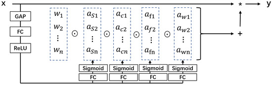
Figure 2.
ODConv structure diagram.
- (1)
- Spatial branch: This branch is used to generate spatial attention values, i.e., weights, for each position. It maps the feature vector to a vector of length , , and then normalizes it using the Softmax activation function. Spatial attention values can be used to adjust the importance of different positions, thereby enhancing the feature expression of regions of interest.
- (2)
- Channel branch: This branch is used to generate channel attention values, i.e., weights for each channel. It maps the feature vector to a vector of length C, , and then normalizes it by the sigmoid activation function. Channel attention values can be used to adjust the contribution of different channels, thereby enhancing the feature expression of semantic relevance.
- (3)
- Depth branch: This branch is used to generate depth attention values, i.e., weights for each convolution kernel group. It maps the feature vector to a vector of length K, , and then normalizes it using the Softmax activation function. Depth attention values can be used to select the most suitable convolution kernel group for the current input, thereby enhancing the feature expression of diversity and adaptability.
- (4)
- Angle branch: This branch is used to generate angle attention values, i.e., weights for each convolution kernel rotation angle. It maps the feature vector to a vector of length R, , and then normalizes it using the Softmax activation function. Angle attention values can be used to select the most suitable convolution kernel rotation angle for the current input direction, thereby enhancing the feature expression of rotation invariance and orientation sensitivity.
Figure 2 depicts the forward propagation process of ODConv, which produces the output feature map based on the input feature map and the convolution kernel parameters. Each node in the calculation diagram corresponds to a variable or operation in the formula, and each edge corresponds to an operator or assignment in the formula. The input feature graph is located at the top-left corner of the diagram, while the output feature graph is at the bottom-right corner. Various intermediate variables and operations are shown in the middle. The calculation diagram consists of three parts:
- (1)
- The first part generates four types of attention values: spatial attention value s, channel attention value c, depth attention value d, and angular attention value . This part corresponds to Equations (2)–(5), where each attention value is computed by applying a fully-connected layer and an activation function to the input feature vector ;
- (2)
- The second part is to generate the dynamic convolution kernel , where each dynamic convolution kernel is obtained by applying depth and angle attention weighting to the convolution kernel parameters ;
- (3)
- The third part is to generate the output feature map , where each output feature map is obtained by spatially and channel-attention weighting the input feature map and then convolving it with the dynamic convolution kernel .
By such design, we can achieve ODConv’s four types of attention values and dynamically generate different types of convolution kernels according to them. ODConv uses attention mechanism on four scales (input channel, output channel, kernel space, and kernel number) to adjust the convolution kernel’s weight and shape. Therefore, it can be described as follows:
In the above equation,
is input channel attention weight:
is a fully connected layer:
is output channel attention weight:
is a fully connected layer:
is kernel space attention weight:
is a fully connected layer:
is kernel number attention weight:
is a fully connected layer:
and is the i-th static convolution kernel.
Based on the property that ODConv can be combined with other optimization techniques, as shown in Figure 3, this paper replaced all standard convolution operations in YOLOv8’s network structure with ODConv operations to enhance the network’s dynamics and adaptability. The specific steps and implementation details were as follows:
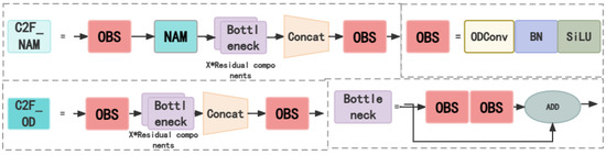
Figure 3.
ODconv replacement module diagram.
- (1)
- In the backbone network, we replaced all convolution layers after the first one, the C2f module and all Conv in the SPPF module with ODConv, but keeping other parameters unchanged;
- (2)
- In Head, we replaced Conv in each detection layer with ODConv, keeping other parameters unchanged;
- (3)
- We trained using the same dataset, evaluation metrics, and experimental environment, and compared and analyzed with the original YOLOv8 model.
Compared with the YOLOv8-nano model, the optimized model—after replacing standard convolution with ODconv—has reduced number of parameters and amount of computation and has improved mAP, recall rate, and precision rate. This shows that the ODconv module has a significant improvement effect on weld defect detection performance. ODconv module’s advantages are mainly reflected in three aspects: first, it reduces model complexity and improves model efficiency and deployability; second, it enhances the model’s detection accuracy and reliability; third, it increases the model’s scale adaptability and robustness. In summary, the ODconv module is an effective improvement method that can improve weld defect detection performance.
3.2. Introduction of the NAM Attention Mechanism
This paper introduces a normalization-based attention module (Normalization-based Attention Module, NAM) to address the YOLOv8 model’s shortcomings in the weld defect detection task, to enhance the model’s feature extraction and classification ability. NAM uses a scaling factor in batch normalization as the channel and spatial attention weight [25], which can adaptively adjust the model’s degree of attention to weld defect features, thereby improving detection accuracy and robustness. At same time, NAM uses sparse regularization to suppress insignificant features, reduce computation overhead, and maintain the model’s efficiency. It can solve the following problems existing in the YOLOv8 model:
- (1)
- YOLOv8 relies on large-scale annotated data to train the model, while weld defect samples in industrial scenarios are often scarce and difficult to collect, which limits the model’s generalization ability and adaptability;
- (2)
- YOLOv8 adopts an Anchor-free detector which directly regresses the target’s position and size. Such a design reduces the number of model parameters, but may also lead to unstable detection results, especially for irregularly shaped and differently sized weld defects;
- (3)
- YOLOv8’s backbone network uses the cross-stage partial connection method to balance network depth and width and improve feature extraction efficiency. However, this method may also cause insufficient information flow between feature maps, affecting capture of weld defect details.
The NAM attention mechanism is a neural network module based on a self-attention mechanism which can adaptively adjust weights of different positions in the feature map, thereby enhancing the expression ability of regions of interest. A self-attention mechanism is a method of calculating the relationship between each element and other elements in the input sequence; it can capture any long-distance dependency relationships in the input sequence, and can calculate these in parallel. The self-attention mechanism can be expressed as
In the above equation [26], Q, K, and V, respectively, represent query (Query), key (Key), and value (Value), and matrix represents key vector dimensions. A self-attention mechanism can be regarded as a weighted average operation based on dot-product similarity, which performs a dot-product operation on a query matrix and a key matrix, normalizes the result into a probability distribution, and then performs a weighted average operation on this probability distribution as weight and value matrix to obtain the output matrix.
The NAM attention mechanism applies a self-attention mechanism to a convolutional neural network and uses a simple and effective integral form to represent attention weight. The NAM attention mechanism can be expressed as
In the above equation, X represents the input feature map and represents the feature vector at the i-th position, and f represents a learnable function such as a fully connected layer or convolution layer. The NAM attention mechanism can be regarded as a weighted average operation based on an exponential function which maps the feature vector at each position in the input feature map to a scalar by a function, exponentiates it to a positive number, normalizes it into a probability distribution, and then performs a weighted average operation on this probability distribution as weight and input feature map to obtain the output feature map.
For model design, this paper adopted the method of adding the NAM attention mechanism to the C2f module to enhance information flow between different channels in the feature map. Specific implementation details are as follows:
- (1)
- Insert the NAM attention mechanism before the last convolution layer in the C2f module, i.e., perform the NAM attention transformation on the feature map output using a convolution layer, and then use the transformed feature map as the convolution layer’s input. This allows the convolution layer to receive more useful channel information and improve the feature map’s expression ability and distinction;
- (2)
- Set the NAM attention mechanism’s parameter to , i.e., divide each channel into four sub-regions and perform a self-attention calculation on each sub-region. This can reduce computation amount and memory consumption while maintaining sufficient receptive field. Use the Softmax function and a convolution layer to implement a self-attention calculation, and use a residual connection and normalization layer to stabilize the training process.
This paper determined, through experimental comparison, that the C2f module in the third layer of the backbone network is the best position to addthe NAM attention mechanism, based on the following reasons:
- (1)
- The third layer of the backbone network provides rich and abstract semantic information suitable for the target detection task. The NAM attention mechanism can utilize the semantic relationship between channels to enhance feature map’s semantic information and improve target detection accuracy and robustness;
- (2)
- The C2f module is a module with multi-hop layer connection and branch structure which can enhance information flow between different scales and positions in the feature map in a suitable way for the multi-scale target detection task. Adding the NAM attention mechanism in this module can utilize the spatial relationship between different channels to enhance the feature map’s spatial information and improve target detection sensitivity and stability;
- (3)
- The NAM attention mechanism can further enhance information flow between channels in the C2f module, improving feature expression ability and target detection performance. The NAM attention mechanism can adaptively adjust weights between channels to highlight useful channel information, suppress useless channel information, and improve the feature map’s diversity and efficiency.
3.3. Replacement of the SPPF Module
The SPPF module is an improvement of spatial pyramid pooling which is used to fuse multi-scale features; it is located at the last layer of the YOLOv8-nano model’s backbone network. It can concatenate features of the same feature map at different scales together to achieve multi-scale feature fusion, improving the feature map’s expression ability and diversity. However, the SPPF module also has the following shortcomings:
- (1)
- It only captures fixed-scale features and cannot adapt to differently sized targets;
- (2)
- Pooling operation reduces feature map spatial resolution, losing detailed information;
- (3)
- The parameter amount is large, increasing computation amount and memory occupancy.
The context augmentation module (CAM) is a module for extracting and fusing context information of different scales, which can effectively utilize information on spatial and channel dimensions, improve feature expression ability and distinction, and enhance context information of the feature pyramid network. The context augmentation module consists of a spatial attention module and a channel attention module, which are used to extract context information on spatial and channel dimensions, respectively, and fuse them into the original feature map. In addition, it uses multiple dilated convolutions with different dilation rates, which are 1, 3, and 5, to obtain context information from different receptive fields and integrate them into the feature pyramid, enriching the semantic information of the feature map, while introducing only a small number of parameters and amount of computation. The context augmentation module is applied to the highest layer of the feature pyramid network to obtain more background information, which is conducive to the detection of tiny defects. The structure of the context augmentation module is shown in Figure 4, where the kernel size of the dilated convolution layer is , and does not change the size of the feature map.
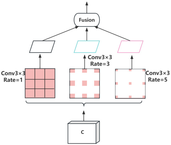
Figure 4.
Context augmentation module structure diagram.
Three different feature fusion methods are considered in the context augmentation module, which correspond to subfigures (a), (b), and (c) in Figure 5. The purpose of these methods is to combine features of different receptive fields to improve detection performance.
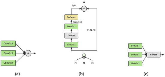
Figure 5.
Feature fusion schematic: (a) Weighted Fusion; (b) Adaptive Fusion; (c) Concatenation Fusion.
This paper compares three different feature fusion methods: (a) weighted addition method, (b) spatial adaptive method, and (c) cascade addition method. The difference between these methods lies in how they combine features of different receptive fields on spatial and channel dimensions. Specifically, assuming that the size of the input feature is (bs, C, H, W), where bs is the batch size, C is the number of channels, and H and W are the height and width, the operations of the three methods are as follows: (a) weighted addition method—directly perform element-wise addition on the input features, resulting in an output feature with a size of (bs, C, H, W); (b) spatial adaptive method—apply a 1 × 1 convolution layer to the input features to compress the number of channels, use a convolution layer to predict the upsampling kernel for each position (which are different for each position), and then use Softmax normalization; the spatial weight matrix with a size of (bs, 3, H, W) is multiplied by the input features aligned by channel to obtain an output feature with a size of (bs, C, H, W); (c) cascade addition method—concatenate the input features on the channel dimension to obtain an output feature with a size of (bs, 3C, H, W).
The purpose of replacing the original SPPF module with the context augmentation module in this paper was to improve the information utilization rate of feature maps on spatial and channel dimensions, thereby enhancing weld defect detection performance. The SPPF module only utilizes spatial dimension information and ignores channel dimension information, resulting in poor feature representation and robustness. The context augmentation module can effectively integrate spatial and channel dimension information to enhance feature expression ability and distinction. Compared with the SPPF module, the context augmentation module has the following advantages:
- (1)
- The context augmentation module can improve the detection effect for difficult-to-detect targets such as small targets, dense targets, occluded targets, etc. The SPPF module uses fixed-size pooling operations which may ignore or lose weld defects that vary greatly, or are small, occluded, or overlapped in scale. The context augmentation module can adaptively select features of different scales and positions and dynamically fuse them to adapt to weld defects of different sizes and shapes;
- (2)
- The context augmentation module can improve generalization ability for diversified datasets with different categories, different scenes, different lighting, etc. The SPPF module uses a max pooling operation, which may ignore or confuse weld defects that vary greatly or are small in category, scene, or lighting. The context augmentation module can enhance features of regions of interest by attention mechanism, suppress features of irrelevant regions, improve feature interpretability and accuracy, and adapt to diversified datasets with different categories, different scenes, different lighting, etc.;
- (3)
- The context augmentation module can improve recognition ability for weld defect position, shape, size, and other detail information. The SPPF module uses concatenation operation, which may cause channel information conflict and confusion, reducing feature diversity and efficiency. The context augmentation module can select more useful channel information by an attention mechanism and fuse it into an original feature map, extracting more fine and meaningful features.
The specific steps of replacing the original SPPF module with the context augmentation module, as performed in this paper, are as follows:
- (1)
- Find the position of the SPPF module in the backbone network of the YOLOv8-nano model, which is after the last convolution layer, and delete it;
- (2)
- Add the context augmentation module to the backbone network of the YOLOv8-nano model, which is inserted after the last convolution layer;
- (3)
- Train with three different feature fusion methods, which arethe weighted addition method, spatial adaptive method, and cascade addition method, and compare them with the original YOLOv8-nano model.
3.4. Introduction of the Carafe Operator
The Upsample operation used by YOLOv8-nano is a traditional interpolation method, which only utilizes spatial information from the input feature map and ignores semantic information. In weld defect detection, this leads to information loss or blur, small receptive field, and low performance. Therefore, this paper introduced the Carafe operator [27], which is a lightweight general upsampling operator that can predict and reorganize upsampling kernels according to input feature map content, thereby improving the upsampling effect. The workflow of Carafe is as follows:
- (1)
- Upsampling kernel prediction: For the input feature map, first use a convolution to compress channel number, then use a convolution to predict the upsampling kernel for each position (which are different for each position), and then use Softmax normalization;
- (2)
- Feature reorganization: For each position in the output feature map, map back to the input feature map, take out a area centered on it, and calculate the dot-product with the predicted upsampling kernel at that point to obtain the output value. Different channels at the same position share the same upsampling kernel.
Carafe has significant advantages over the original Upsample operation. First, Carafe can guide generation of the upsampling kernel according to semantic information of the input feature map, thereby adapting to features of different content and scales, while Upsample is a fixed upsampling method that only determines the upsampling kernel according to pixel distance without utilizing semantic information of the feature map. Second, Carafe can increase receptive field by adjusting convolution, using surrounding information for upsampling to improve upsampling quality, while Upsample has small receptive field (nearest neighbor , bilinear ) and cannot fully utilize surrounding information. Finally, Carafe only introduces a small number of parameters and amount of computation, maintaining lightweight characteristics, while Upsample introduces additional parameters and computation, especially when using deconvolution.
In this paper, we replace the Upsample operation in each layer of the top-down part in YOLOv8 with the Carafe operation; keep other parts unchanged; train with the same dataset, evaluation metric, and experimental environment; and compare and analyze with the original YOLOv8-nano model. Specific steps and implementation details are as follows:
- (1)
- In the Head, we replace the Upsample operation in the first upsampling layer with the Carafe operation for training, and compare and analyze with the original YOLOv8 model.
- (2)
- In the Head, we keep the Upsample operation in the first upsampling layer unchanged, replace the Upsample operation in the second upsampling layer with the Carafe operation for training, and compare and analyze with this YOLOv8-nano model.
- (3)
- In the Head, we replace the Upsample operation in each layer of the top-down part with the Carafe operation for training, and compare and analyze with this YOLOv8 model.
3.5. Optimize Loss Function
This paper studies multi-class weld defect detection, which has a class imbalance problem. Using YOLOv8-nano model’s CIoU loss function, it is easy to cause the model to bias towards multi-sample categories and ignore few-sample categories, affecting detection ability. To solve this problem, this paper chose the Wise-IoU loss function, introduced a category weight coefficient, adjusted target category importance, and balanced the detection effect.
CIoU Loss is a regression error measure used for object detection [28]. It integrates IoU, center distance, and aspect ratio of prediction box and real box, making the model pay more attention to mismatched samples and reducing the loss weight of close samples. CIoU Loss is an improvement of GIoU Loss and DIoU Loss, adding consideration of center point distance and aspect ratio difference. CIoU Loss can improve target detection performance of different scales and shapes, and reduce sensitivity to hyperparameter selection. CIoU Loss’s formula is as follows:
In the above equation, is intersection over union, is Euclidean distance between center points of prediction box and real box, c is diagonal length of smallest closed rectangle containing prediction box and real box, is the balance coefficient, and v is the aspect ratio penalty term. ’s and v’s calculation methods are as follows:
In the above equation, and are prediction box’s and real box’s width and height, respectively.
In the target detection task, the loss function’s design has a decisive role in model performance. An appropriate loss function can enhance boundary box’s fitting accuracy and robustness. However, most existing loss functions are based on an assumption: all samples in training data are high-quality. This assumption ignores the adverse impact of low-quality samples on model performance. To solve this problem, some researchers proposed loss functions based on IoU (intersection over union) to measure overlap degree between prediction box and target box. However, these loss functions have their own limitations and defects. For example, IoU loss [29] cannot provide gradient information when prediction box and target box do not overlap; GIoU loss [29] produces the wrong gradient direction when prediction box contains target box; DIoU loss [30] does not consider whether boundary box’s aspect ratio is consistent; CIoU loss [30] still penalizes distance and aspect ratio difference too much when prediction box and target box overlap a lot; EIoU loss’ [31] assigns too high of a weight to the distance penalty term and uses momentum sliding average value as the unstable normalization factor; and SIoU loss [32] introduces additional penalty terms such as boundary box center line, coordinate axis angle boundary box shape difference, etc. These loss functions do not consider Anchor box’s quality problem, i.e., if low-quality Anchor boxes are excessively regressed, this reduces the model’s localization ability. To overcome these problems, some scholars proposed a loss function based on IoU called Wise-IoU (WIoU) [33]. WIoU uses outlierness to evaluate Anchor box’s quality and adjusts gradient gain dynamically according to outlierness. In this way, WIoU can adaptively select medium-quality Anchor boxes and effectively improve the detector’s overall performance.
WIoU loss function’s definition is as follows:
In the above equation, N is Anchor box’s number, is IoU value between i-th Anchor box and target box, is i-th Anchor box’s corresponding gradient gain, defined as
In the above equation, is i-th Anchor box’s outlierness and is a hyperparameter used to control the gradient gain distribution’s sharpness. Outlierness is an indicator that reflects Anchor box’s quality, defined as
In the above equation, is the length of the center point connection line between i-th Anchor box and target box, and is the diagonal length of the smallest bounding box containing two boundary boxes. Smaller outlierness means higher Anchor box quality.
Wise-IoU and CIoU are both loss functions based on IoU. Their main difference is that Wise-IoU introduces a dynamic non-monotonic focusing coefficient which evaluates Anchor box’s quality by outlierness, adjusts gradient gain of different quality Anchor boxes, and makes the model focus on ordinary quality Anchor boxes. Outlierness is an indicator that integrates IoU and distance measurement; smaller outlierness means higher Anchor box quality. Wise-IoU’s focusing coefficient changes non-monotonically with outlierness; when outlierness is within a certain range, the focusing coefficient is larger, while, when outlierness exceeds this range, the focusing coefficient is smaller. This can reduce the gradient generated by high-quality Anchor boxes and low-quality Anchor boxes, and increase the gradient generated by ordinary-quality Anchor boxes.
As shown in Figure 6, Wise-IoU can replace CIoU in YOLOv8 to achieve better detection performance, which can better handle low-quality examples in the training data, avoid over-penalizing or fitting these examples, and improve the model’s generalization ability and localization accuracy. At the same time, Wise-IoU can better utilize the contextual information of different scales and receptive fields, and allocate reasonable gradient gains through a dynamic non-monotonic focusing mechanism, improving the model’s regression ability for ordinary quality Anchor boxes. Wise-IoU does not introduce additional geometric metrics or computational complexity, but only multiplies a focusing coefficient by the IoU loss, so it can better adapt to different hardware platforms and deployment scenarios.
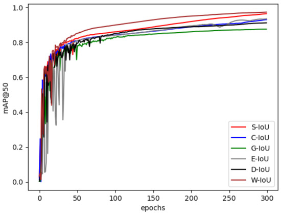
Figure 6.
Effect of different loss functions on model training.
4. Experimental Verification and Analysis
4.1. Dataset
The detection target of this paper was weld defects, and, for the convenience of data processing, this paper set the format of weld defect images used to make the dataset as the PASCALVOC2007 format.
4.1.1. Weld Defect Image Augmentation
The deep learning-based weld detection algorithm is a task that uses deep neural networks to identify and locate welding defects, which requires a dataset of normal and abnormal weld images, along with their defect feature images. However, insufficient annotation of datasets is a difficult problem, which leads to the following:
- (1)
- The network learns defect features and rules insufficiently, resulting in low detection performance and accuracy;
- (2)
- The dataset is unbalanced, with a disproportionate ratio of normal and abnormal weld images, resulting in low detection sensitivity and recall;
- (3)
- The dataset is not representative, unable to cover the diversity and complexity of weld defects, resulting in low detection robustness and adaptability.
To solve this problem, a possible method is to use cross-modal data transfer to make weld defect datasets. Cross-modal data transfer [34,35,36] has two types of methods: feature-based and image-based. This paper uses feature-based cross-modal data transfer to make weld defect datasets, with the following steps:
- (1)
- Collect or obtain weld images with or without annotations from different imaging modalities;
- (2)
- Extract representative and discriminative features from the images;
- (3)
- Align or transform features to make them similar or consistent in a common feature space;
- (4)
- Train classifiers or segmenters to detect weld defects.
In order to preserve defect feature information and unify resolution, this paper used a region-of-interest segmentation method. This method is a region-based image segmentation method that divides an image into several regions with similar features and extracts the regions of interest. The regions of interest are usually parts of an image that contain target objects or information, such as the location and shape of weld defects. This paper performed region of interest segmentation on weld defect images to highlight defect features and eliminate background interference.
This paper constructed a weld defect detection dataset using two sources of image data: a weld defect image dataset from a factory (4652 images of different types of weld defects, unbalanced in quantity) and the Northeastern University steel strip surface defect image dataset (1800 images of six types of steel strip surface defects, namely, rolled-in scale, patches, crazing, pitted surface, inclusion, and scratches, with a resolution of ). This paper considered that the defect types in the two datasets were similar and general, and constructed a more complete dataset by processing and augmenting them. This paper performed the following steps on the two datasets:
- (1)
- In view of the problem of low quality of ultrasonic images of weld defects, this paper proposed an image enhancement method based on the multi-scale retinex algorithm. This method first uses an anisotropic diffusion algorithm to denoise, then uses histogram equalization processing to improve contrast, and, finally, applies the multi-scale retinex algorithm to boththe original image and equalized image, obtaining enhancement results by weighted fusion. This method effectively improves the quality of ultrasonic images of weld defects, providing reliable data support for subsequent detection and identification;
- (2)
- In order to unify the image size and format of the two datasets, this paper set the resolution to . For weld defect images from the factory, since they have high resolution and uneven distribution of defect areas, direct scaling would result in loss or distortion of defect information. Therefore, this paper adopted a cropping method based on region of interest (ROI). Specifically, this paper used the ROI function in the openCV library, which selects ROI by clicking on the image with mouse and returning coordinates. Then, according to the coordinates, it crops out sub-images containing defect information. This not only meets the requirement of uniform size, but also retains the original defect features;
- (3)
- In order to increase the number and diversity of dataset samples, this paper performed data augmentation on the two datasets. This paper used data augmentation methods such as horizontal flipping, vertical flipping, rotation, translation, random cropping, etc. These methods increase the variation and noise of the dataset without changing the defect type and feature, thereby improving the model’s generalization ability and robustness. Through data augmentation, this paper, finally, obtained a dataset containing 20,800 images, with each image category containing more than 3000 samples, as shown in Figure 7.
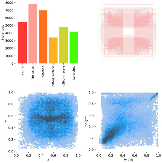 Figure 7. Distribution of dataset labels and target boxes.
4.1.2. Welding Defect Dataset Production
In this paper, we chose the AnyLabeling tool, based on Segment Anything as shown in Figure 8, for annotation work. Segment Anything is an image segmentation method that can segment any object in an image according to different input prompts (such as points, boxes, text, etc.), and can generalize to unfamiliar objects and images in a zero-shot manner without additional training. The basic principle of Segment Anything is to use a neural network model to encode the input prompts and images into a feature vector, and then generate a segmentation mask through a decoder.
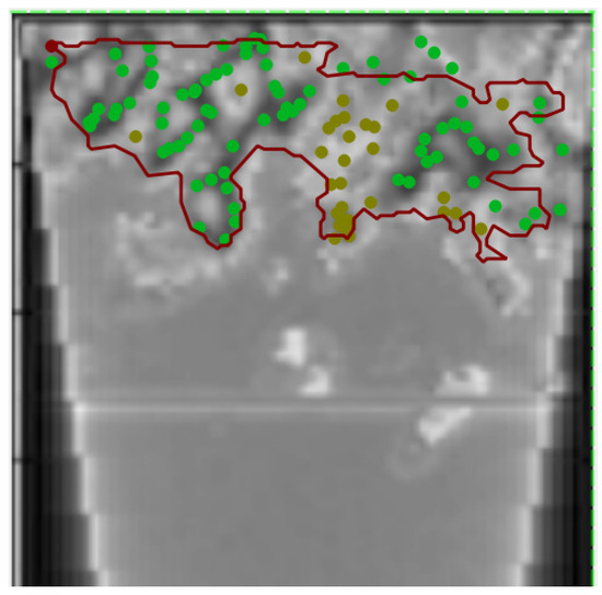
Figure 8.
Labeling process with AnyLabeling.
In order to evaluate the impact of the annotation method and data augmentation method used in this paper on the defect detection model performance, we used the original annotated dataset as the control group, and compared it with the dataset annotated by the method proposed in this paper as the experimental group. The dataset used in this paper was in VOC2007 format, which consisted of three folders: ImageSets folder which stores txt files for dividing the training set, validation set and test set; JPEGImages folder which stores all image data; Aand nnotations folder which stores all XML annotation files of images. The dataset is divided into training set, validation set, and test set according to the ratio of 8:1:1. In order to construct a dataset suitable for the method proposed in this paper and enhance the generalization ability of the model, we performed various data augmentation operations on the training set, including flipping, scaling, cropping, color transformation, etc. The experimental results show that the model trained with the supplemented dataset achieved 97.3% accuracy, 95.6% recall, and 94% F1 value on the test set, which were 2.3%, 3.1%, and 2.5% higher than those of the control group, respectively, demonstrating a significant improvement in the model’s defect detection ability.
4.2. Experimental Environment and Scheme Design
In order to ensure the training effect and stability of the model, we chose suitable hardware and software configuration as the experimental environment. The specific environment information is shown in Table 1.

Table 1.
Experimental environment configuration table.
Before training, we divided the VOC format dataset into training set, validation set, and test set, according to the ratio of 8:1:1, where each image size was pixels. The training set was used for model training and parameter updating, the validation set was used for model tuning and hyperparameter selection, and the test set was used for model evaluation and performance comparison. In order to train the model, we used stochastic gradient descent (SGD) as the optimizer and set the training batch size to 128, initial learning rate to 0.01, and model iteration number to 300. In order to prevent overfitting, we added a momentum term and weight decay term in the optimizer, which were set to 0.9 and 0.0005, respectively. In order to adapt to the learning rate change during the training process, we useda cosine annealing strategy as the learning rate decay strategy to dynamically adjust learning rate according to training rounds. These parameter settings aimed to ensure model convergence and generalization.
4.3. Evaluation Metrics
In this paper, we mainly used two metrics commonly used for evaluating object detection model performance: mean average precision (mAP) and frames per second (FPS), to comprehensively evaluate and analyze the model performance. In addition, we also introduced factors, such as parameter quantity, from a side perspective to analyze algorithm effect.
FPS is the number of pictures that the object detection model can process per second; it reflects model detection speed. A higher FPS means that the model is faster. The FPS calculation method is
In the above equation, is total processing time; is preprocessing time; is detection time; and is post-processing time.
Mean average precision mAP is an indicator that measures object detection model performance; it is the average value of average precision (AP) of all categories. AP is the average value of precision corresponding to different recall rates (recall). The mAP derivation formula is as follows:
Precision P:
The Precision (P) formula indicates, among samples predicted as positive examples, the proportion which are true positive examples. TP is the number of true positive examples, indicating the number of samples that are predicted as positive examples and are actually positive examples. FP is the number of false positive examples, indicating the number of samples that are predicted as positive examples but are actually negative examples. TP + FP is the number of all samples predicted as positive examples. Thus, P = TP/(TP + FP) is the proportion of true positive examples out of the total number of examples predicted as positive examples.
Recall rate R:
The Recall rate (R) formula indicates, among original samples of positive examples, the proportion which are correctly predicted. TP is the number of true positive examples, indicating the number of samples that are predicted as positive examples and are actually positive examples. FN is the number of false negative examples, indicating the number of samples that are predicted as negative examples but are actually positive examples. TP + FN is the number of all true positive examples. Thus, R = TP/(TP + FN) is the proportion of correctly predicted positive examples out of the total number of predicted positive examples.
AP value:
The AP value formula indicates the average value of precision corresponding to different recall rates. P(k) is the value of precision corresponding to the k-th recall rate; R(k) is the k-th recall rate. R(k) indicates the difference between the k-th recall rate and the (k − 1)-th recall rate. AP value is the sum of all different recall rates multiplied by the corresponding difference, which is equivalent to calculating the area under the PR curve.
Average AP value:
In the above equation, m is the number of categories and AP is the AP value of the i-th category. The average AP value formula indicates that, for prediction results from multiple categories, the AP value of each category is calculated and then the average is taken. Since AP is the AP value of the i-th category and m is the number of categories, average AP value is the sum of all category AP values divided by the number of categories.
FPS is an indicator that measures model speed; it has a certain balance and trade-off relationship with model accuracy indicators (such as mAP). Therefore, we need to comprehensively consider FPS and mAP, analyze model advantages and disadvantages in terms of speed and accuracy, and select the most suitable model.
4.4. Experimental Results Analysis
In the industrial application scenario of this paper, we needed to detect and evaluate welding defects. The experiment in this paper was trained on a dataset containing 20,800 welding images, which included 6 common types of defects (scratches, oxide skin, indentations, iron oxide skin, edge defects, other defects). We conducted performance evaluations on the S-YOLO model through five groups of experiments, where the first group was a comparative experiment on the impact of different convolutions on model performance; the second group was a comparative experiment on the impact of different attention mechanisms on model performance; the third group was a performance comparison experiment on different fusion methods of the context augmentation module; the fourth group was an ablation experiment on improvement strategies in the S-YOLO model; and the fifth group was a comprehensive analysis of model performance by comparing S-YOLO with current mainstream object detection models.
In order to verify the proposed welding defect detection algorithm and its effectiveness, we monitored the change curves of three loss functions during the training process, as shown in Figure 9. In Figure 9a, Box Loss represents the mean value of the loss function for bounding box regression, which uses Wise-IoU as the bounding box loss function, which can dynamically allocate gradient gain according to the overlap degree between Anchor boxes and target boxes and improve the accuracy of bounding box regression. In Figure 9b, Classification Loss represents the mean value of the loss function for target classification, which reflects the classifier’s ability to recognize target categories. In Figure 9c, Distribution Focal Loss represents the distributional focal loss, which is a loss function for addressing the class imbalance problem in object detection, which can reduce the contribution of simple samples to the loss value and make the model better learn difficult samples. As can be seen from Figure 9, in the first 20 rounds, the three loss values decreased significantly, indicating that the model had a large learning progress in the initial stage; between 20 and 120 rounds, Box Loss showed an upward trend, while Classification Loss and Distribution Focal Loss decreased steadily, which was due to the model encountering difficult-to-fit bounding boxes at this stage; between 120 and 290 rounds, Box Loss gradually decreased, while Classification Loss and Distribution Focal Loss decreased at a slower rate, which may be due to the model gradually adapting to the data distribution at this stage; after 290 rounds, the data augmentation strategy was turned off, and all three loss values decreased significantly, indicating that the data augmentation strategy could effectively improve the model’s generalization ability. No obvious overfitting phenomenon was found in the whole training process.
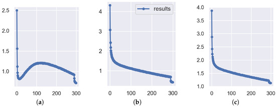
Figure 9.
Loss curve: (a) Box Loss; (b) Classification Loss; (c) Distribution Focal Loss.
4.4.1. The Impact of Different Convolutions on Model Performance
In order to verify the effect of replacing conventional convolution with ODConv, we replaced all standard convolution operations in the YOLOv8-nano model with CondConv [23], DyConv [37], and ODConv on the basis of the YOLOv8-nano model, keeping other parameters unchanged, and obtained three optimized models: YOLOv8-nano-CondConv, YOLOv8-nano-DyConv, and YOLOv8-nano-ODConv. Then, we used the same dataset, evaluation metrics and experimental environment for training and testing, and compared and analyzed with the original YOLOv8-nano model.
As can be seen from Table 2, compared with the YOLOv8-nano model, the optimized model using ODConv also had an improvement in FPS, which indicates that ODConv can speed up model inference speed and improve model detection efficiency. Among them, the YOLOv8-nano-ODConv model had the highest FPS, reaching 69.9, which was 3.2 higher than YOLOv8-nano model. This shows that the ODConv module can effectively reduce model computation and inference time, and achieve a balance between model accuracy and speed.
Table 2.
Comparison results of different convolutions on model performance.
4.4.2. The Impact of Different Attention Mechanisms on Model Performance
In order to verify the effect of introducing the NAM attention mechanism, we introduced SE, CBAM, BiFormer, and NAM attention mechanisms at the same position in the YOLOv8-nano model on the basis of the YOLOv8-nano model, keeping other parameters unchanged, and obtained four optimized models: YOLOv8-nano-SE, YOLOv8-nano-CBAM, YOLOv8-nano-BiFormer, and YOLOv8-nano-NAM. Then, we used the same dataset, evaluation metrics, and experimental environment for training and testing, and compared and analyzed with the original YOLOv8-nano model.
As can be seen from Table 3, the models using attention mechanisms were better than the baseline model in mAP@50, indicating that attention mechanisms can effectively improve the expressiveness and discriminability of feature maps, and enhance the performance of the welding defect detection task. Among them, YOLOv8-nano-BiFormer achieved the highest mAP@50 of 92.1%, which was 3.7% higher than the baseline model, indicating that BiFormer can better utilize the information in spatial and channel dimensions, and improve the semantic and diversity of features. In addition, the models using attention mechanisms were worse than the baseline model in FLOPs and FPS, indicating that attention mechanisms increase the number of model parameters and computation, and affect model efficiency and speed. Among them, YOLOv8-nano-BiFormer had the highest FLOPs, of 10.2 G, which was 1.3G higher than the baseline model, and had the lowest FPS of 61.6, which was 5.1 lower than the baseline model. This indicates that BiFormer can improve detection accuracy, but also pays a large price in the training process; because it needs to occupy a large amount of memory for calculation, its training time is far greater than other attention mechanisms. The NAM attention introduced in this paper achieves 91.0% in mAP@50, second only to the YOLOv8-nano-BiFormer, but has only 9.0G in FLOPs, which is 1.2G lower than the YOLOv8-nano-BiFormer, and achieves 65.8 in FPS, which is 4.2 higher than YOLOv8-nano-BiFormer, indicating that YOLOv8-nano-NAM can ensure detection accuracy while also maintaining high efficiency and speed.
Table 3.
The effect of different attention mechanisms on the performance of the YOLOv8-nano model.
4.4.3. Performance Comparison of Different Fusion Methods in the Context Augmentation Module
In order to verify the effect of using the spatial adaptive method in the context augmentation module in this paper, we selected the weighted addition method, spatial adaptive method, and cascade addition method as the context augmentation modules applied to the YOLOv8-nano model in this paper, keeping other parameters unchanged. Then, we used the same dataset, evaluation metrics, and experimental environment for training and testing, and conducted comparative experiments and analysis.
As can be seen from Table 4, the YOLOv8 model using the spatial adaptive method achieved the highest mAP@50 of 90.6%, which was 1.7% higher than the weighted addition method and 0.1% lower than the cascade addition method; it achieved the lowest FLOPs of 10.3G, which was 0.2G higher than the weighted addition method and 2.1G lower than the cascade addition method; it achieved the highest FPS of 62.9, which was 0.4 higher than the weighted addition method and 4.3 higher than the cascade addition method. This indicates that the spatial adaptive method can maintain high detection accuracy while also maintaining high efficiency and speed.
Table 4.
Performance comparison results of three feature fusion methods.
4.4.4. The Impact of Improvement Methods on Model Performance and Efficiency
In order to verify the impact of improvement strategies on model performance and efficiency, we used the ablation experiment method for analysis, and took the S-YOLO model with all improvement strategies applied as the baseline model. By gradually removing a certain module or mechanism from the model, we observed its impact on model performance and judged its role in overall model; experimental results are shown in Table 5.
Table 5.
Impact of different improvement strategies on the performance of the S-YOLO model.
Experiment 1: We used the S-YOLO model as the complete improved version, which was also the baseline model. This model achieved 97.3% mAP@50 on the experimental dataset, indicating that it has high detection accuracy. The model had a computation of 8.6G FLOPs and a running speed of 67.8 FPS, indicating that it has high efficiency and speed.
Experiment 2: We replaced the Carafe module in the S-YOLO model with the original nn.Upsample module to explore the effect of the Carafe module on feature map upsampling. The mAP@50 of this model decreased by 0.6 percentage points to 96.7%. At the same time, the FLOPs of this model decreased by 0.1G to 8.5G, and FPS increased by 1.8 to 89.6. The experimental results show that the Carafe module can effectively improve the resolution and quality of feature maps, thereby improving detection accuracy, but its impact on computation and speed is not significant.
Experiment 3: We replaced the context augmentation module in the S-YOLO model with the SPPF module to explore the effect of the context augmentation module on feature fusion. The mAP@50 of this model decreased by 2.8 percentage points to 94.5%. At the same time, the FLOPs of this model decreased by 1.5G to 7.1G and FPS increased by 5.6 to 74.4. The experimental results show that the context augmentation module can effectively improve the correlation and consistency between features, thereby improving detection accuracy, but at the cost of increased computation.
Experiment 4: We replaced ODConv in the S-YOLO model back to Conv to explore the effect of ODConv on feature extraction. The mAP@50 of this model decreased by 4.9 percentage points to 92.4%. At the same time, the FLOPs of this model decreased by 0.4G to 8.2G and FPS increased by 2.9 to 71.7. The experimental results show that ODConv can effectively improve the sparsity and diversity of feature maps, thereby improving detection accuracy, and can also optimize computation and speed to some extent.
Experiment 5: We removed the NAM attention mechanism added in the S-YOLO model to explore the effect of the NAM attention mechanism on feature selection. The mAP@50 of this model decreased by 7.5 percentage points to 89.8%. At the same time, FLOPs decreased by 0.3G to 8.3G and FPS increased by 2.0 to 69.8. The experimental results show that the NAM attention mechanism can effectively improve saliency and discriminability of features, thereby improving detection accuracy.
Experiment 6: We replaced Wise-IoU in the S-YOLO model with CIoU to explore the effect of Wise-IoU on the loss function and optimization process. At this time, the model was also the prototype structure of YOLOv8-nano. The mAP@50 of this model decreased by 8.9 percentage points to 88.4%. At the same time, FLOPs increased by 0.3G to 8.9G and FPS decreased by 1.1 FPS to 66 FPS. The experimental results show that Wise-IoU can effectively improve robustness and stability of the loss function and optimization process.
The S-YOLO object detection model proposed in this paper surpassed the original model in both accuracy and speed. Meanwhile, we also explored the effect of each component of the S-YOLO model on detection performance, loss function, and optimization process. The experimental results show that these components can improve resolution, quality, sparsity, and diversity of feature maps, as well as correlation, consistency, saliency, and discriminability between features, thereby enhancing small object detection ability.
Figure 10 shows the precision–recall (PR) curve of different defect categories for the S-YOLO model. The PR curves indicate the trade-off between precision and recall for different confidence thresholds. A higher area under the curve (AUC) implies a better performance of the model. Figure 10 reveals that the S-YOLO model achieved high AUC values for all defect categories, indicating its high accuracy in detecting and classifying various types of weld defects.
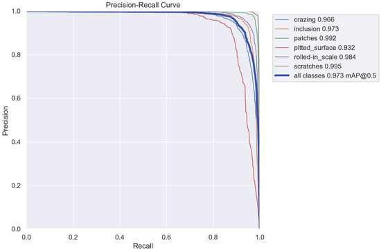
Figure 10.
S-YOLO model PR curve.
Figure 11 presents a example of weld image recognition results for the S-YOLO model and the YOLOv8-nano model. The figure shows the original weld images and the detection results of the two models. Figure 11 shows that the S-YOLO model can accurately detect and label all the defects in the weld images, while the YOLOv8-nano model fails to detect some defects or produces false positives/negatives. This example shows that the S-YOLO model has a higher accuracy and robustness than the YOLOv8-nano model in recognizing weld defects.
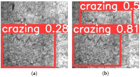
Figure 11.
Comparison of prediction results before and after model improvement: (a) YOLOv8-nano prediction results; (b) S-YOLO forecast results.
4.4.5. Performance Comparison of Different Object Detection Models
In order to evaluate the performance of the S-YOLO algorithm, we compared it with seven other object detection algorithms, and tested them on two indicators: mAP and FPS. The final test results are shown in Table 6.
Table 6.
Impact of different improvement strategies on the performance of the S-YOLO model.
As can be seen from Table 6, the S-YOLO algorithm proposed in this paper was better than other algorithms in both mAP and FPS indicators, indicating that it has efficient and accurate object detection ability. This shows that the S-YOLO algorithm not only retains the speed advantage of the YOLO series, but also improves the detection accuracy for small objects. This table shows the excellent performance of the S-YOLO algorithm in object detection tasks, proving its applicability and effectiveness in experimental scenario.
5. Conclusions
In this paper, we propose an improved model based on the YOLOv8-nano for welding defect detection tasks, namely, the S-YOLO model. This model optimizes and improves various aspects based on the original model structure, including optimizing convolution layer structure, introducing the Carafe operator, replacing the SPPF module, introducing the NAM attention mechanism, optimizing the loss function, etc., to improve model detection accuracy and speed. We used the self-made welding defect dataset for experimental verification and analysis; used mAP, FPS, and other indicators to evaluate algorithm performance; and compared with other object detection models. The experimental results show that the S-YOLO algorithm significantly improves detection accuracy while maintaining high detection speed, achieving good results.
The next step of the work is to optimize the S-YOLO model for lightweighting, ensuring detection performance while reducing model parameter and computation. This will further improve efficiency of welding defect detection, realize real-time processing and output of welding images, synchronize with automated welding processes, and achieve effective welding inspection integration.
Author Contributions
Conceptualization, Q.N. and Y.Z.; methodology, Y.Z.; software, Y.Z.; validation, Y.Z.; formal analysis, Y.Z.; writing—original draft preparation, Y.Z.; writing—review and editing, Q.N. and Y.Z.; visualization, Y.Z.; supervision, Q.N.; project administration, Q.N. and Y.Z.; funding acquisition, Q.N. All authors have read and agreed to the published version of the manuscript.
Funding
This paper is supported by the National Natural Science Foundation of China (12273003).
Data Availability Statement
The data presented in this study are available on request from the corresponding author.
Acknowledgments
The authors wish to thank the reviewers for their careful, unbiased, and constructive suggestions, which led to this revised manuscript.
Conflicts of Interest
The authors declare no conflict of interest.
References
- Stoean, C.; Zivkovic, M.; Bozovic, A.; Bacanin, N.; Strulak-Wójcikiewicz, R.; Antonijevic, M.; Stoean, R. Metaheuristic-Based Hyperparameter Tuning for Recurrent Deep Learning: Application to the Prediction of Solar Energy Generation. Axioms 2023, 12, 266. [Google Scholar] [CrossRef]
- Dang, D.T.; Wang, J.W. Developing a Deep Learning-Based Defect Detection System for Ski Goggles Lenses. Axioms 2023, 12, 386. [Google Scholar] [CrossRef]
- Zhang, Y.; Jiang, H.; Ye, T.; Juhas, M. Deep Learning for Imaging and Detection of Microorganisms. Trends Microbiol. 2021, 29, 569–572. [Google Scholar] [CrossRef] [PubMed]
- Krizhevsky, A.; Sutskever, I.; Hinton, G.E. ImageNet classification with deep convolutional neural networks. Commun. ACM 2017, 60, 84–90. [Google Scholar] [CrossRef]
- Dai, J.; Li, Y.; He, K.; Sun, J. R-FCN: Object detection via region-based fully convolutional networks. In Proceedings of the Advances in Neural Information Processing Systems, Barcelona, Spain, 5–10 December 2016; pp. 379–387. [Google Scholar]
- Ren, S.; He, K.; Girshick, R.; Sun, J. Faster R-CNN: Towards real-time object detection with region proposal networks. IEEE Trans. Pattern Anal. Mach. Intell. 2017, 39, 1137–1149. [Google Scholar] [CrossRef]
- Girshick, R. Fast R-CNN. In Proceedings of the IEEE International Conference on Computer Vision, Santiago, Chile, 7–13 December 2015; pp. 1440–1448. [Google Scholar]
- Redmon, J.; Divvala, S.; Girshick, R.; Farhadi, A. You only look once: Unified, real-time object detection. In Proceedings of the IEEE Conference on Computer Vision and Pattern Recognition, Las Vegas, NV, USA, 27–30 June 2016; pp. 779–788. [Google Scholar]
- He, K.; Gkioxari, G.; Doll’ar, P.; Girshick, R. Mask R-CNN. In Proceedings of the IEEE International Conference on Computer Vision, Venice, Italy, 22–29 October 2017; pp. 2961–2969. [Google Scholar]
- Law, H.; Deng, J. CornerNet: Detecting Objects as Paired Keypoints. Int. J. Comput. Vis. 2020, 128, 642–656. [Google Scholar] [CrossRef]
- Redmon, J.; Farhadi, A. YOLO9000: Better, faster, stronger. IEEE Trans. Pattern Anal. Mach. Intell. 2017, 39, 2119–2129. [Google Scholar]
- Redmon, J.; Farhadi, A. YOLOv3: An Incremental Improvement. arXiv 2018, arXiv:1804.02767. [Google Scholar]
- Wang, C.Y.; Bochkovskiy, A.; Liao, H.Y.M. Scaled-YOLOv4: Scaling Cross Stage Partial Network. In Proceedings of the 2021 IEEE/CVF Conference on Computer Vision and Pattern Recognition (CVPR), Nashville, TN, USA, 20–25 June 2021; pp. 13024–13033. [Google Scholar]
- Karthi, M.; Muthulakshmi, V.; Priscilla, R.; Infantia C, N.; Vanisri, K. Evolution of YOLO-V5 Algorithm for Object Detection: Automated Detection of Library Books and Performace validation of Dataset. In Proceedings of the 2021 International Conference on Innovative Computing, Intelligent Communication and Smart Electrical Systems (ICSES), Chennai, India, 24–25 September 2021; pp. 1–6. [Google Scholar]
- Terven, J.; Cordova-Esparza, D.M. A Comprehensive Review of YOLO: From YOLOv1 and Beyond. arXiv 2023, arXiv:2304.00501. [Google Scholar]
- Reis, D.; Kupec, J.; Hong, J.; Daoudi, A. Real-Time Flying Object Detection with YOLOv8. arXiv 2023, arXiv:2305.09972. [Google Scholar]
- Wang, C.Y.; Bochkovskiy, A.; Liao, H.Y.M. YOLOv7: Trainable Bag-of-Freebies Sets New State-of-the-Art for Real-Time Object Detectors. In Proceedings of the IEEE/CVF Conference on Computer Vision and Pattern Recognition (CVPR), Vancouver, BC, Canada, 18–22 June 2023; pp. 7464–7475. [Google Scholar]
- Li, C.; Li, L.; Jiang, H.; Weng, K.; Geng, Y.; Li, L.; Ke, Z.; Li, Q.; Cheng, M.; Nie, W.; et al. YOLOv6: A Single-Stage Object Detection Framework for Industrial Applications. arXiv 2022, arXiv:2209.02976. [Google Scholar]
- Jawaharlalnehru, A.; Sambandham, T.; Sekar, V.; Ravikumar, D.; Loganathan, V.; Kannadasan, R.; Khan, A.A.; Wechtaisong, C.; Haq, M.A.; Alhussen, A.; et al. Target Object Detection from Unmanned Aerial Vehicle (UAV) Images Based on Improved YOLO Algorithm. Electronics 2022, 11, 2343. [Google Scholar] [CrossRef]
- Haq, M.A. CNN Based Automated Weed Detection System Using UAV Imagery. Comput. Syst. Sci. Eng. 2022, 42, 837–849. [Google Scholar]
- Wang, C.Y.; Liao, H.Y.M.; Yeh, I.H.; Wu, Y.H.; Chen, P.Y.; Hsieh, J.W. CSPNet: A New Backbone that can Enhance Learning Capability of CNN. arXiv 2019, arXiv:1911.11929. [Google Scholar]
- Li, C.; Zhou, A.; Yao, A. Omni-Dimensional Dynamic Convolution. arXiv 2022, arXiv:2209.07947. [Google Scholar]
- Yang, B.; Bender, G.; Le, Q.V.; Ngiam, J. CondConv: Conditionally Parameterized Convolutions for Efficient Inference. In Proceedings of the Advances in Neural Information Processing Systems, Vancouver, BC, Canada, 8–14 December 2019; pp. 1307–1318. [Google Scholar]
- Chen, Y.; Dai, X.; Liu, M.; Chen, D.; Yuan, L.; Liu, Z. Dynamic convolution: Attention over convolution kernels. In Proceedings of the 2020 IEEE/CVF Conference on Computer Vision and Pattern Recognition (CVPR), Seattle, WA, USA, 13–19 June 2020; pp. 11956–11964. [Google Scholar]
- Liu, Y.; Shao, Z.; Teng, Y.; Hoffmann, N. NAM: Normalization-based Attention Module. arXiv 2021, arXiv:2111.12419. [Google Scholar]
- Vaswani, A.; Shazeer, N.; Parmar, N.; Uszkoreit, J.; Jones, L.; Gomez, A.N.; Kaiser, L.; Polosukhin, I. Attention is all you need. In Proceedings of the Advances in Neural Information Processing Systems, Long Beach, CA, USA, 4–9 December 2017; pp. 5998–6008. [Google Scholar]
- Wang, J.; Chen, K.; Xu, R.; Liu, Z.; Loy, C.C.; Lin, D. CARAFE: Content-Aware ReAssembly of FEatures. In Proceedings of the 2019 IEEE/CVF International Conference on Computer Vision (ICCV), Seoul, Republic of Korea, 7 October–2 November 2019; pp. 303–312. [Google Scholar]
- Zhou, D.; Fang, J.; Song, X.; Guan, C.; Yin, J.; Dai, Y.; Yang, R. Complete IoU Loss for Oriented Object Detection. arXiv 2020, arXiv:2007.09584. [Google Scholar]
- Rezatofighi, H.; Tsoi, N.; Gwak, J.; Sadeghian, A.; Reid, I.; Savarese, S. In Proceedings of the 2019 IEEE/CVF Conference on Computer Vision and Pattern Recognition (CVPR), Long Beach, CA, USA, 15–20 June 2019.
- Zheng, Z.; Wang, P.; Liu, W.; Li, J.; Ye, R.; Ren, D. Distance-IoU Loss: Faster and Better Learning for Bounding Box Regression. In Proceedings of the AAAI Conference on Artificial Intelligence, New York, NY, USA, 7–12 February 2020; Volume 34, pp. 12993–13000. [Google Scholar]
- Zhang, Y.F.; Ren, W.; Zhang, Z.; Jia, Z.; Wang, L.; Tan, T. Focal and efficient IOU loss for accurate bounding box regression. Neurocomputing 2022, 506, 146–157. [Google Scholar] [CrossRef]
- Gevorgyan, Z. SIoU Loss: More Powerful Learning for Bounding Box Regression. arXiv 2022, arXiv:2205.12577. [Google Scholar]
- Tong, Z.; Chen, Y.; Xu, Z.; Yu, R. Wise-IoU: Bounding Box Regression Loss with Dynamic Focusing Mechanism. arXiv 2023, arXiv:2301.10051. [Google Scholar]
- Zhang, C.; Yang, Z.; He, X.; Deng, L. Multimodal Intelligence: Representation Learning, Information Fusion, and Applications. IEEE J. Sel. Top. Signal Process. 2020, 14, 478–493. [Google Scholar] [CrossRef]
- Zhen, L.; Hu, P.; Peng, X.; Goh, R.S.M.; Zhou, J.T. Deep Multimodal Transfer Learning for Cross-Modal Retrieval. IEEE Trans. Neural Netw. Learn. Syst. 2022, 33, 798–810. [Google Scholar] [CrossRef] [PubMed]
- Huang, X.; Peng, Y.; Yuan, M. MHTN: Modal-adversarial Hybrid Transfer Network for Cross-modal Retrieval. IEEE Trans. Cybern. 2018, 50, 1047–1059. [Google Scholar] [CrossRef]
- Zhou, J.; Jampani, V.; Pi, Z.; Liu, Q.; Yang, M.H. Decoupled Dynamic Filter Networks. arXiv 2021, arXiv:2104.14107. [Google Scholar]


Disclaimer/Publisher’s Note: The statements, opinions and data contained in all publications are solely those of the individual author(s) and contributor(s) and not of MDPI and/or the editor(s). MDPI and/or the editor(s) disclaim responsibility for any injury to people or property resulting from any ideas, methods, instructions or products referred to in the content. |
© 2023 by the authors. Licensee MDPI, Basel, Switzerland. This article is an open access article distributed under the terms and conditions of the Creative Commons Attribution (CC BY) license (https://creativecommons.org/licenses/by/4.0/).