Abstract
The last few decades have witnessed advancements in intelligent metaheuristic approaches and system reliability optimization. The huge progress in metaheuristic approaches can be viewed as the main motivator behind further refinement in the system reliability optimization process. Researchers have intensively studied system reliability optimization problems (SROPs) to obtain the optimal system design with several constraints in order to optimize the overall system reliability. This article proposes a modified wild horse optimizer (MWHO) for SROPs and investigates the reliability allocation of two complex SROPs, namely, complex bridge system (CBS) and life support system in space capsule (LSSSC), with the help of the same process. The effectiveness of this framework based on MWHO is demonstrated by comparing the results obtained with the results available in the literature. The proposed MWHO algorithm shows better efficiency, as it provides superior solutions to SROPs.
1. Introduction
The crucial role of reliability optimization in 21st century industry is the reason for the extensive involvement of various researchers, industry experts and decision makers (DM) in it. All stakeholders, ranging from automobile industries, transportation systems, and the military to food industries, have some stake in this concept’s success, as the combination of reliability and the associated cost of their products has a significant influence on customer satisfaction. Thus, to remain competitive in today’s world, the basic goal of associated reliability engineers is to improve the overall reliability of the product and its components, as well as maintaining production of the product at a competitive cost [1]. Reliability can be viewed as the probability that a system works uninterrupted for a specific period of time. Reliability is also defined as the probability that a product, system, or service will perform its intended function adequately for a specified period of time, or at least operate in a defined environment without failure [2,3,4]. This definition encourages system engineers to develop a reliable and cost-effective product, which, in turn, increases the complexities and creates a complex system design process and, hence, a complex SROP. Generally, SROPs can be distinguished into three classes, namely, reliability allocation problems (ReAP), redundancy allocation problems (RAP) and reliability–redundancy allocation problems (RRAP) [5]. In all of these approaches, researchers aim to achieve optimal system reliability and cost under certain constraints based on available resources.
The computational complexity associated with SROPs has prompted researchers to solve these problems using the various approaches available in the literature. These approaches can be broadly categorized into two categories, namely, heuristic approaches and metaheuristic approaches [6]. Metaheuristic approaches have an edge over heuristics, as they have a derivative-free mechanism and are quite simple and flexible, even when dealing with highly complex non-linear optimization problems like SROPs. Metaheuristics also have a superior ability to avoid local extrema. SROPs have been proven to be NP-hard in nature, and their computational complexity increases dramatically as the scale of system configuration increases [7,8]. According to the ‘‘No Free Launch (NFL)’’ theorem [9], there exist no metaheuristics available that can solve all optimization problems with the same efficiency. Alternatively, it may be true that, while a particular algorithm offers better solutions to some optimization problems, it may not offer better solutions for some other problems, hence its failure to resolve them. Thus, no metaheuristic approach is perfect. Therefore, NFL-based motivation provokes researchers to develop new algorithms or upgrade some original metaheuristics to solve a wider range of complex problems like SROPs.
Recently, works based on various recent metaheuristic approaches have been presented by many authors, as is reported in Table 1, which discusses approaches used specifically for SROPs.

Table 1.
Literature review of the studies that have used metaheuristic approaches for SROPs.
Hence, based on the discussion, it can be concluded that SROPs are a hot topic for researchers and scientists due to their association with high computational complexity. In this article, the authors propose a framework based on the modified version of very recent metaheuristic named wild horse optimizer, which mimics the social and herding behaviour of wild horses in their natural habitat, for the solution of SROPs.
The rest of the article is organized as follows: Section 2 describes the modified wild horse optimization (MWHO) algorithm. Section 3 elaborates on the mathematical formulation of SROPs i.e., formulation of complex bridge system (CBS) and life support system in space capsule (LSSSC). Section 4 illustrates the results obtained by the MWHO algorithm for SROPs discussed in Section 3. Finally, the conclusions and future scope are drawn in Section 5.
2. Modified Wild Horse Optimization (MWHO) Algorithm
Naruei and Keynia [42] developed a wild horse optimizer (WHO) which mathematically mimics the social life behaviour of wild horses and is able to effectively handle various recently developed complex test problems like CEC2017 and CEC 2019, on which several metaheuristics perform poorly. Wild horses live in a groups and follow their leader, the stallion horse. Foals and mares follow the stallion in their day-to-day activities like grazing, breeding, pursuing, etc. We modified the original WHO for SROPs application (Figure 1). Here, the major difference is in the optimizing reliability parameters in the form of vectors and matrices. We discuss here, the major steps associated with MWHO for SROPs.
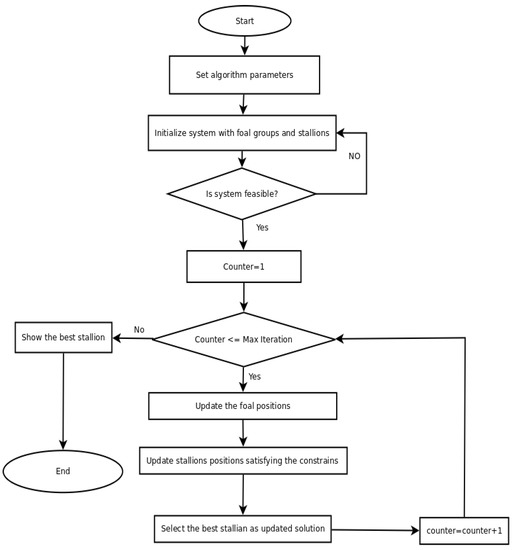
Figure 1.
Flow chart of MWHO.
2.1. Initialization, Group Construction and Stallion Selection
Initially, the population of horses is divided into several groups. Let denote the set of horses in the population. is the number of subsets with each subset representing a group. The algorithm assigns a leader, i.e., a stallion, to every group. Hence, there are stallions in the algorithm. The remaining population consists of foals and mares are further distributed among these groups. Each stallion, foal and mare represent a matrix of size , where is an upper bound in the number of the components in each of the q subsystems. The elements of the matrix represent the reliability of the components in each of the subsystems.
2.2. Grazing Behaviour of a Wild Horse
The majority of time is spent by foals and mares grazing in their group with a stallion at the centre of the grazing region [42]. Equation (1) simulates this grazing behaviour of wild horses.
where denotes the current position of the subset member in the pth subset. is the state variable associated with the stallion in subset q. is computed using Equation (2), which represents the adaptive nature of wild horses. represents a random number following uniform distribution in the range [−2, 2]. Finally, gives the updated values of the state variables associated with the subset member during grazing. The term in Equation (1) is a scaling of the vector, which determines the direction distance between the stallion and the member. Adding to this term i.e., the right side of the equation, represents the repositioning of the member along the vector joining the position of the stallion and the member. In other words, Equation (1) provides the new position of the member depending on the sign of the cosine term away from or towards the stallion, and thus the equation also determines the force between the stallion and the member. If the force is positive, the stallion pulls the member towards itself; if not, it repels the member away. The variables in Equation (1) are matrices of size and the reliability of each of the components in the subsystem are updated according to Equation (1).
Here, denotes a matrix with elements either 0 or 1. The elements in the matrices and follow uniform distribution in the range . is, again, a random number following uniform distribution in the range . The indices of the random matrix masked with following the positions where Q is zero in Equation (2) (The operator == in the equation is a logical operator aligned with the == operator in MATLAB or Python programming language). The operator ~; represents the negation i.e., if x = 0 (FALSE) then ~x will return 1 (TRUE). The operator represents elementwise multiplication; in the expression , both and are numbers; therefore, the elementwise multiplication reduces to normal multiplication between two numbers. In the expression , the operands of the operator + are a number on the left and a matrix on the right. The number on the left operand transforms itself into a matrix of the same size as the right operand, and all the elements of the matrix as the left operand. represents a dynamic parameter lying between [0, 1], which updates itself in accordance with Equation (3) during the execution process of the algorithm.
where denotes an iteration counter with as the upper bound on the number of iterations. As discussed earlier, in the expression , the right operand (TDR) transforms itself into a matrix of the same size as and the operator acts as elementwise comparison operator. The position of the member is updated by using Equation (1), which is modulated by Equation (2) in conjunction with Equation (3). The value of TDR reduces as the iteration progresses, which leads to a reduction in the number of 1s in Q (Equation (2)), which further leads to a increase in the number of 1s in IDX. The increase in 1s in IDX bounds the variations among elements of Z, leading all the members to move at the same scale towards iterations. Therefore, the optimization algorithm does not behave abnormally and does not deviate from convergence in the last few iterations.
2.3. Breeding Behaviour of a Horse
Wild horses have developed a mechanism so that fathers cannot mate with their daughters or siblings, as the foals split from the group before reaching puberty. Equation (4) represents this behavior depending upon a operator [42].
where denotes the state space of the ith horse in the group who splits from the subset and leaves its place for a horse with parents who parted from groups and in addition to having reached puberty. is the state space of the jth foal from the subset , which leaves the group after reaching the puberty, mates with the horse with the state space , which then splits from group q. In Equation (4), the state of the vacated ith horse in the group is updated with the mean value of the position of the jth foal from the subset and horse from subset q. In addition, Equation (4) also suggest that the crossover takes place between elements from two distinct groups.
2.4. Leadership Behaviour
The leadership and competitive behaviour of stallions when moving towards water sources is represented by Equation (5) [42].
where , and denote the next position in state space of the leader in the pth group, the state of the water hole and the current state of the leading element of the pth subset, respectively. Equation (5a,b) behave in a similar way to Equation (2); however, here, the role of the stallion is taken by the global optimal and the role of the members is swapped for the stallions. Therefore, the global optimal position searched by the algorithm does not change abruptly from the convergence.
2.5. Leader Selection and Exchange
Finally, the leader is chosen based on their fitness or cost (Equation (6)) [42]. The leader’s position, along with the relevant member, will be modified by using Equation (6).
The original WHO algorithm [42] can be applied across a wide range of optimization problems. However, to apply the WHO for SROPs, certain modifications must be made. These include the change of one variable to matrix of size . We discuss here two classes of modifications, which are further required to use the proposed MWHO efficiently for SROPs. The first class of modification pertains to the application of constraints, which is not considered in the original WHO algorithm [42]. However, as the SROPs in question involve constraints (i.e., the constraints of overall system reliability () and components reliabilities ()), conditional steps are introduced to the WHO algorithm to accommodate these constraints. During the update process, these conditions are assessed against the constraints, and only if the constraints are met, the new positions of the horses are updated. The second class of modifications relates to the initialization process in MWHO algorithms.
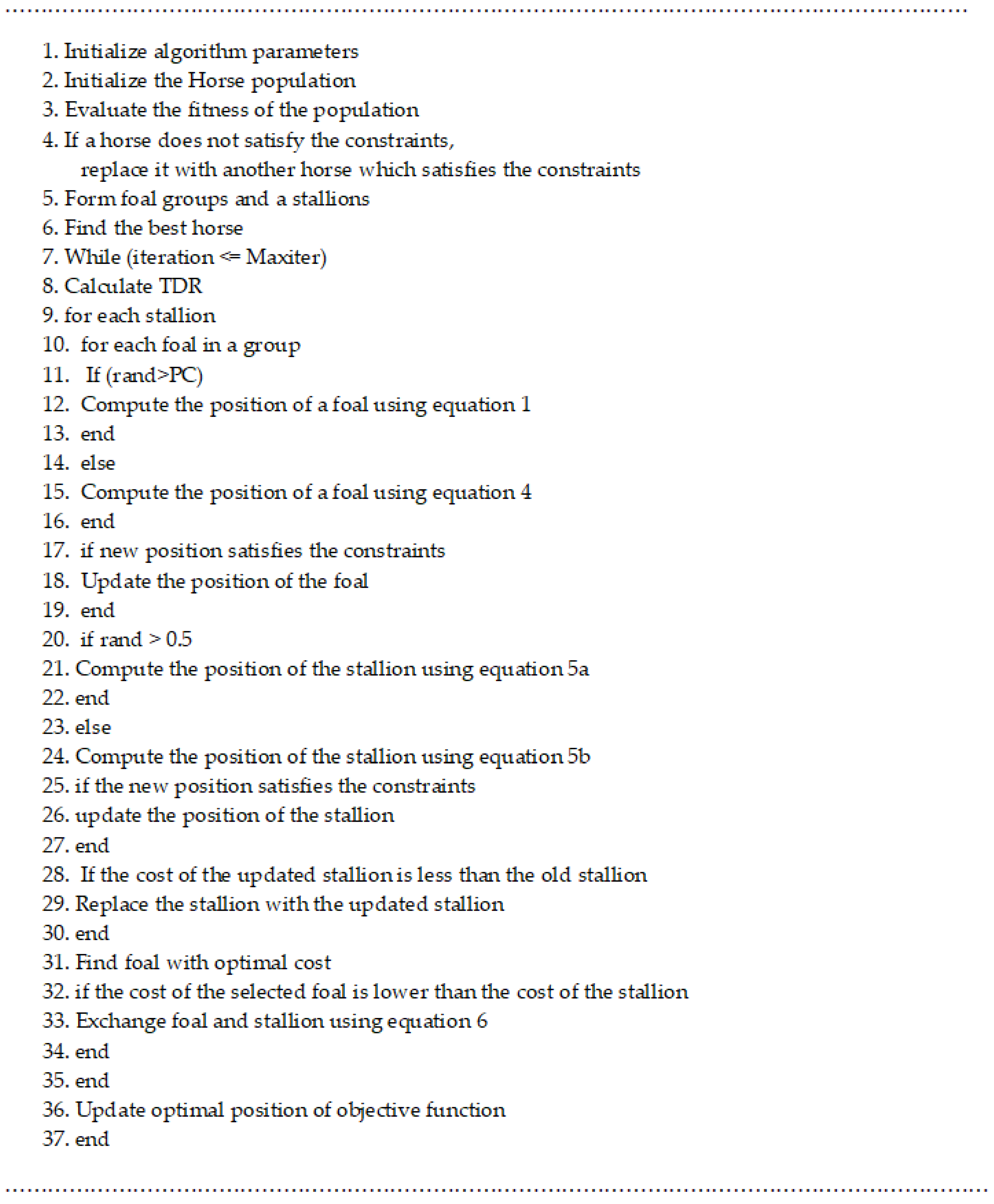
While the horse population is initialized with random values, these values may not adhere to the constraints, causing the horses to diverge or converge at a slow rate. To address this, each horse is compelled to start in the feasible region by iterating over multiple generations until a feasible solution is attained. This step is repeated for each member of the population. Figure 2 provides the pseudo-code for MWHO.
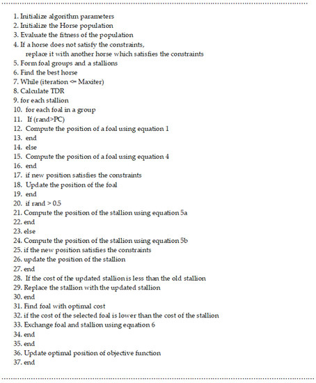
Figure 2.
Pseudo-code of the MWHO.
3. Problem Description
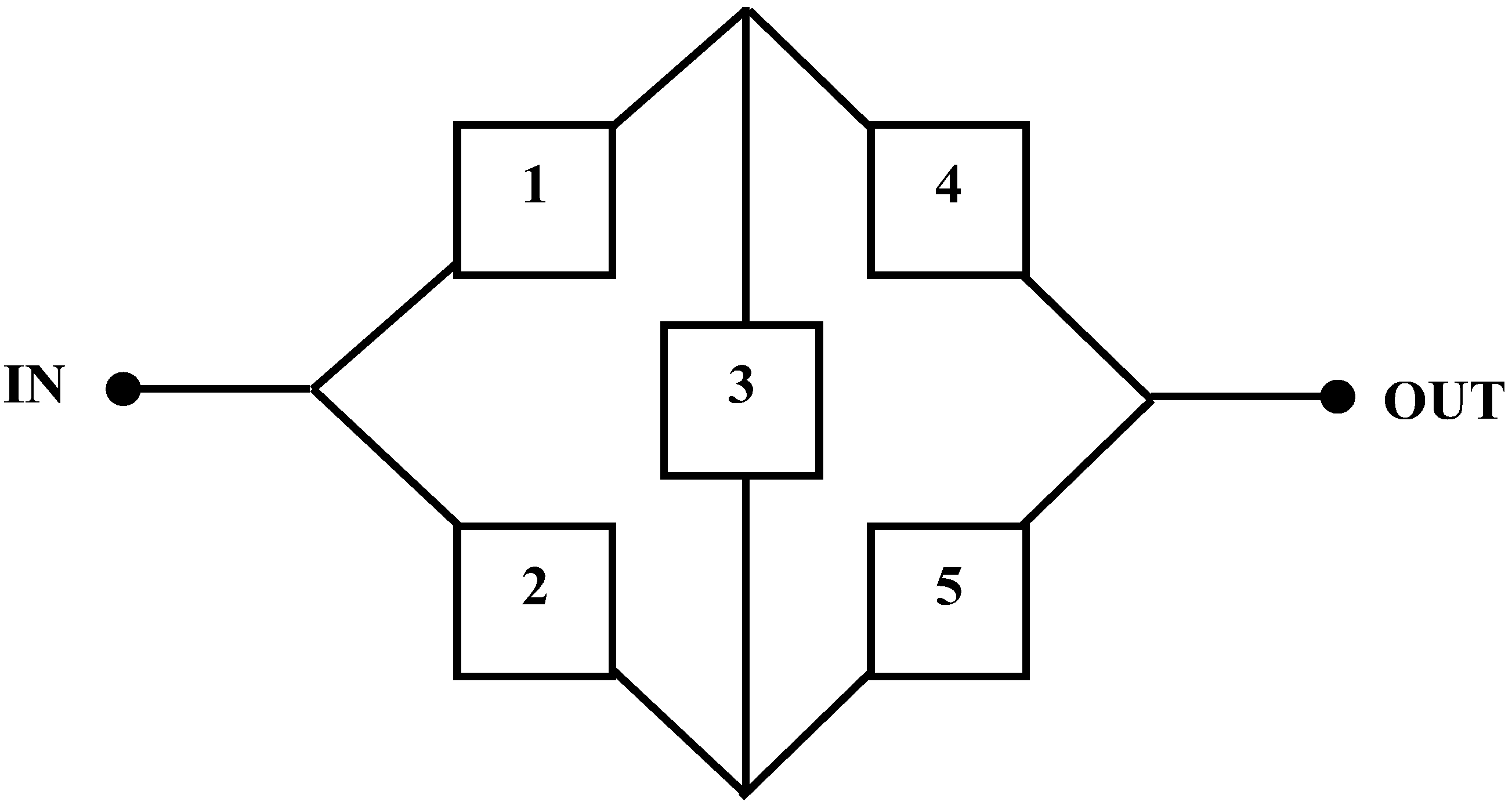
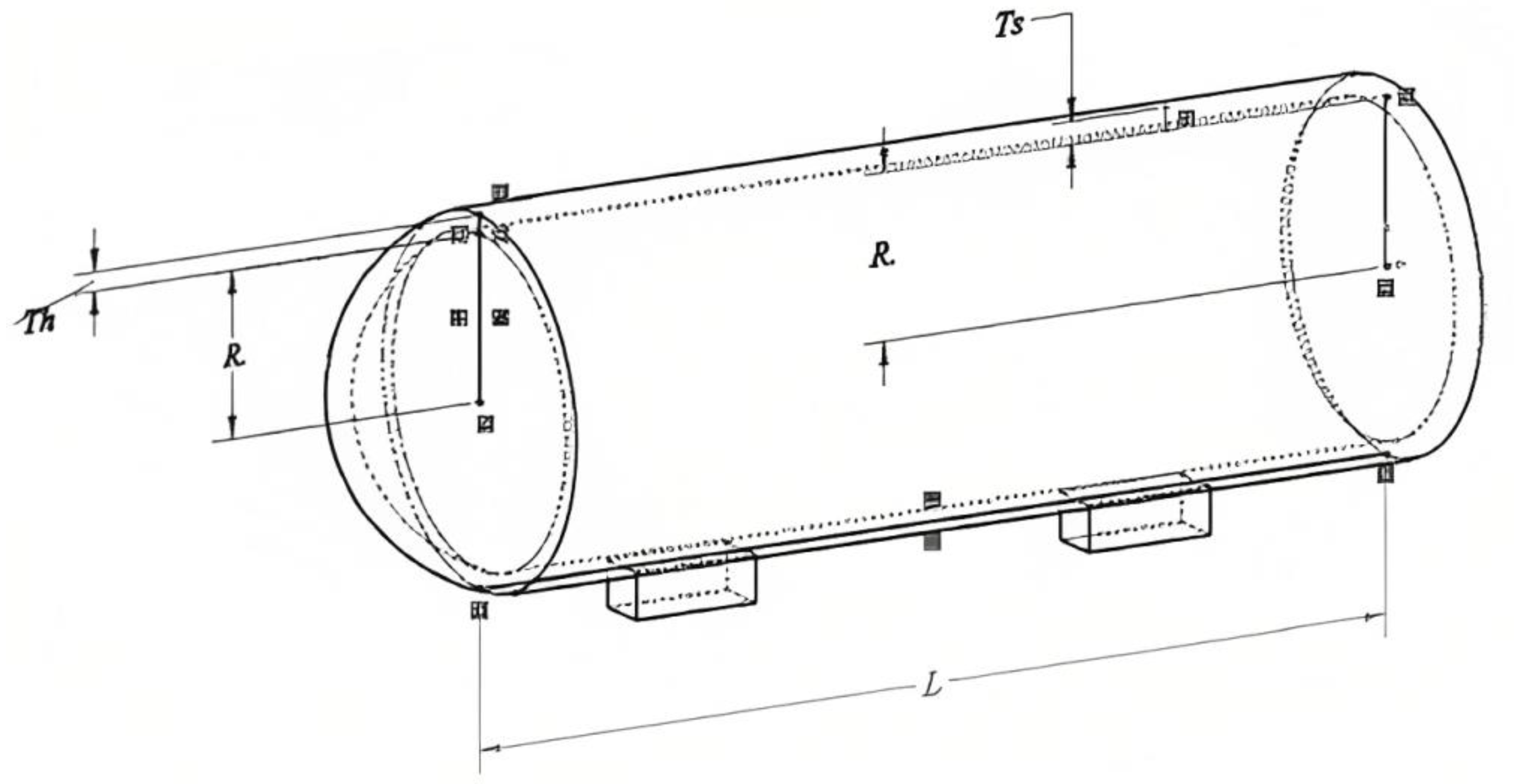
To check the applicability and efficiency of the MWHO, two SROPs and one engineering optimization problem (EOP) are considered here. The block diagram of the SROPs and EOP considered is depicted in Figure 3, Figure 4 and Figure 5.
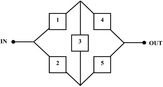
Figure 3.
Block diagram of SROP 1.
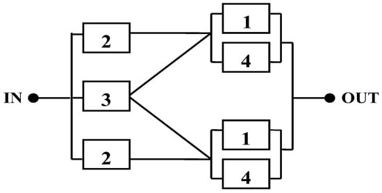
Figure 4.
Block diagram of SROP 2.
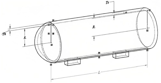
Figure 5.
Schematic of PVD.
3.1. Statement of the Optimization Problems
A general constraint optimization problem, which is non-linear in nature, can be defined as
A typical implementation consists of three fundamental elements: a collection of variables, a fitness function for optimization (either maximizing or minimizing), and a set of constraints that define the permissible range of values for the variables. The objective is to determine the optimal values for the variables that optimize the fitness (cost) function while adhering to the given constraints.
In SROP1 and SROP2, the objective is to minimize the associated system cost (),subject to the constraints of overall system reliability () and component reliabilities (). In EOP, the objective again is to minimize the total cost () consisting of material, forming and welding of a cylindrical vessel subjected to various constraints formed by the decision variables, namely, thickness of the shell (), thickness of the head (), inner radius (), length of the cylindrical section without considering the head ().
3.2. SROP 1: Complex Bridge System (CBS)
Solving a system that has a redundant unit and is not in a pure series configuration poses significant difficulty. The complex bridge system problem, depicted in Figure 3, is a prime example. This system consists of five components, each possessing a component reliability value of . The complex bridge system is composed of two subsystems: the first subsystem involves components 1 and 4 connected in series, while the second subsystem comprises components 2 and 5 in series. These two subsystems are connected in a parallel configuration, with component 3 inserted in between. Figure 3 depicts the block diagram of CBS.
The mathematical formulation of SROP 1, with the objective of minimizing overall system cost with nonlinear constraint, is given below [13]:
subjected to
3.3. SROP 2: Life Support System in Space Capsule (LSSSC)
The creation and analysis of physical habitat for space exploration is crucial to shield the astronaut from the harshness of space. Additionally, the LSSSC must be regenerative, providing essential elements for human survival. Figure 4 illustrates the block diagram of the LSSSC, which consists of four components, each with a reliability value of . The system requires a single path for successful operation and contains two redundant subsystems, with each subsystem comprising components 1 and 4. Both redundant subsystems are in a series with component 2, forming two identical paths in a series-parallel arrangement. Component 3 serves as a third path and backup for the pair. Component 1 is backed up by a parallel component 4, and two identical paths are created, each having component 2 in a series with the stage consisting of components 1 and 4. These two paths operate in parallel, so that if one of them functions correctly, the output is guaranteed.
where, I1 = 100, I2 = 100, I3 = 200, I4 = 150 and .
The mathematical formulation of SROP 2, with the objective of minimizing overall system cost with nonlinear constraint, is given below [13]:
subjected to
where Rk is the kth component’s reliability.
3.4. Engineering Optimization Problem (EOP): Pressure Vessel Design (PVD)
The objective of this EOP, named PVD, is to minimize the total cost () consisting of material, forming and welding of a cylindrical vessel, as presented in Figure 5. Both ends of the vessel are capped, and the head has a hemispherical shape. This EOP consists of four decision variables, namely, thickness of the shell (), thickness of the head (), inner radius () and length of the cylindrical section without considering the head () [38].
The mathematical formulation of this EOP is as follows:
subjected to
4. Results and Discussion
To evaluate the performance of the MWHO algorithm on SROPs, the proposed MWHO algorithm was implemented on the two SROPs describe in Section 3 using GNU Octave version 6.4.0 on a personal computer with the following performance: 11th Gen Intel Core I5-1135G7, 2.4 GHz * 8 and 16 GB of RAM. To obtain the best working combination of parameters for MWHO, a trial-and-error methodology was used.
The proposed algorithm was applied to these SROPs with the following parameters: For SROP 1: number of stallions, 40; crossover percentage, 20; number of iterations, 1000; and for SROP 2: number of stallions, 40; crossover percentage, 20; number of iterations, 500; and for EOP (PVD): number of stallions, 40; crossover percentage, 20; number of iterations, 100. The MWHO algorithm was executed independently for ten runs for each SROP and EOP (PVD). The best, worst, mean and standard deviation values for each run obtained by MWHO algorithm are reported in Table 2, Table 3 and Table 4.

Table 2.
Results of ten MWHO runs for SROP 1.

Table 3.
Results of ten MWHO runs for SROP 2.

Table 4.
Results of ten MWHO runs for the EOP (PVD).
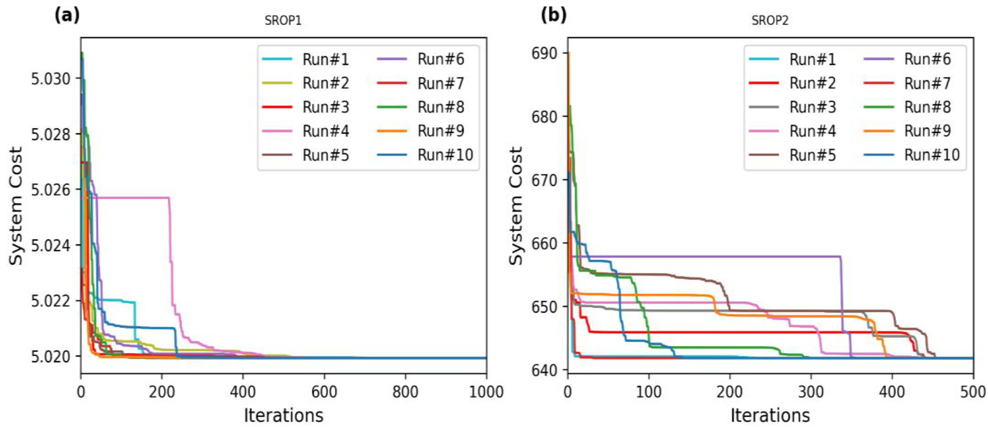
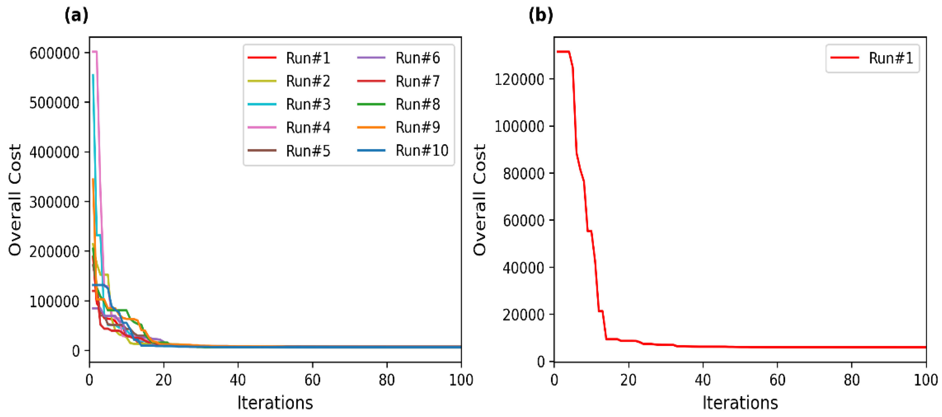
Figure 6 depicts the convergence curve obtained by MWHO in 10 different runs for SROP1 and SROP2.
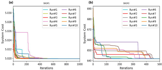
Figure 6.
Convergence curve obtained by MWHO in 10 different runs for SROPs (first 500 iterations). (a) SROP1 (b) SROP2.
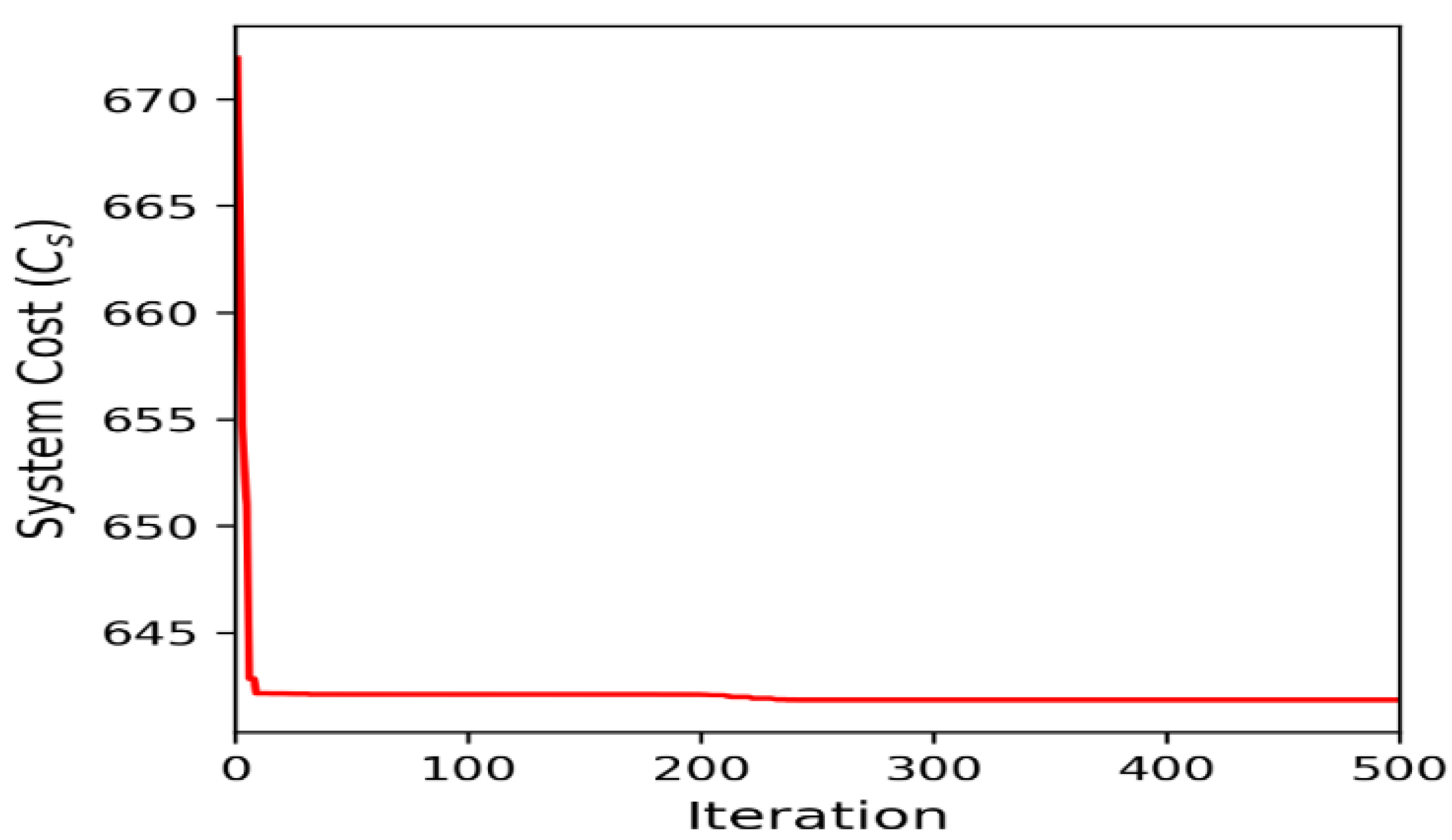
As shown in Figure 6, the system cost converges towards optimal value approximately after 600 iterations across the 10 runs in SROP1 (Figure 6a). On the other hand, the system cost converges towards optimal value approximately after 460 iterations in SROP2 (Figure 6b). Figure 7 and Figure 8 present the convergence curve of the best run for SROP 1 and SROP 2. For EOP (PVD), system cost converges towards optimal value after approximately 25 iterations (Figure 9a). It is also observed that the initial values taken by the optimization algorithm have little effect on the convergence towards the optimal points. However, some initial values can lead to reaching the optimal point faster than some other initial values of the parameters. As shown in Figure 7, Figure 8 and Figure 9b, the best run, defined as the run providing minimum cost, converges towards the optimal point faster than most of the runs. We do not conclude that faster convergence means the best solution, as in Figure 6a, run #9 shows a lower system cost compared to the best run (run #3). However, a faster convergence does have an advantage, as the search particles can descend towards the optimal point faster and save computational time.
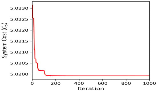
Figure 7.
Convergence curve of SROP 1.
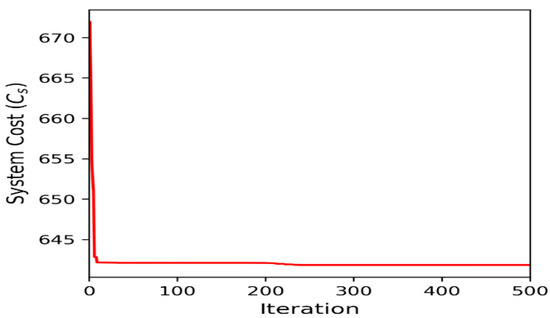
Figure 8.
Convergence curve of SROP 2.
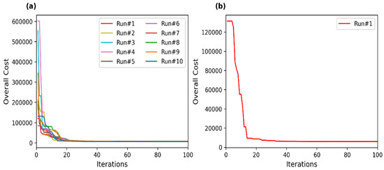
Figure 9.
(a) Convergence curve obtained by MWHO in 10 different runs for EOP (PVD) (b) Convergence curve of EOP (PVD).
Table 2, Table 3 and Table 4 provide the statistical results of MWHO for SROP1, SROP2 and EOP (PVD), respectively. They reflect the minimum (best), maximum (worst), mean and standard deviation of the system cost for each run in fixed iterations. Based on the convergence curves (Figure 6, Figure 7, Figure 8 and Figure 9) and statistical results presented in Table 2, Table 3 and Table 4, Run 3 has been identified as the best run for SROP1, Run 2 has been identified as the best run for SROP2, while Run 1 has been identified as the best run for EOP (PVD). Run 3 for SROP1 has a minimum system cost of 5.0199184060, with a mean cost of 5.0200024039 and a standard deviation of 0.0003699874, whereas Run 2 for SROP2 has a minimum system cost of 641.8235623261, with a mean cost of 642.1114292308 and a standard deviation of 1.8683118611. Run 1 for EOP (PVD) has a minimum system cost of 5885.332774, with a mean cost of 6005.540996 and a standard deviation of 2557.519377.
Comparison of the best results obtained by MWHO for SROP 1, SROP 2 and EOP (PVD) with other metaheuristics is presented in Table 5, Table 6 and Table 7, respectively.

Table 5.
Comparison of the best results for SROP 1 obtained using different algorithms.

Table 6.
Comparison of the best results for SROP 2 obtained using different algorithms.

Table 7.
Comparison of the best results for the EOP (PVD) obtained using different algorithms.
The results for SROP1 obtained by the MWHO algorithm, along with a few other results, are presented in Table 5. The table demonstrates that the MWHO yields significant improvements over solutions obtained using PSO, GWO, CSA and ACO. With only 40,000 function evaluations, MWHO achieved a minimum system cost of 5.0199184060 while maintaining system reliability of 0.9900000000.
The results for SROP2 obtained by the MWHO algorithm, along with a few other results, are presented in Table 6. The table demonstrates that MWHO provides very competitive results when compared to solutions obtained using PSO, GWO, CSA and ACO. With 20,000 function evaluations, MWHO achieved a minimum system cost of 641.8235623261 while maintaining system reliability of 0.9000000000.
The results for EOP (PVD) obtained by the MWHO algorithm, along with a few other results, are presented in Table 7. The table demonstrates that MWHO yields significant improvements when compared to solutions obtained using PSO, GWO, GA and ACO. With only 4000 function evaluations, MWHO achieved a minimum system cost of 5885.332774.
5. Conclusions and Future Scope
The objective of this article was to introduce a solution approach based on MWHO to deal with SROPs. The proposed MWHO, which is a modified version of WHO, has high performance on SROPs and can handle them with great ease. In addition, the comparative analysis with the results available in the literature dealing with the same SROPs shows that the MWHO algorithm has better efficiency, as it provides either superior or comparable solutions. For further study, our work will be devoted to the development of a hybrid multi-objective version of the MWHO algorithm to deal with multi-objective SROPs. Additionally, analysing the applicability, efficiency and stability of the MWHO on real life engineering cases such as Failure Mode Effects Analysis [43], Bayesian Network predictive analysis, and combining MWHO with some MCDM techniques may be expwereed [44,45].
Author Contributions
A.K. (Anuj Kumar): Conceptualization, Investigation, Methodology, Draft preparation. S.P.: Conceptualization, Investigation and drafting. M.K.S.: Programming, Investigation. S.C.: Conceptualization, Investigation and drafting. M.R.: Drafting, Investigation. A.K. (Akshay Kumar): Drafting, Investigation. All authors have read and agreed to the published version of the manuscript.
Funding
This research received no external funding.
Data Availability Statement
Not applicable.
Conflicts of Interest
The authors declare no conflict of interest.
References
- Charles, E.E. An Introduction to Reliability and Maintainability Engineering; McGraw Hill: New York, NY, USA, 1997. [Google Scholar]
- Kumar, A.; Ram, M.; Pant, S.; Kumar, A. Industrial system performance under multistate failures with standby mode. In Modeling and Simulation in Industrial Engineering; Springer: Cham, Switzerland, 2018; pp. 85–100. [Google Scholar]
- Yazdi, M.; Mohammadpour, J.; Li, H.; Huang, H.Z.; Zarei, E.; Pirbalouti, R.G.; Adumene, S. Fault tree analysis improvements: A bibliometric analysis and literature review. Qual. Reliab. Eng. Int. 2023, Early View. [Google Scholar] [CrossRef]
- Li, H.; Yazdi, M.; Huang, H.Z.; Huang, C.G.; Peng, W.; Nedjati, A.; Adesina, K.A. A fuzzy rough copula Bayesian network model for solving complex hospital service quality assessment. Complex Intell. Syst. 2023, 1–27. [Google Scholar] [CrossRef]
- Pant, S.; Kumar, A.; Ram, M. Reliability optimization: A particle swarm approach. In Advances in Reliability and System Engineering; Springer: Cham, Switzerland, 2017; pp. 163–187. [Google Scholar]
- Kumar, A.; Pant, S.; Ram, M.; Yadav, O. (Eds.) Meta-Heuristic Optimization Techniques: Applications in Engineering; Walter de Gruyter GmbH & Co KG: Berlin, Germany, 2022; Volume 10. [Google Scholar]
- Coit, D.W.; Smith, A.E. Reliability optimization of series-parallel systems using a genetic algorithm. IEEE Trans. Reliab. 1996, 45, 254–260. [Google Scholar] [CrossRef]
- Liang, Y.-C.; Smith, A.E. An ant colony optimization algorithm for the redundancy allocation problem (RAP). IEEE Trans. Reliab. 2004, 53, 417–423. [Google Scholar] [CrossRef]
- Wolpert, D.H.; Macready, W.G. No free lunch theorems for optimization. IEEE Trans. Evol. Comput. 1997, 1, 67–82. [Google Scholar] [CrossRef]
- Modibbo, U.M.; Arshad, M.; Abdalghani, O.; Ali, I. Optimization and estimation in system reliability allocation problem. Reliab. Eng. Syst. Saf. 2021, 212, 107620. [Google Scholar] [CrossRef]
- Ouzineb, M.; Nourelfath, M.; Gendreau, M. Tabu search for the redundancy allocation problem of homogenous series–parallel multi-state systems. Reliab. Eng. Syst. Saf. 2008, 93, 1257–1272. [Google Scholar] [CrossRef]
- Beji, N.; Jarboui, B.; Eddaly, M.; Chabchoub, H. A hybrid particle swarm optimization algorithm for the redundancy allocation problem. J. Comput. Sci. 2010, 1, 159–167. [Google Scholar] [CrossRef]
- Kumar, A.; Pant, S.; Ram, M. System reliability optimization using gray wolf optimizer algorithm. Qual. Reliab. Eng. Int. 2017, 33, 1327–1335. [Google Scholar] [CrossRef]
- Hsieh, Y.-C.; You, P.-S. An effective immune based two-phase approach for the optimal reliability–redundancy allocation problem. Appl. Math. Comput. 2011, 218, 1297–1307. [Google Scholar] [CrossRef]
- Wu, P.; Gao, L.; Zou, D.; Li, S. An improved particle swarm optimization algorithm for reliability problems. ISA Trans. 2011, 50, 71–81. [Google Scholar] [CrossRef]
- Zou, D.; Gao, L.; Li, S.; Wu, J. An effective global harmony search algorithm for reliability problems. Expert Syst. Appl. 2011, 38, 4642–4648. [Google Scholar] [CrossRef]
- Hsieh, T.-J.; Yeh, W.-C. Penalty guided bees search for redundancy allocation problems with a mix of components in series–parallel systems. Comput. Oper. Res. 2012, 39, 2688–2704. [Google Scholar] [CrossRef]
- Lins, I.D.; Droguett, E.L. Redundancy allocation problems considering systems with imperfect repairs using multi-objective genetic algorithms and discrete event simulation. Simul. Model. Pract. Theory 2011, 19, 362–381. [Google Scholar] [CrossRef]
- Wang, L.; Li, L.-P. A coevolutionary differential evolution with harmony search for reliability–redundancy optimization. Expert Syst. Appl. 2012, 39, 5271–5278. [Google Scholar] [CrossRef]
- Wang, Y.; Li, L. Heterogeneous redundancy allocation for series-parallel multi-state systems using hybrid particle swarm optimization and local search. IEEE Trans. Syst. Man Cybern. Part A Syst. Hum. 2012, 42, 464–474. [Google Scholar] [CrossRef]
- Pourdarvish, A.; Ramezani, Z. Cold standby redundancy allocation in a multi-level series system by memetic algorithm. Int. J. Reliab. Qual. Saf. Eng. 2013, 20, 1340007. [Google Scholar] [CrossRef]
- Valian, E.; Valian, E. A cuckoo search algorithm by Lévy flights for solving reliability redundancy allocation problems. Eng. Optim. 2013, 45, 1273–1286. [Google Scholar] [CrossRef]
- Valian, E.; Tavakoli, S.; Mohanna, S.; Haghi, A. Improved cuckoo search for reliability optimization problems. Comput. Ind. Eng. 2013, 64, 459–468. [Google Scholar] [CrossRef]
- Afonso, L.D.; Mariani, V.C.; dos Santos Coelho, L. Modified imperialist competitive algorithm based on attraction and repulsion concepts for reliability-redundancy optimization. Expert Syst. Appl. 2013, 40, 3794–3802. [Google Scholar] [CrossRef]
- Ardakan, M.A.; Hamadani, A.Z. Reliability optimization of series–parallel systems with mixed redundancy strategy in subsystems. Reliab. Eng. Syst. Saf. 2014, 130, 132–139. [Google Scholar] [CrossRef]
- Yeh, W.-C. Orthogonal simplified swarm optimization for the series–parallel redundancy allocation problem with a mix of components. Knowl. Based Syst. 2014, 64, 1–12. [Google Scholar] [CrossRef]
- Kumar, A.; Negi, G.; Pant, S.; Ram, M.; Dimri, S.C. Availability-Cost Optimization of Butter Oil Processing System by Using Nature Inspired Optimization Algorithms. Reliab. Theory Appl. 2021, 64, 188–200. [Google Scholar]
- Huang, C.-L. A particle-based simplified swarm optimization algorithm for reliability redundancy allocation problems. Reliab. Eng. Syst. Saf. 2015, 142, 221–230. [Google Scholar] [CrossRef]
- He, Q.; Hu, X.; Ren, H.; Zhang, H. A novel artificial fish swarm algorithm for solving large-scale reliability–redundancy application problem. ISA Trans. 2015, 59, 105–113. [Google Scholar] [CrossRef]
- Ardakan, M.A.; Hamadani, A.Z.; Alinaghian, M. Optimizing bi-objective redundancy allocation problem with a mixed redundancy strategy. ISA Trans. 2015, 55, 116–128. [Google Scholar] [CrossRef]
- Zhuang, J.; Li, X. Allocating redundancies to k-out-of-n systems with independent and heterogeneous components. Commun. Stat.-Theory Methods 2015, 44, 5109–5119. [Google Scholar] [CrossRef]
- Garg, H. An approach for solving constrained reliability-redundancy allocation problems using cuckoo search algorithm. Beni-Suef Univ. J. Basic Appl. Sci. 2015, 4, 14–25. [Google Scholar] [CrossRef]
- Mellal, M.A.; Zio, E. A penalty guided stochastic fractal search approach for system reliability optimization. Reliab. Eng. Syst. Saf. 2016, 152, 213–227. [Google Scholar] [CrossRef]
- Abouei Ardakan, M.; Sima, M.; Zeinal Hamadani, A.; Coit, D.W. A novel strategy for redundant components in reliability-redundancy allocation problems. IIE Trans. 2016, 48, 1043–1057. [Google Scholar] [CrossRef]
- Gholinezhad, H.; Hamadani, A.Z. A new model for the redundancy allocation problem with component mixing and mixed redundancy strategy. Reliab. Eng. Syst. Saf. 2017, 164, 66–73. [Google Scholar] [CrossRef]
- Kim, H.; Kim, P. Reliability models for a nonrepairable system with heterogeneous components having a phase-type time-to-failure distribution. Reliab. Eng. Syst. Saf. 2017, 159, 37–46. [Google Scholar] [CrossRef]
- Kim, H. Maximization of system reliability with the consideration of component sequencing. Reliab. Eng. Syst. Saf. 2018, 170, 64–72. [Google Scholar] [CrossRef]
- Garg, H. A hybrid GSA-GA algorithm for constrained optimization problems. Inf. Sci. 2019, 478, 499–523. [Google Scholar] [CrossRef]
- Al-Azzoni, I.; Iqbal, S. Meta-heuristics for solving the software component allocation problem. IEEE Access 2020, 8, 153067–153076. [Google Scholar] [CrossRef]
- Kumar, A.; Pant, S.; Ram, M. Gray wolf optimizer approach to the reliability-cost optimization of residual heat removal system of a nuclear power plant safety system. Qual. Reliab. Eng. Int. 2019, 35, 2228–2239. [Google Scholar] [CrossRef]
- Negi, G.; Kumar, A.; Pant, S.; Ram, M. Optimization of complex system reliability using hybrid grey wolf optimizer. Decis. Mak. Appl. Manag. Eng. 2021, 4, 241–256. [Google Scholar] [CrossRef]
- Naruei, I.; Keynia, F. Wild horse optimizer: A new meta-heuristic algorithm for solving engineering optimization problems. Eng. Comput. 2021, 38, 3025–3056. [Google Scholar] [CrossRef]
- Li, H.; Soares, C.G.; Huang, H.Z. Reliability analysis of a floating offshore wind turbine using Bayesian Networks. Ocean Eng. 2020, 217, 107827. [Google Scholar] [CrossRef]
- Pant, S.; Garg, P.; Kumar, A.; Ram, M.; Kumar, A.; Sharma, H.K.; Klochkov, Y. AHP-based multi-criteria decision-making approach for monitoring health management practices in smart healthcare system. Int. J. Syst. Assur. Eng. Manag. 2023, 1–12. [Google Scholar] [CrossRef]
- Li, H.; Díaz, H.; Soares, C.G. A failure analysis of floating offshore wind turbines using AHP-FMEA methodology. Ocean. Eng. 2021, 234, 109261. [Google Scholar] [CrossRef]
Disclaimer/Publisher’s Note: The statements, opinions and data contained in all publications are solely those of the individual author(s) and contributor(s) and not of MDPI and/or the editor(s). MDPI and/or the editor(s) disclaim responsibility for any injury to people or property resulting from any ideas, methods, instructions or products referred to in the content. |
© 2023 by the authors. Licensee MDPI, Basel, Switzerland. This article is an open access article distributed under the terms and conditions of the Creative Commons Attribution (CC BY) license (https://creativecommons.org/licenses/by/4.0/).


