Abstract
This paper presents a set of adaptive parameter control methods through reinforcement learning for the particle swarm algorithm. The aim is to adjust the algorithm’s parameters during the run, to provide the metaheuristics with the ability to learn and adapt dynamically to the problem and its context. The proposal integrates Q–Learning into the optimization algorithm for parameter control. The applied strategies include a shared Q–table, separate tables per parameter, and flexible state representation. The study was evaluated through various instances of the multidimensional knapsack problem belonging to the -hard class. It can be formulated as a mathematical combinatorial problem involving a set of items with multiple attributes or dimensions, aiming to maximize the total value or utility while respecting constraints on the total capacity or available resources. Experimental and statistical tests were carried out to compare the results obtained by each of these hybridizations, concluding that they can significantly improve the quality of the solutions found compared to the native version of the algorithm.
Keywords:
reinforcement learning; learning–based hybridizations; particle swarm optimization; mathematical combinatorial problem MSC:
65K05; 68T05; 68T20; 68W25; 68W50; 78M50; 90C59
1. Introduction
Nature–inspired optimization techniques are a set of algorithms or methods designed to adapt and solve complex optimization problems [1]. The level of adaptability of metaheuristics is because they do not depend on the mathematical structure of the problem but are based on heuristic procedures and intelligent search strategies [2,3]. There is a subset of metaheuristics known as swarm intelligence methods which are defined as procedures that operate based on a population of artificial individuals who can cooperate with each other to try to find the solution to the problem. Solutions can be classified as good enough and are found in a certain time, configured through the input parameters, which dictate the internal behavior of the execution [4].
Particle swarm optimization (PSO) is probably the bio-inspired optimization algorithm most applied in the last decades [5]. This method uses inertia weights, acceleration coefficients, and social coefficients to calculate the movement of its individuals in the search space. The parameters are so relevant in the execution and performance of the algorithm that, by making small adjustments, you can directly impact the result found [6]. Based on the “No Free Lunch” theorem, we can infer that no universal configuration for this algorithm can provide us with the best possible solution for all optimization problems [7]. Therefore, adapting the algorithm to the problem in question is necessary, considering the parameters that must be readjusted when facing different problems. It has been shown that parameter setting drastically affects the final result of the algorithm, and it is still a hot topic [8]. From this, the problem of parameter adjustment arises, which can be considered an optimization problem [9]. There are at least two ways to approach the problem of parameter tuning: (a) offline tuning, which implies the identification of the best values for a problem during a testing phase, and which does not modify the parameters during the execution of the algorithm, and (b) online control, which adapts the values of the parameters during execution, according to different strategies that can be deterministic, adaptive or self–adaptive. Due to the lack of a single solution to this problem, the scientific community has searched for hybrid modules inspired by different disciplines to provide a solution. One of these methods is Learnheuristics, which combines machine learning (ML) techniques with metaheuristic algorithms [10].
This study aims to investigate and develop different online parameter control strategies for swarm intelligence algorithms at runtime through reinforcement learning [11]. The proposal contemplates integrating a variety of Q–Learning algorithms into the PSO algorithm to assist in the control of its parameters online. Each variety of Q–Learning has its unique characteristics and adapts to different situations, making it possible to effectively address a variety of scenarios. The first strategy includes Q–Learning where the Q–table stores new parameter values of PSO. The second one integrates one table for each parameter, and finally, the third method is free for states. In order to demonstrate that the different technical proposals are viable, and to compare the performance of each one, some of the most challenging instances of the multidimensional knapsack Problem (MKP) will be solved. MKP is a wide-known NP-complete optimization problem consisting of items with profit and n–dimensional weight, and knapsacks that have been filled [12]. The objective is to choose a subset of items with maximum profits without exceeding the knapsack capacities. This problem was selected because it has a wide range of practical applications and continues to be a topic of interest in the operations research community [13,14,15]. For computational experiments, 70 of the most challenging instances of the MKP taken from the OR–Library [16] were used. The results were evaluated through descriptive analysis and statistical inferences, mainly a hypothesis contrast applying non–parametric evaluations.
The rest of the manuscript is divided as follows: Section 2 presents a robust analysis of the current relationship work on hybridizations between learning techniques and metaheuristics. Section 3 details the conceptual framework of the study. Section 4 explains how reinforcement learning techniques are applied on particle swarm optimization. Section 5 exposes the phases of the experimental design, while Section 6 discusses the results achieved. Finally, the conclusions and future work are given in Section 7.
2. Related Work
In recent years, the integration between swarm intelligence algorithms and machine learning has been extensively investigated [10]. To this end, various approaches have been described to implement self-adaptive and learning capabilities in these techniques. For example, in ref. [17], the virus optimization algorithm is modified to add self-adaptive capacities in the parameters. The performance was compared with different-sized optimization instances, and similar or better performance was observed for the improved version. Similarly, in ref. [18], the firefly algorithm was enhanced to auto-compute the parameter a that controls the balance between exploration and exploitation. In ref. [19], an analogous strategy modifies the cuckoo search algorithm to balance the intensification and diversification phases. The work published in [20] proposes improving the artificial bee colony by incorporating self-adaptive capabilities of its agents. This study aims to improve the convergence ratio by altering the parameter that controlled it during the run. A comparable work can be seen in [21]. Here, the differential evolution strategy is modified by adding auto–tuning qualities to the scalability factor and the crossing ratio to increase the convergence rate. The manuscript [22] describes an improvement of the discrete particle swarm optimization algorithm, which includes an adaptive parameter control to balance social and cognitive learning. A new formulation updates the probability factor in the Bernoulli distribution, which updates the parameters (social learning) and (cognitive learning). Following the same line, in [23,24], self-adaptive evolutionary algorithms were proposed. The first one details an enhancement through a population of operators that change based on a punishment and reward scheme, depending on the operator’s quality. The second one presents an improvement where the crossover and mutation probability parameters are adapted to balance exploration and exploitation in the search for solutions. Both cases show outstanding results. In ref. [25], a self-adjust was applied to the flower pollination algorithm. This proposal balances the exploration and exploitation phases during the run and uses a parameter as an adaptive strategy. A recent wolf pack algorithm was altered to auto-tune its parameter w that controls prey odor perception [26]. Here, the new version intensifies the local search toward more promising zones. Finally, the work in [27] proposes integrating the autonomous search paradigm in the dolphin echolocation algorithm for population self-regulation. The paradigm is applied when stagnation of a local optimum is detected.
Integrating metaheuristics with machine learning, regression, and clustering techniques has also been the subject of studies [28,29,30,31,32]. For example, in ref. [33], the authors propose an evolutionary algorithm that controls the parameters and operators. This is accomplished by integrating a controller module that applies learning rules, measuring the impact and assigning restarts to the parameter set. Under this same paradigm, the work reported in [34] explores the integration of the variable neighborhood search algorithm with reinforcement learning, applying reactive techniques for parameter adjustment, and selecting local searches to balance the exploration and exploitation phases. In ref. [35], a machine learning model was developed using the support vector machine, which can predict the quality of solutions for a problem instance. This solution then adjusts the parameters and guides the metaheuristics to more promising search regions. In ref. [36,37], the authors propose the integration of PSO with regression models and clustering techniques for population management and parameter tuning, respectively. In ref. [38], another combination between PSO and classifier algorithms is presented with the goal of deparameterizing the optimization method. In this approach, a previously trained model is used to classify the solutions found by the particles, which improves the exploration of the search space and the quality of the solutions obtained. Similar to previous works, in ref. [39], PSO is again enhanced with a learning model to control its parameters, obtaining a competitive performance compared to other parameter adaptation strategies. The manuscript [40] presents the hybridization between PSO, Gaussian Process Regression, and Support Vector Machine for real–time parameter adjustment. The study concluded that the hybrid offers superior performance compared to traditional approaches. The work presented in ref. [41] integrates randomized priority search with the Inductive Decision Tree data mining algorithm for parameter adjustment through a feedback loop. Finally, in ref. [42], the authors propose the integration of algorithms derived from ant colony optimization with fuzzy logic for the control of the parameters of pheromone evaporation rate, exploration probability factor, and the number of ants for solving the feature selection problem.
More specifically, reviewing studies on integrating metaheuristics and reinforcement learning, we find many works combining these two techniques to improve the search in optimization problems [43]. For example, in [44], the authors proposed the integration of bee swarm optimization with Q–Learning to improve their local search. In this approach, the artificial individuals become intelligent agents that gain and accumulate knowledge as the algorithm progresses, thus improving the effectiveness of the search. Along the same lines, ref. [45] proposes integrating a learning–based approach to the ant colony algorithm to control its parameters. It is carried out by assigning rewards to the change of parameters in the algorithm, storing them in an array, and learning the best values to apply to each parameter at runtime. In [46], another combination of a metaheuristic algorithm with reinforcement learning techniques is proposed. In this case, tabu search was integrated with Q–Learning to find promising regions in the search space when the algorithm is stuck at a local optimum. The work published in [47] also explored the application of reinforcement learning techniques in the context of an optimization problem. Here, the biased–randomized heuristic with reinforced learning techniques was studied to consider the variations generated by the change in the rewards obtained. Finally, Ref. [48] presents the implementation of a Q–Learning algorithm to assist in training neural networks to classify medical data. In this approach, a parameter tuning process was carried out in radial–based neural networks using Stateless Q–Learning. Although the latter is not an optimization algorithm, the work is relevant to our research.
Even though machine learning techniques have already been explored in bio-inspired algorithms, it is worth continuing research on this type of hybridization. Our strategy involves reinforcement learning on PSO, using Q–Learning and new variations that have not been studied yet. In this context, we studied how Q–Learning can be modified to provide better results. This approach can be fruitful if done properly.
3. Preliminaries
3.1. Parameter Setting
Metaheuristic algorithms are characterized by a set of parameters governing their behavior. In the scientific literature, the adjustment of these parameters is an interesting issue and still an open challenge [8,9,49,50,51]. According to [8], parameter tuning can be formally defined as follows:
- Let A be an algorithm with , , …, parameters that affect its behavior.
- Let C be a configuration space (parameter setting), where each configuration describes the values of the parameters required by A.
- I defines a set of instances to be resolved by the algorithm A.
- m is a metric of A performance on an instance of set I given a configuration c.
Find the best configuration , resulting in optimal performance of A, when resolving an instance of the set I according to the metric m.
Parameter settings can be treated by applying at least two options: parameter tuning and parameter control. Parameter tuning is the process of finding those configurations that allow the algorithm to present the best possible performance when solving a specific type of problem. Different methods or algorithms can be used to find the desired configuration manually or automatically. These methods include F–Race, Sampling F–Race, Iterative F–Race, ParamILS, Sharpening, and Adaptive Capping. These methods perform parameter changes before the execution of the algorithm, thus being considered a lengthy offline process that requires a large number of executions for each configuration instance [52]. On the other hand, parameter control is considered an online process because it focuses on implementing parameter changes during the execution of the algorithm [53]. Parameter control is classified into three strategies: deterministic, adaptive, and self–adaptive [54]. The deterministic strategy uses deterministic rules to change the parameters and does not have a feedback system. The adaptive strategy uses feedback to vary the direction and magnitude of the parameter change. The self-adaptive strategy encodes the parameters of each individual in the population and modifies them in a certain number of iterations based on the best solutions found up to that moment.
3.2. Reinforcement Learning
Reinforcement learning is an algorithm part of ML whose objective is to determine the set of actions that an agent must take to maximize a given reward [11]. These agents need to be able to figure out for themselves which actions have the highest reward return, which is accomplished through trial and error. In some cases, these actions can yield long–term rewards, known as retroactive rewards. Trial and error and retroactive rewards are the two most important features of reinforcement learning [55,56].
Reinforcement learning employs a cycle involving several elements: the agent, the environment, the value function, the reward, the policy, and the model [57]. The agent is the element that performs actions in the environment by learning and incorporating new policies to follow in future actions. Policies vary based on the reward received for performing an action. The agent’s objective is to choose actions that increase the reward in the long term. The environment is where the agent’s actions are applied, and based on these actions, it is the place where the state changes will be caused. The value function uses these state changes to determine the impact of each action. The value function is the evaluator element within the algorithm. Its function is to evaluate each action carried out by the agent and its impact on the environment. This is achieved by assigning a reward to the action/state change pair and delivering it to the agent, thus completing the cyclic element. The reward is the numerical value that the value function assigns to an action/state change pair. Usually, a positive value indicates positive feedback, while a negative value indicates negative feedback. The policy is the element that gives the algorithm the ability to continuously learn, allowing the agent’s behavior to be defined during the execution of the algorithm. Generally, a policy maps the perceived states in the environment and the actions that must be taken in those states. Finally, the model is an optional element that serves as input into the agent’s decision making. Unlike policies, the model is static at runtime and only has predefined data.
Uncertainty in Q–Learning can affect the exploration phase of PSO. This can impact the convergence and quality of solutions generated by PSO. The relationship between the learning uncertainty Q–Learning and the PSO is complex and depends on several factors, such as the configuration of the algorithm and the interaction between the parameters. This conflict remains latent among the scientific community. Optimization algorithms governed by learning methods continue to be a hot topic [58].
3.2.1. Q–Learning
Q–Learning is a model-free reinforcement learning algorithm introduced by C. Watkins in 1989 [59]. This algorithm introduces the Q function, which works as a table that stores the maximum expected rewards for each action performed in a given state. This function is defined as [60,61]:
where A is the set of actions applicable to the environment, is the set of possible states of the environment in the next iteration, is the current state, R is the reward given for changing the state, is the learning rate, and is the discount factor. The procedure of Q–Learning can be seen in Algorithm 1.
| Algorithm 1: Q–Learning pseudocode |
 |
3.2.2. Single State Q–Learning
In cases where it is difficult (or outright impossible) to determine the states of the system, there is the possibility of reducing Q–Learning to a single static state. This method is called Single State Q–Learning (or Stateless Q–Learning) [62,63]. Given the simplification of the algorithm, the table Q is transformed to an array, and the Equation (1) is abbreviated to the Equation (2):
where A is the set of actions applicable to the environment, R is the reward given for performing an action, and is the learning rate.
4. Developed Solution
In this section, we detail different ways to apply Q–Learning on PSO and how this implementation allows us to improve its performance when solving NP–Complete combinatorial optimization problems.
4.1. Particle Swarm Optimization
Particle swarm optimization is a swarm intelligence algorithm inspired by group behavior that occurs in flocks of birds and schools of fish [64]. In this algorithm, each particle represents a possible solution to the problem and has a velocity vector and a position vector.
PSO consists of a cyclical process in which each particle sees its trajectory influenced based on two types of learning: social learning, acquired through knowledge of other particles in the swarm, and cognitive learning, acquired through the experiences of the particle [5,65]. In the traditional PSO, the velocity of the particle is represented as a vector , as long as their position is described as . Initially, each particle’s position vector and velocity vector are randomly created. Then, during the execution of the algorithm, the particles are moved using the Equations (3) and (4):
where w is the acceleration coefficient, and are social learning and cognitive learning, respectively, and finally, and are uniformly distributed random values in the range . The method needs a memory, called , representing the best position met for the i–th particle. The best particle is stored in , and it is found when the algorithm ends. Algorithm 2 summarizes the PSO search procedure.
| Algorithm 2: PSO pseudocode |
 |
As a solution to the parameter optimization problem, integrating the Q–Learning algorithm in a traditional PSO is proposed. The objective of this combination is focused on PSO that can acquire the ability to adapt its parameters online, that is, during the execution of the algorithm.
The approach initializes by declaring the swarm, its particles, the necessary velocity vectors, and the Q table. The normal course for a PSO algorithm is then continued. The Q–Learning module is invoked when the algorithm is stagnation. We detect stagnation by applying the approximate theory of nature-inspired optimization algorithms, derived from , with uniform value in . This module analyzes the environment for possible state changes and then updates the Q table with the appropriate reward. If this is the first call to this module, these steps should be ignored. Subsequently, a decision must be made between two possible actions to adjust the algorithm’s parameters. One comes from the policy derived from Q, while the other option is to change the parameters randomly. The difference between these two options is that the first one will provide a better return depending on the existing knowledge. In contrast, the second one will allow us to find previously unknown knowledge. Finally, the Q–Learning module transfers control to PSO to continue operating. Figure 1 depicts the flow of the proposal.
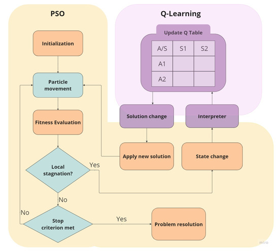
Figure 1.
Scheme of the proposal integrating a learning-based approach to the swarm intelligence method.
In the work, the proposed strategies allow us to integrate different levels of reinforced learning into swarm intelligence algorithms: Classic Q–Learning, Modified Q–Learning, and Single State Q–learning.
- (a)
- Classic Q–Learning (CQL): The first one directly applies the Q–Learning theory, including a single Q table. This table represents the states by combining the possible values of each parameter (in intervals of 0 and 1) and actions (transitions from one state to another). This process computes the fitness variation from the previous invoke to the module to the current call, assigning a positive or negative reward value according to the objective function. Then, the Q table is updated concerning the action/state pair. Finally, the most favorable action is derived according to the current state and the greedy policy, applying the new set of parameters to the swarm.
- (b)
- Modified Q–Learning (MQL): The second one is a variation of the classic Q–Learning. This strategy divides the Q table by each parameter and, furthermore, decreases the number of possible actions, allowing the agent only to move forward, backward, or stay in one state. In this method, the module is allowed to use each particle individually for the training of the Q tables and the modification of parameters. This means that, unlike the method seen above, this strategy is invoked only by one of the individuals in the swarm instead of the entire swarm. It is important to consider that each particle must store its current state and action as attributes such as velocity or position.
- (c)
- Single state Q–Learning (SSQL): The third one replaces the concept of a Q table with an array, removing states and looking only at changes produced by actions. The new Q array includes actions representing the parameter amount to modify. Similar to the previous version, the Q array has been split by each parameter and allows to use of the entire swarm individually. These changes effectively remove the state dependency, granting for more precise parameter changing.
4.2. Integration
Algorithm 3 shows the steps to follow to integrate reinforcement learning into PSO.
| Algorithm 3: Integration of reinforcement learning into PSO |
 |
Firstly, the procedure determines the states that represent the current condition or configuration of the PSO algorithm. These states could include the positions of the particles, their velocities, or any other relevant variables. Next, the algorithm identifies the actions that can be taken to modify the parameters of the PSO algorithm. These actions could involve changing the inertia weight, acceleration coefficients, or any other parameter that influences the behavior of the particles. In the third step, the method uses the reward function that evaluates the performance of the PSO algorithm based on the solutions obtained. The reward function should provide feedback on how well the algorithm is performing and guide the Q–learning process. The fourth step describes how the Q–table is created. Q–table is a lookup table that maps states and actions to their corresponding Q–values and it is initially filled with random elements.
The iterative process runs while PSO needs it. Here, the current state of PSO saves information, such as the positions and velocities of the particles, and the best solution found so far. Next, the most appropriate action is chosen based on the –greedy method. This method is employable because all actions are equally applicable. We consider the –greedy method as the policy to identify the best action. A uniform probability of where is used. The action modifies the parameter configuration of PSO in a random way: , where and . Then, PSO is executed to obtain the solutions. Its performance is evaluated by using the reward function and it allows to modify the Q–value of the previous state–action pair applying the Q–learning update rule. Finally, the previous state is updated to the current state, preparing for the next iteration of the algorithm. Over time, the Q-table will be updated, and the PSO algorithm will learn to select actions that lead to better solutions.
Before implementing, we analyze the time complexity of each component and its integration. Firstly, the time complexity of PSO depends mainly on the number of particles and the number of iterations. At each iteration, the positions and velocities of the particles are updated, and the objective function is evaluated. However, in this case, these components are constant, and the algorithm really depends on the dimensionality of the problem. Therefore, the complexity of the PSO algorithm itself is , where K represents the number of particles per number of iterations, and n defines the number of decision variables. On the other hand, the time complexity of Q–Learning is based on the size of the Q–table, which is determined by the number of possible states and actions. If the search space is large and the Q–table is large, the complexity will increase. In our case, we use a value range for parameters that remain constant during the run of PSO. Then, we can guarantee that the three proposals are efficient because none of them exceeds the polynomial time.
5. Experimental Setup
In order to comprehensively evaluate the performance of the proposed hybridizations, it is crucial to conduct a robust analysis that encompasses various aspects. One essential step in this analysis is to compare the solutions obtained by each strategy with the classic version of PSO. By benchmarking the solutions against the PSO’s results, we establish a reliable reference point for evaluating the effectiveness and efficiency of the proposed hybridizations. This enables us to gauge the extent to which the algorithmic enhancements contribute to improving solution quality and reaching optimality. Moreover, this comparative analysis serves to validate the credibility and competitiveness of the proposed hybridizations in the field. By showcasing their ability to achieve results that are on par with or even surpass PSO, we can establish the superiority of our approach and its potential to outperform existing methods.
To ensure the robustness of the performance analysis, it is important to employ a diverse set of benchmark problems that accurately represent the challenges and complexities encountered in real-world scenarios. By testing the proposed hybridizations on these benchmarks, we can assess their adaptability, generalizability, and ability to handle various problem instances effectively.
Figure 2 indicates the steps taken to examine the three proposals’ performance thoroughly. In addition, we establish objectives and recommendations for the experimental phase, in order to demonstrate that the proposed approaches allow for improving the optimization of metaheuristic parameters.
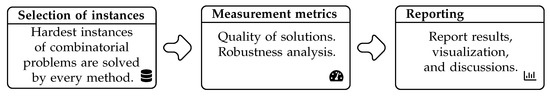
Figure 2.
Schema of the experimental phase applied to this work.
The analyses include: (a) the resolution time to determine the difference produced when applying the different methods, (b) the best value found by each method, which is an important indicator to assess future results, and finally, (c) an ordinal analysis and statistical tests to determine if one method is significantly better than another.
For the experimental phase, several optimization instances were solved in order to measure the performance of the different proposed methods. These instances were taken from the OR–Library, a virtual library that J.E. Beasley first described in 1990 [16], and in which it is possible to find various test data sets. In this study, 70 binary instances of the multidimensional knapsack problem were used (from MKP1 to MKP70). Table 1 details each instance, indicating its optimal solution, the number of backpacks, and the number of objects.

Table 1.
Instances of the multidimensional knapsack problem.
For instances from MKP56 to MKP70, there are no recorded optimal values because they could not be resolved by using exact methods. For this reason, we use “unknown” to describe that this value has not been found to date.
Equation (5) defines the formulation of MKP:
where describes whether or not the object is included in a backpack, and n represents the total number of objects. Each object has a real value that represents its profit and is used to calculate the objective function. Finally, stores the weight of each object based on the backpack k with maximum capacity . As can be seen, this is a combinatorial problem that deals with the dilemma of including or not an object in a certain backpack that has a certain capacity.
To execute a metaheuristic of a continuous nature in a binary domain, it is required to add a binarization phase after the solution vector changes [69]. Here, a standard sigmoid function was used as the transformation function, that is, , with as a uniform random value between . Then, if the previous formulation is true, we use as discretization. Otherwise, we use .
The performance of each method is evaluated after resolving each of the 70 instances a total of 30 times. Once the complete set of results is obtained from all executions and instances, an outlier analysis is performed to study possible irregular results. Here, influential outliers were detected using the Tukey test, which takes as reference the difference between the first quartile (Q1) and the third quartile (Q3), or the interquartile range. In our case, it is considered a slight outlier if the result is 1.5 times that distance from one of those quartiles or an extreme outlier if it is three times that distance. This test was implemented using a spreadsheet to calculate the statistical values automatically. All outliers were removed to avoid distortion of the samples, and then new tests were taken to replace the removed solutions. Moreover, we use the metric of the relative percentage difference (RPD) between the best solution to the problem and the best solution found. This value is calculated on .
As a next step, a descriptive and statistical analysis of the results was carried out. For the first, metrics such as maximum and minimum values, the mean, the quasi–standard deviation, the median, and the interquartile range are used to compare the results generated by the three methods. The second analysis corresponds to statistical inference. In this analysis, two hypotheses are contrasted to reveal the one with the greatest statistical significance. The tests employed for that were: (a) the Shapiro–Wilk test for normality and (b) the Wilcoxon–Mann–Whitney test for heterogeneity. In addition, for a better understanding of the robustness of the analysis, it is essential to highlight that, given the independent nature of the instances, the results obtained in any of them do not affect the results of the others. Likewise, the repetition of an instance does not imply the need for more repetitions of the same instance.
In [70], the parameter values with the best average results in terms of swarm performance are described. Considering this, it has been determined that the initial values for the PSO parameters will be: , , , and . A sampling phase was carried out for Q–Learning’s parameters to determine their value that offers the best results. Then, the best initial configuration was: , , and . Finally, all the methods were coded in the Java 1.8 programming language, and executed on a workstation whose infrastructure had a Windows 10 Enterprise operating system, AMD Ryzen 7 1700m 8–core 3.64 GHz processor, and 16 GB of memory. 1197.1 MHz RAM. It is important to note that parallel implementation was not required. Instances, data, and codes are available in [71,72,73].
6. Discussion
All algorithms were run 30 times in the testing phase for each instance. Results were recorded, distinguishing each method to be further compared (native PSO or NPSO, classic Q–Learning or CQL, modified Q–Learning or MQL, and single state Q–Learning or SSQL). Table 2 summarizes how many known optimums were found for each version, and in the case of the instances with unknown optimums, how many of these could reach the best solution found in a limited testing time. We employ a cut–off equal to five minutes. If an approach exceeds this bound, it is not included in the results.
Table 2.
Summary of the best values achieved.
Analyzing only these results, we can see that the number of optimal values achieved by the native PSO is better than those achieved by the basic Q–Learning implementation. In contrast, both are overshadowed by our modified version of Q–Learning and the single state Q–Learning. Thus, we can preliminarily observe that: (a) the performance of basic Q–Learning is inferior to that of native PSO, (b) a significant difference between modified Q–Learning and single state Q–Learning cannot yet be detected, (c) there is a significant difference between modified Q–Learning and single state Q–Learning in terms of the unknown optimums reached. In general, the single state Q–Learning obtained the best results. All the results obtained by each version of the algorithms are present in Table 3, Table 4, Table 5 and Table 6.
Table 3.
Experimental results for the best, minimum, median, and maximum values obtained from Instances MKP35–MKP70.
Table 4.
Experimental results for the best, minimum, median, and maximum values obtained from Instances MKP35–MKP70.
Table 5.
Experimental results for the average, standard deviation, interquartile range, and RPD values obtained from Instances MKP01–MKP35.
Table 6.
Experimental results for the average, standard deviation, interquartile range, and RPD values obtained from Instances MKP36–MKP70.
Now, to demonstrate more robustly which approach works best, we take more restricted instances of MKP to graph the distribution of best values generated by each strategy. These instances have many objects to select and a small number of backpacks to use.
Figure 3 shows the convergences of each method. For the MKP06 instance, we can see a similar convergence among strategies, with classic Q–Learning being the version with the latest convergence compared to the others. For the MKP35 instance, large convergence differences are observed in the four strategies. Here, PSO is the algorithm with the latest convergence, and the modified version of Q–Learning and the Single State version have the earliest convergence. For the MKP70 instance, a similar performance can be seen between the modified Q–Learning and single state Q–Learning, while the convergences between default PSO and classic Q–Learning are the latest.
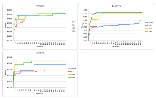
Figure 3.
Overall performance comparison for instances MKP06, MKP35, MKP70 between NPSO and its improvements with classic, modified, and single state Q–Learning. Convergences of the strategies.
Observing the results presented by the distribution Figure 4, it can be again concluded that in general, the standard PSO obtains final results very similar to its version assisted by Q–Learning. With these results and the previously mentioned, we dare say that a possible explanation for this phenomenon would be the high time cost required to train all the action/state pairs of the Q table, causing that, at the end of the execution, the algorithm cannot find a better parametric configuration than the initial one.
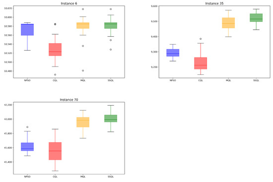
Figure 4.
Overall performance comparison for instances MKP06, MKP35, MKP70 between NPSO and its improvements with classic, modified, and single state Q–Learning. Distributions of the strategies.
This possible problem is mitigated in the other two implemented methods due to the considerable reduction and division of the Q table. Last, the PSO algorithms assisted by the modified Q–Learning and single state Q–Learning obtain significantly better results. Here, we observe that both algorithms, in their runtime, train, and obtain edge configurations adjusted to the instance.
Following up with a robust result review, we employed the two statistical tests (mentioned in Section 5): (a) normality assessment and (b) contrast of hypotheses to determine if the samples come or not from an equidistributed sequence. For determining if observations (runs per instance) draw a Gaussian distribution, we establish as samples follow a normal distribution. Then, is the opposite.
The cutoff of the p–value is , for which results under this threshold state the test is said to be significant ( rejects). Results confirmed that the samples do not follow a normal distribution, so we employ the non-parametric test, Mann–Whitney–Wilcoxon. Here, we assume as the null hypothesis that affirms native methods generate better values than their versions improved by the Q–Learning. Thus, suggests otherwise. In total, six tests were carried out, and the results are presented in Table 7 and Table 8. In the comparison between native PSO and the classic Q–Learning, we can note that the first one exceeds the 95% reliability threshold in 59 of the 70 instances, while the second one only does so in one instance.
Table 7.
Test Wilcoxon–Mann–Whitney for PSO and its enhanced versions solving Instances MKP01–MKP35.
Table 8.
Test Wilcoxon–Mann–Whitney for PSO and its enhanced versions solving Instances MKP36–MKP70.
On the other hand, in the comparison between native PSO and the modified Q–Learning, it is possible to observe that MQL surpasses the threshold in 44 instances, while NPSO does so only in two instances. Regarding the comparison between NPSO and SSQL, we observe that the latter outperforms the threshold in 53 instances, while NPSO does not exceed the threshold in any instance. Finally, in comparing MQL and the single state version, we can analyze that SSQL beats the threshold in 10 instances, while the modified version of Q–Learning only does so in six instances. Furthermore, in the remaining comparisons, MQL and SSQL exceed the 95% confidence threshold in all instances, while classic Q–Learning and NPSO do not exceed the threshold in any instance.
From all obtained results, we can conclude that there is a better performance in the modified Q–Learning and SSQL compared to its classic version and the standard PSO.
7. Conclusions
This article presents an approach to improve the efficiency of a swarm intelligence algorithm when solving complex optimization problems by integrating reinforcement learning techniques. Specifically, we use Q–Learning to adjust the optimal parameters of the particle swarm optimization for solving several instances of the multidimensional knapsack problem.
The analysis of the data obtained in the testing phase shows that the algorithms assisted by reinforcement learning obtained better results in multiple aspects when compared to the native version of PSO. In particular, the single state Q–Learning assisting PSO finds solutions that, as a whole, have better quality in terms of mean, median, standard deviation, and interquartile ranges. In addition, it is observed that SSQL achieves earlier convergence in significant instances when compared to the other methods. Notwithstanding the preceding, it is observed that the native PSO has a slightly better general performance than PSO improved by classic Q–Learning. This is attributed to the high time cost required to train all the action/state pairs. Here, Q–Learning can not guarantee the algorithm finding a better-than-initial parametric configuration at the end of each run. It is suggested to explore the performance of Q–learning with PSO in other optimization problems beyond the multidimensional knapsack problem. In general views, the effect of different parameter settings for the Q–learning algorithm, such as the learning rate and the discount factor, should also be explored to evaluate their effectiveness in the reinforcement learning method in conjunction with PSO.
Finally, it is suggested to explore the comparisons of using the Q–learning method with other bio-inspired algorithms, such as the gray wolf optimizer, whale optimization, bald eagle search optimization, and Harris hawks optimization, among others.
In conclusion, there is a promising approach for improving the performance of swarm intelligence algorithms through reinforcement learning when solving optimization problems. More research is needed to explore its effectiveness in other complex optimization problems and to be able to compare the results obtained with other currently existing methods.
Author Contributions
Formal analysis, R.O., R.S. and B.C.; investigation, R.O., R.S., B.C. and D.N.; methodology, R.O., R.S. and B.C.; resources, R.S. and B.C.; software, R.O. and D.N.; validation, R.S., B.C., V.R., P.O., C.R. and S.M.; writing—original draft, R.O., V.R., P.O., C.R., S.M. and D.N.; writing—review and editing, R.O., R.S., B.C., V.R., P.O., C.R., S.M. and D.N. All authors have read and agreed to the published version of the manuscript.
Funding
Rodrigo Olivares is supported by grant ANID/FONDECYT/INICIACIÓN/11231016. Broderick Crawford is supported by Grant ANID/FONDECYT/REGULAR/1210810.
Data Availability Statement
Data is online available at the following links: https://figshare.com/articles/dataset/Test_Instances/14999907; https://figshare.com/articles/dataset/PSOQLAV_Parameter_Test/14999874; https://figshare.com/articles/dataset/PSOQL_Test_Data/14995374 (accessed on 17 May 2023).
Acknowledgments
Víctor Ríos and Pablo Olivares received scholarships REXE 2286/2022 and REXE 4054/2022, respectively. Both were from Doctorado en Ingeniería Informática Aplicada, Universidad de Valparaíso.
Conflicts of Interest
The authors declare no conflict of interest. The funding sponsors had no role in the study’s design; in the collection, analyses, or interpretation of data; in the writing of the manuscript, and in the decision to publish the results.
References
- Du, K.L.; Swamy, M.; Du, K.L.; Swamy, M. Particle swarm optimization. In Search and Optimization by Metaheuristics: Techniques and Algorithms Inspired by Nature; Springer: Berlin/Heidelberg, Germany, 2016; pp. 153–173. [Google Scholar]
- Talbi, E.G. Metaheuristics: From Design to Implementation; John Wiley & Sons: Hoboken, NJ, USA, 2009. [Google Scholar]
- Boussaïd, I.; Lepagnot, J.; Siarry, P. A survey on optimization metaheuristics. Inf. Sci. 2013, 237, 82–117. [Google Scholar] [CrossRef]
- Panigrahi, B.K.; Shi, Y.; Lim, M.H. Handbook of Swarm Intelligence: Concepts, Principles and Applications; Springer Science & Business Media: Berlin/Heidelberg, Germany, 2011; Volume 8. [Google Scholar]
- Shami, T.M.; El-Saleh, A.A.; Alswaitti, M.; Al-Tashi, Q.; Summakieh, M.A.; Mirjalili, S. Particle Swarm Optimization: A Comprehensive Survey. IEEE Access 2022, 10, 10031–10061. [Google Scholar] [CrossRef]
- Bansal, J.C. Particle swarm optimization. In Evolutionary and Swarm Intelligence Algorithms; Springer: Berlin/Heidelberg, Germany, 2019; pp. 11–23. [Google Scholar]
- Wolpert, D.H.; Macready, W.G. No free lunch theorems for optimization. IEEE Trans. Evol. Comput. 1997, 1, 67–82. [Google Scholar] [CrossRef]
- Hoos, H.H. Automated algorithm configuration and parameter tuning. In Autonomous Search; Springer: Berlin/Heidelberg, Germany, 2012; pp. 37–71. [Google Scholar]
- Huang, C.; Li, Y.; Yao, X. A Survey of Automatic Parameter Tuning Methods for Metaheuristics. IEEE Trans. Evol. Comput. 2019, 24, 201–216. [Google Scholar] [CrossRef]
- Calvet, L.; Armas, J.D.; Masip, D.; Juan, A.A. Learnheuristics: Hybridizing metaheuristics with machine learning for optimization with dynamic inputs. Open Math. 2017, 15, 261–280. [Google Scholar] [CrossRef]
- Sutton, R.S.; Barto, A.G. Reinforcement Learning: An introduction; MIT Press: Cambridge, MA, USA, 2018. [Google Scholar]
- Skackauskas, J.; Kalganova, T. Dynamic Multidimensional Knapsack Problem benchmark datasets. Syst. Soft Comput. 2022, 4, 200041. [Google Scholar] [CrossRef]
- Liu, J.; Wu, C.; Cao, J.; Wang, X.; Teo, K.L. A binary differential search algorithm for the 0–1 multidimensional knapsack problem. Appl. Math. Model. 2016, 40, 9788–9805. [Google Scholar] [CrossRef]
- Cacchiani, V.; Iori, M.; Locatelli, A.; Martello, S. Knapsack problems-An overview of recent advances. Part II: Multiple, multidimensional, and quadratic knapsack problems. Comput. Oper. Res. 2022, 143, 105693. [Google Scholar] [CrossRef]
- Rezoug, A.; Bader-El-Den, M.; Boughaci, D. Application of supervised machine learning methods on the multidimensional knapsack problem. Neural Process. Lett. 2022, 54, 871–890. [Google Scholar] [CrossRef]
- Beasley, J.E. OR-Library: Distributing test problems by electronic mail. J. Oper. Res. Soc. 1990, 41, 1069–1072. [Google Scholar] [CrossRef]
- Liang, Y.C.; Cuevas Juarez, J.R. A self-adaptive virus optimization algorithm for continuous optimization problems. Soft Comput. 2020, 24, 13147–13166. [Google Scholar] [CrossRef]
- Olamaei, J.; Moradi, M.; Kaboodi, T. A new adaptive modified firefly algorithm to solve optimal capacitor placement problem. In Proceedings of the 18th Electric Power Distribution Conference, Kermanshah, Iran, 30 April–1 May 2013; pp. 1–6. [Google Scholar]
- Li, X.; Yin, M. Modified cuckoo search algorithm with self adaptive parameter method. Inf. Sci. 2015, 298, 80–97. [Google Scholar] [CrossRef]
- Li, X.; Yin, M. Self-adaptive constrained artificial bee colony for constrained numerical optimization. Neural Comput. Appl. 2014, 24, 723–734. [Google Scholar] [CrossRef]
- Cui, L.; Li, G.; Zhu, Z.; Wen, Z.; Lu, N.; Lu, J. A novel differential evolution algorithm with a self-adaptation parameter control method by differential evolution. Soft Comput. 2018, 22, 6171–6190. [Google Scholar] [CrossRef]
- de Barros, J.B.; Sampaio, R.C.; Llanos, C.H. An adaptive discrete particle swarm optimization for mapping real-time applications onto network-on-a-chip based MPSoCs. In Proceedings of the 32nd Symposium on Integrated Circuits and Systems Design, Sao Paulo, Brazil, 26–30 August 2019; pp. 1–6. [Google Scholar]
- Cruz-Salinas, A.F.; Perdomo, J.G. Self-adaptation of genetic operators through genetic programming techniques. In Proceedings of the Genetic and Evolutionary Computation Conference, Berlin, Germany, 15–19 July 2017; pp. 913–920. [Google Scholar]
- Kavoosi, M.; Dulebenets, M.A.; Abioye, O.F.; Pasha, J.; Wang, H.; Chi, H. An augmented self-adaptive parameter control in evolutionary computation: A case study for the berth scheduling problem. Adv. Eng. Inform. 2019, 42, 100972. [Google Scholar] [CrossRef]
- Nasser, A.B.; Zamli, K.Z. Parameter free flower algorithm based strategy for pairwise testing. In Proceedings of the 2018 7th international conference on software and computer applications, Kuantan Malaysia, 8–10 February 2018; pp. 46–50. [Google Scholar]
- Zhang, L.; Chen, H.; Wang, W.; Liu, S. Improved Wolf Pack Algorithm for Solving Traveling Salesman Problem. In FSDM; IOS Press: Amsterdam, The Netherlands, 2018; pp. 131–140. [Google Scholar]
- Soto, R.; Crawford, B.; Olivares, R.; Carrasco, C.; Rodriguez-Tello, E.; Castro, C.; Paredes, F.; de la Fuente-Mella, H. A reactive population approach on the dolphin echolocation algorithm for solving cell manufacturing systems. Mathematics 2020, 8, 1389. [Google Scholar] [CrossRef]
- Karimi-Mamaghan, M.; Mohammadi, M.; Meyer, P.; Karimi-Mamaghan, A.M.; Talbi, E.G. Machine learning at the service of meta-heuristics for solving combinatorial optimization problems: A state-of-the-art. Eur. J. Oper. Res. 2022, 296, 393–422. [Google Scholar] [CrossRef]
- Gómez-Rubio, Á.; Soto, R.; Crawford, B.; Jaramillo, A.; Mancilla, D.; Castro, C.; Olivares, R. Applying Parallel and Distributed Models on Bio–Inspired Algorithms via a Clustering Method. Mathematics 2022, 10, 274. [Google Scholar] [CrossRef]
- Caselli, N.; Soto, R.; Crawford, B.; Valdivia, S.; Olivares, R. A self–adaptive cuckoo search algorithm using a machine learning technique. Mathematics 2021, 9, 1840. [Google Scholar] [CrossRef]
- Soto, R.; Crawford, B.; Molina, F.G.; Olivares, R. Human behaviour based optimization supported with self–organizing maps for solving the S–box design Problem. IEEE Access 2021, 2021, 1–14. [Google Scholar] [CrossRef]
- Valdivia, S.; Soto, R.; Crawford, B.; Caselli, N.; Paredes, F.; Castro, C.; Olivares, R. Clustering–based binarization methods applied to the crow search algorithm for 0/1 combinatorial problems. Mathematics 2020, 8, 1070. [Google Scholar] [CrossRef]
- Maturana, J.; Lardeux, F.; Saubion, F. Autonomous operator management for evolutionary algorithms. J. Heuristics 2010, 16, 881–909. [Google Scholar] [CrossRef]
- dos Santos, J.P.Q.; de Melo, J.D.; Neto, A.D.D.; Aloise, D. Reactive search strategies using reinforcement learning, local search algorithms and variable neighborhood search. Expert Syst. Appl. 2014, 41, 4939–4949. [Google Scholar] [CrossRef]
- Zennaki, M.; Ech-Cherif, A. A new machine learning based approach for tuning metaheuristics for the solution of hard combinatorial optimization problems. J. Appl. Sci. 2010, 10, 1991–2000. [Google Scholar] [CrossRef]
- Lessmann, S.; Caserta, M.; Arango, I.M. Tuning metaheuristics: A data mining based approach for particle swarm optimization. Expert Syst. Appl. 2011, 38, 12826–12838. [Google Scholar] [CrossRef]
- Liang, X.; Li, W.; Zhang, Y.; Zhou, M. An adaptive particle swarm optimization method based on clustering. Soft Comput. 2015, 19, 431–448. [Google Scholar] [CrossRef]
- Harrison, K.R.; Ombuki-Berman, B.M.; Engelbrecht, A.P. A parameter-free particle swarm optimization algorithm using performance classifiers. Inf. Sci. 2019, 503, 381–400. [Google Scholar] [CrossRef]
- Dong, W.; Zhou, M. A supervised learning and control method to improve particle swarm optimization algorithms. IEEE Trans. Syst. Man Cybern. Syst. 2016, 47, 1135–1148. [Google Scholar] [CrossRef]
- Kurek, M.; Luk, W. Parametric reconfigurable designs with machine learning optimizer. In Proceedings of the 2012 International Conference on Field-Programmable Technology, Seoul, Republic of Korea, 10–12 December 2012; pp. 109–112. [Google Scholar]
- Al-Duoli, F.; Rabadi, G. Data mining based hybridization of meta-RaPS. Procedia Comput. Sci. 2014, 36, 301–307. [Google Scholar] [CrossRef]
- Wang, G.; Chu, H.E.; Zhang, Y.; Chen, H.; Hu, W.; Li, Y.; Peng, X. Multiple parameter control for ant colony optimization applied to feature selection problem. Neural Comput. Appl. 2015, 26, 1693–1708. [Google Scholar] [CrossRef]
- Seyyedabbasi, A.; Aliyev, R.; Kiani, F.; Gulle, M.U.; Basyildiz, H.; Shah, M.A. Hybrid algorithms based on combining reinforcement learning and metaheuristic methods to solve global optimization problems. Knowl.-Based Syst. 2021, 223, 107044. [Google Scholar] [CrossRef]
- Sadeg, S.; Hamdad, L.; Remache, A.R.; Karech, M.N.; Benatchba, K.; Habbas, Z. Qbso-fs: A reinforcement learning based bee swarm optimization metaheuristic for feature selection. In Proceedings of the Advances in Computational Intelligence: 15th International Work-Conference on Artificial Neural Networks, IWANN 2019, Gran Canaria, Spain, 12–14 June 2019; Proceedings, Part II 15. Springer: Berlin/Heidelberg, Germany, 2019; pp. 785–796. [Google Scholar]
- Sagban, R.; Ku-Mahamud, K.R.; Bakar, M.S.A. Nature-inspired parameter controllers for ACO-based reactive search. Res. J. Appl. Sci. Eng. Technol. 2015, 11, 109–117. [Google Scholar] [CrossRef]
- Nijimbere, D.; Zhao, S.; Gu, X.; Esangbedo, M.O.; Dominique, N. Tabu search guided by reinforcement learning for the max-mean dispersion problem. J. Ind. Manag. Optim. 2020, 17, 3223–3246. [Google Scholar] [CrossRef]
- Reyes-Rubiano, L.; Juan, A.; Bayliss, C.; Panadero, J.; Faulin, J.; Copado, P. A biased-randomized learnheuristic for solving the team orienteering problem with dynamic rewards. Transp. Res. Procedia 2020, 47, 680–687. [Google Scholar] [CrossRef]
- Kusy, M.; Zajdel, R. Stateless Q-learning algorithm for training of radial basis function based neural networks in medical data classification. In Intelligent Systems in Technical and Medical Diagnostics; Springer: Berlin/Heidelberg, Germany, 2014; pp. 267–278. [Google Scholar]
- Eiben, Á.E.; Hinterding, R.; Michalewicz, Z. Parameter control in evolutionary algorithms. IEEE Trans. Evol. Comput. 1999, 3, 124–141. [Google Scholar] [CrossRef]
- Rastegar, R. On the optimal convergence probability of univariate estimation of distribution algorithms. Evol. Comput. 2011, 19, 225–248. [Google Scholar] [CrossRef] [PubMed]
- Skakov, E.S.; Malysh, V.N. Parameter meta-optimization of metaheuristics of solving specific NP-hard facility location problem. J. Phys. Conf. Ser. 2018, 973, 012063. [Google Scholar] [CrossRef]
- López-Ibáñez, M.; Dubois-Lacoste, J.; Cáceres, L.P.; Birattari, M.; Stützle, T. The irace package: Iterated racing for automatic algorithm configuration. Oper. Res. Perspect. 2016, 3, 43–58. [Google Scholar] [CrossRef]
- Soto, R.; Crawford, B.; Olivares, R.; Galleguillos, C.; Castro, C.; Johnson, F.; Paredes, F.; Norero, E. Using autonomous search for solving constraint satisfaction problems via new modern approaches. Swarm Evol. Comput. 2016, 30, 64–77. [Google Scholar] [CrossRef]
- Soto, R.; Crawford, B.; Olivares, R.; Niklander, S.; Johnson, F.; Paredes, F.; Olguín, E. Online control of enumeration strategies via bat algorithm and black hole optimization. Nat. Comput. 2017, 16, 241–257. [Google Scholar] [CrossRef]
- Kaelbling, L.P.; Littman, M.L.; Moore, A.W. Reinforcement learning: A survey. J. Artif. Intell. Res. 1996, 4, 237–285. [Google Scholar] [CrossRef]
- Huotari, T.; Savolainen, J.; Collan, M. Deep Reinforcement Learning Agent for S&P 500 Stock Selection. Axioms 2020, 9, 130. [Google Scholar] [CrossRef]
- Van Otterlo, M.; Wiering, M. Reinforcement learning and markov decision processes. In Reinforcement Learning: State-of-the-Art; Springer: Berlin/Heidelberg, Germany, 2012; pp. 3–42. [Google Scholar]
- Imran, M.; Khushnood, R.A.; Fawad, M. A hybrid data-driven and metaheuristic optimization approach for the compressive strength prediction of high-performance concrete. Case Stud. Constr. Mater. 2023, 18, e01890. [Google Scholar] [CrossRef]
- Watkins, C.J.C.H.; Dayan, P. Q-learning. Mach. Learn. 1992, 8, 279–292. [Google Scholar] [CrossRef]
- Zhang, L.; Tang, L.; Zhang, S.; Wang, Z.; Shen, X.; Zhang, Z. A Self-Adaptive Reinforcement-Exploration Q-Learning Algorithm. Symmetry 2021, 13, 1057. [Google Scholar] [CrossRef]
- Melo, F.S.; Ribeiro, M.I. Convergence of Q-learning with linear function approximation. In Proceedings of the 2007 European Control Conference (ECC), Kos, Greece, 2–5 July 2007; pp. 2671–2678. [Google Scholar]
- Claus, C.; Boutilier, C. The dynamics of reinforcement learning in cooperative multiagent systems. AAAI/IAAI 1998, 1998, 2. [Google Scholar]
- McGlohon, M.; Sen, S. Learning to cooperate in multi-agent systems by combining Q-learning and evolutionary strategy. Int. J. Lateral Comput. 2005, 1, 58–64. [Google Scholar]
- Kennedy, J.; Eberhart, R. Particle swarm optimization. In Proceedings of the ICNN’95-International Conference on Neural Networks, Perth, Australia, 27 November–1 December 1995; Volume 4, pp. 1942–1948. [Google Scholar]
- Piotrowski, A.P.; Napiorkowski, J.J.; Piotrowska, A.E. Population size in Particle Swarm Optimization. Swarm Evol. Comput. 2020, 58, 100718. [Google Scholar] [CrossRef]
- Dammeyer, F.; Voß, S. Dynamic tabu list management using the reverse elimination method. Ann. Oper. Res. 1993, 41, 29–46. [Google Scholar] [CrossRef]
- Drexl, A. A simulated annealing approach to the multiconstraint zero-one knapsack problem. Computing 1988, 40, 1–8. [Google Scholar] [CrossRef]
- Khuri, S.; Bäck, T.; Heitkötter, J. The zero/one multiple knapsack problem and genetic algorithms. In Proceedings of the 1994 ACM Symposium on Applied Computing, New York, NY, USA, 6 April 1994; pp. 188–193. [Google Scholar]
- Crawford, B.; Soto, R.; Astorga, G.; García, J.; Castro, C.; Paredes, F. Putting Continuous Metaheuristics to Work in Binary Search Spaces. Complexity 2017, 2017, 8404231. [Google Scholar] [CrossRef]
- Eberhart, R.C.; Shi, Y. Comparison between genetic algorithms and particle swarm optimization. In Proceedings of the Evolutionary Programming VII: 7th International Conference, EP98, San Diego, CA, USA, 25–27 March 1998; Proceedings 7. Springer: Berlin/Heidelberg, Germany, 1998; pp. 611–616. [Google Scholar]
- Universidad de Valparaíso. Implementations. 2021. Available online: https://figshare.com/articles/dataset/PSOQLAV_Parameter_Test/14999874 (accessed on 27 June 2023).
- Universidad de Valparaíso. Test Instances. 2021. Available online: https://figshare.com/articles/dataset/Test_Instances/14999907 (accessed on 27 June 2023).
- Universidad de Valparaíso. Data and Results. 2021. Available online: https://figshare.com/articles/dataset/PSOQL_Test_Data/14995374 (accessed on 27 June 2023).
Disclaimer/Publisher’s Note: The statements, opinions and data contained in all publications are solely those of the individual author(s) and contributor(s) and not of MDPI and/or the editor(s). MDPI and/or the editor(s) disclaim responsibility for any injury to people or property resulting from any ideas, methods, instructions or products referred to in the content. |
© 2023 by the authors. Licensee MDPI, Basel, Switzerland. This article is an open access article distributed under the terms and conditions of the Creative Commons Attribution (CC BY) license (https://creativecommons.org/licenses/by/4.0/).