Best Proximity Points for p–Cyclic Infimum Summing Contractions

Abstract

We investigate fixed points for p cyclic maps by introducing a new notion of p–cyclic infimum summing maps and a generalized best proximity point for p–cyclic maps. The idea generalizes some results about best proximity points in order to widen the class of sets and maps for which we can ensure the existence and uniqueness of best proximity points. The replacement of the classical notions of best proximity points and distance between the consecutive set arises from the well-known group traveling salesman problem and presents a different approach to solving it. We illustrate the new result with a map that does not satisfy the known results about best proximity maps for p–cyclic maps.

1. Introduction

The Banach contraction principle is a fundamental result in fixed point theory. Fixed point theory is a crucial technique when solving equations of the $Tx=x$ kind for self-mappings $T:A\to A$, defined on subsets of metric or normed spaces. The problem of finding a fixed point $Tx=x$ may be considered a particular case of the optimization task of finding $min\left\{\rho \right(Tx,x):x\in A\}$, where $(X,\rho )$ is a metric space and $T:A\subseteq X\to A$ is a self-map. The problem $min\left\{\rho \right(Tx,x):x\in A\}$ can be investigated for self-maps that lack a fixed point.

The idea to investigate the existence and uniqueness of fixed points for non-self-maps was introduced in [1], where the authors considered the so-called cyclic maps $T\left(A\right)\subseteq B$ and $T\left(B\right)\subseteq A$, where $A,B\subset X$. A non-self-mapping $T:A\to B$ may lack a fixed point. We can alter the fixed points problem $Tx=x$ to the optimization problem $min\left\{\rho \right(Tx,x):x\in A\}$, where $(X,\rho )$ is a metric space and $T:A\cup B\to A\cup B$ be a cyclic map, i.e., we are searching for an element x, which is in some sense closest to $Tx$. The best proximity point results are relevant in this perspective. The notion of a best proximity point was initiated in [2]. A sufficient condition for the uniqueness of the best proximity points in uniformly convex Banach spaces is given in [2]. It turns out that many of the contractive-type conditions that are investigated for fixed points ensure the existence of the best proximity points. Some results of this kind are obtained in [3,4,5,6,7,8,9], which do not even exhaust the publications in the current year 2023. Some other relevant results on the topic can be found in [10,11]. The uniform convexity of the underlying Banach space is replaced by the so called $UC$ and $U{C}^{*}$ properties in [12,13] and the best proximity points’ results are obtained. Connections between uniform convexity, $UC$ and $U{C}^{*}$ properties are investigated in [14].

The optimization problem $min\left\{\rho \right(Tx,x):x\in A\subset X\}$ can be considered as the generalized traveling salesman problem (GTSP) [15,16,17,18,19,20,21,22,23,24,25], which extends the traveling salesperson problem (TSP) [26,27]). Let us recall (TSP). We use a list of cities and distances between each pair of them. What is the shortest possible route that visits each city exactly once and returns to the origin city? Distribute the cities $A_i$, $i=1,\dots ,p$ and $B_j$, $j=1,\dots ,q$ into two sets $A=\{A_i$, $i=1,\dots ,p\}$ and $B=\{B_j$, $j=1,\dots ,q\}$, called clusters. The (GTSP) or group TSP aimed to find the shortest distance $min\{\rho (A_i,B_j):A_i\in A,B_j\in B\}$ (Figure 1).

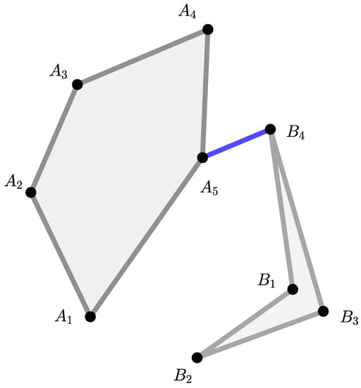
Figure 1. Generalized TSP or group TSP.

This can be interpreted as a problem for three distributes: one collects all the goods produced in the set A and delivers them to a city $A_i$, the second one, whenever they arrive at a city $B_j$, will distribute them in the hole set B, and the third one will transport them from point $A_i$ to point $B_j$. This can be interpreted as two clusters of port at the sea shore, so that there is no a ground route from A to B. The first two distributors are working with trucks and the third one with ships.

We may generalize the above example by replacing the clusters A and B with their convex hulls $\mathrm{conv}A$ and $\mathrm{conv}B$ [18,28,29]. In this case, the following is possible (Figure 2)

$$min\{\rho (a,b):a\in \mathrm{conv}A,b\in \mathrm{conv}B\}<min\{\rho (A_i,B_j):A_i\in A,B_j\in B\}.$$

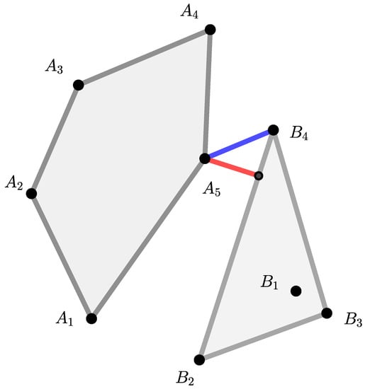
Figure 2. Generalized TSP or group TSP.

If we generalize this problem to p clusters $X_i$, $i=1,\dots ,p$, where each $X_i$ is a convex hull of some points $Y_j^{\left(i\right)}$, $j=1,\dots ,q_i$, we can obtain the following optimization problem:

$$min\{\rho (x_p,x_1)+\sum _{i=1}^{p-1}\rho (x_i,x_{i+1}):x_i\in X_i\},$$

which is not the case for the best proximity points for p–cyclic maps investigated to date, which are introduced in [30].

One illustration of such a model is the widely investigated Unmanned Aerial Vehicle (UAV) and/or unmanned surface vehicle (USV), or UAV and USV simultaneously [31,32,33]. We can consider (Figure 3) that there are four convex sets X, Y, W and Z with sensors, and four UAVs will collect the information. After collecting the data, the UAVs will transfer them to a fifth UAV, so that the path traveled by the fifth UAV should be the shortest.

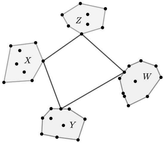
Figure 3. Generalized TSP or group TSP.

A generalization, proposed in [30], is the introduction of p–cyclic maps. This idea have been developed throughout the years [30,34,35]. It is interesting that whenever p–cyclic maps have been considered, using the ideas from [30] the distances between consecutive sets are equal [11,30,34,35]. A new type of condition that warrants the existence and the uniqueness of the best proximity points for sets with different distances between them is presented in [36,37,38,39]. This new type of a map has been called a p–summing map.

It is shown [36] that these new kind of maps are a generalization of the p–cyclic maps introduced in [30,34].

We will show in the next section that a wide class of p–cyclic maps is not covered by the notions introduced in [30] nor in [36], but can be fitted to the convex hull cluster model of the TSP. Therefore, we will present a generalization of the p–summing maps [36], which will cover the p–cyclic contraction maps [30] and p–summing maps [36].

The main goal of the present study is to expand the class of convex sets for which we can solve optimization-type problems with the help of a generalization of the concept of best proximity points.

2. Materials and Methods

In this section, we provide some basic definitions and concepts that are useful and related to the best proximity points. We will denote, using $\mathbb{N}$ and $\mathbb{R}$, the sets of all natural numbers and the set of all real numbers, respectively. We will denote, using $(X,\rho )$ and $(X,\parallel ·\parallel )$, a metric space and a normed space, respectively. We will denote, using $S_X$ and $B_X$, the unit sphere and unit ball, respectively, in the normed space $(X\parallel ·\parallel )$. Let $(X,\rho )$ be a metric space a distance between two subsets $A,B\subset X$, defined by $inf\left\{\rho \right(x-y):x\in A,y\in B\}$ and denoted with $\mathrm{dist}(A,B)$. Whenever we consider a normed space $(X,\parallel ·\parallel )$, we will consider the distance in it to be generated by the norm $\parallel ·\parallel$, i.e., $\rho (x,y)=\parallel x-y\parallel$.

Definition 1

([1,2,30]). Let $A_1,A_2,\dots ,A_p$ be non-empty subsets of an arbitrary set X. A map $T:{\cup }_{i=1}^p{A}_i\to {\cup }_{i=1}^p{A}_i$ is said to be a p–cyclic map if $T\left(A_i\right)\subseteq A_{i+1}$ for $1\le i\le p$, where we use the convention $A_{p+1}=A_1$.

If $p=2$, we obtain the notion of cyclic maps, as introduced in [1]. The notion of best proximity points for cyclic maps was later studied in [2]. The notion of p–cyclic maps for arbitrary p was introduced in [30].

Definition 2

([2,30]). Let $A_1,A_2,\dots ,A_p$ be non-empty subsets of a metric space $(X,\rho )$ and let $T:{\cup }_{i=1}^p{A}_i\to {\cup }_{i=1}^p{A}_i$ be a p–cyclic map. The map T is called a p–cyclic contraction, if for some $k\in (0,1)$, the inequalities

$$\rho (Tx,Ty)\le k\rho (x,y)+(1-k)\mathrm{dist}(A_i,A_{i+1})$$

hold for any $x\in A_i$, $y\in A_{i+1}$ and $1\le i\le p$.

Definition 3

([2,30]). Let $A_1,A_2,\dots ,A_p$ be non-empty subsets of a metric space $(X,\rho )$ and let $T:{\cup }_{i=1}^p{A}_i\to {\cup }_{i=1}^p{A}_i$ be a p–cyclic map. A point $\xi \in A_i$ is said to be the best proximity point of T in $A_i$ if $\rho (\xi ,T\xi )=\mathrm{dist}(A_i,A_{i+1})$.

Definitions 1 and 3 are given for two sets $A_1$ and $A_2$ in [2], and for p–sets in [30].

Definition 4

([40], p. 429). Let $(X,\parallel ·\parallel )$ be a Banach space. The functions ${\delta }_{(X,\parallel ·\parallel )}:[0,2]\to [0,1]$, defined by

$$\begin{array}{ccc}{\delta }_{(X,\parallel ·\parallel )}\left(\epsilon \right)\hfill & =\hfill & inf\left\{1-\frac{\parallel x+y\parallel }{2}:x,y\in B_X,\parallel x-y\parallel \ge \epsilon \right\}\hfill \\ & =\hfill & inf\left\{1-\frac{\parallel x+y\parallel }{2}:x,y\in S_X,\parallel x-y\parallel =\epsilon \right\}\hfill \end{array}$$

are called the modulus of convexity.

Definition 5

([40], p. 429). Let $(X,\parallel ·\parallel )$ be a Banach space. If ${\delta }_{(X,\parallel ·\parallel )}\left(\epsilon \right)>0$ for all $\epsilon \in (0,2]$ the space $(X,\parallel ·\parallel )$ is called uniformly convex.

When there is no danger of misunderstanding, we will use $\delta \left(\epsilon \right)$ instead of ${\delta }_{(X,\parallel ·\parallel )}\left(\epsilon \right)$. It is easy to observe that the inequality ${\displaystyle \delta (\parallel x-y\parallel )\le 1-\frac{\parallel x+y\parallel }{2}}$ holds for any $x,y\in B_X$.

An extensive study of the Geometry of Banach spaces can be found in [40,41,42].

It is proved in [30] that if a map is a p–cyclic contraction and the underlying space $(X,\parallel ·\parallel )$ is a uniformly convex Banach space, then it has best proximity points for every set $A_i$, $1\le i\le p$. Let $(X,\rho )$ be a metric space and $A_i\subset X$, $i=1,\dots ,p$. We denote

$$P(A_1,\dots ,A_p)=\sum _{i=1}^p\mathrm{dist}(A_i,A_{i+1}),$$

where we use the convention $A_{p+1}=A_1$.

We will use the notation $P=P(A_1,\dots ,A_p)$ to fit some of the formulas into the text field.

Definition 6

([36]). Let $A_i$, $i=1,\dots ,p$ be subsets of a metric space $(X,\rho )$. A map $T:{\cup }_{i=1}^p{A}_i\to {\cup }_{i=1}^p{A}_i$ will be called a p–cyclic summing contraction if it is a p–cyclic map and there exists $k\in (0,1)$, such that, for any $x_i\in A_i$, $i=1,\dots ,p$ there holds the inequality

$$\sum _{i=1}^{p-1}\rho (T{x}_i,T{x}_{i+1})+\rho (T{x}_p,T{x}_1)\le k\left(\sum _{i=1}^{p-1}\rho (x_i,x_{i+1})+\rho (x_p,x_1)\right)+(1-k)P.$$

(1)

Whenever we consider a p–cyclic contraction [30] or a p–cyclic summing contraction [36] and the underlying space $(X,\parallel ·\parallel )$ be a uniformly convex Banach space, it follows that the if $\xi$ is the best proximity point of T in $A_i$; therefore, $T\xi$ is the best proximity point of T in $A_{i+1}$.

Let us consider an example illustrated in Figure 4. Let $T:{\cup }_{i=1}^3{A}_i\to {\cup }_{i=1}^3{A}_i$ be a 3–cyclic map. If T is a p–cyclic contraction, then $\mathrm{dist}(A_1,A_2)=\mathrm{dist}(A_2,A_3)=\mathrm{dist}(A_3,A_1)$ [30].

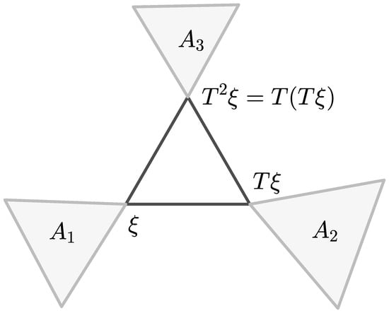
Figure 4. A p–cyclic contraction.

Let us consider an example illustrated in Figure 5. Let $T:{\cup }_{i=1}^3{A}_i\to {\cup }_{i=1}^3{A}_i$. If T is a 3–cyclic contraction, then, according to [30], $\mathrm{dist}(A_1,A_2)=\mathrm{dist}(A_2,A_3)=\mathrm{dist}(A_3,A_1)$ should hold, which is not the case. If there is a p–cyclic summing contraction, then it is possible to construct map T [36].

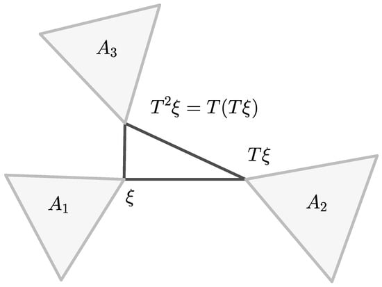
Figure 5. A p–cyclic summing contraction.

Let us consider an example illustrated in Figure 6. Let $T:{\cup }_{i=1}^3{A}_i\to {\cup }_{i=1}^3{A}_i$ be a 3–cyclic map. We see that $\xi$ is a best proximity point of T in $A_1$, i.e., $\rho (\xi ,T\xi )=\mathrm{dist}(A_1,A_2)$, but $T\xi$ is not a best proximity point of T in $A_2$, i.e., $\rho (T\xi ,T^2\xi )>\rho (\eta ,T\eta )=\mathrm{dist}(A_2,A_3)$. This example shows that in order to obtain the best proximity point results for p–cyclic maps, it is not sufficient to construct a specific p–cyclic maps for arbitrary positioned subsets in the space $(X,\rho )$, but the positioning of the sets $A_i$ in the underlying space is crucial.

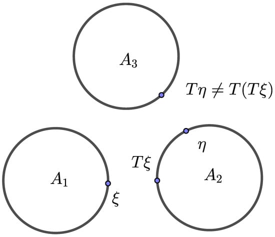
Figure 6. A p–cyclic summing contraction.

We will try to provide a contractive condition so that $\rho (\xi ,T\xi )+\rho (T\xi ,T^2\xi )+\rho (T^2\xi ,T^3\xi )$ is equal to a constant depending on the sets $A_i$, $i=1,\dots ,p$, for a unique $\xi \in A_1$, to hold $\xi =T^3\xi$, and whenever the sets are of the kind from Figure 4 or Figure 5, the investigated mapscoincide with the p–cyclic contractions or p–cyclic summing contractions, i.e., in this case, the point $\xi \in A_i$ is a best proximity point of T in $A_i$ in the sense of [2,30].

The next two lemmas, established in [2], are crucial in the investigation of best proximity points for p–cyclic maps.

Lemma 1

([2]). Let $(X,\parallel ·\parallel )$ be a uniformly convex Banach space. Let $A\subset X$ be a non-empty, closed, convex subset, and $B\subset X$ be a non-empty, closed subset. Let ${\left\{x_n\right\}}_{n=1}^{\infty }$ and ${\left\{z_n\right\}}_{n=1}^{\infty }$ be sequences in A and ${\left\{y_n\right\}}_{n=1}^{\infty }$ be a sequence in B satisfying

1. 

${\displaystyle \underset{n\to \infty }{lim}\parallel z_n-y_n\parallel =\mathrm{dist}(A,B)}$

2. 

for every $\epsilon >0$ there exists $N_0\in \mathbb{N}$, such that for all $m>n\ge N_0$,

$$\parallel x_m-y_n\parallel \le \mathrm{dist}(A,B)+\epsilon .$$

Then for every $\epsilon >0$, there exists $N_1\in \mathbb{N}$, such that for all $m>n>N_1$, holds $\parallel x_m-z_n\parallel \le \epsilon$.

Lemma 2

([2]). Let $(X,\parallel ·\parallel )$ be a uniformly convex Banach space. Let $A\subset X$ be a non-empty, closed, convex subset, and $B\subset X$ be a non-empty, closed subset. Let ${\left\{x_n\right\}}_{n=1}^{\infty }$ and ${\left\{z_n\right\}}_{n=1}^{\infty }$ be sequences in A and ${\left\{y_n\right\}}_{n=1}^{\infty }$ be a sequence in B satisfying

1. 

${\displaystyle \underset{n\to \infty }{lim}\parallel x_n-y_n\parallel =\mathrm{dist}(A,B)}$

2. 

${\displaystyle \underset{n\to \infty }{lim}\parallel z_n-y_n\parallel =\mathrm{dist}(A,B)}$.

Then ${\displaystyle \underset{n\to \infty }{lim}\parallel x_n-z_n\parallel =0}$.

We will use the well-known inequality, which is a corollary of the triangle inequality for the metric function $\rho (·,·)$.

Lemma 3

([43], p. 3). Let $(X,\rho )$ be a metric space and $a,b,c\in X$. Then,

$$\rho (a,b)\ge \rho (a,c)-\rho (c,b).$$

3. Results

Let $(X,\rho )$ be a metric space and $A_i\subset X$, $i=1,\dots ,p$. We denote

$$S\left({\left\{x_i\right\}}_{i=1}^p\right)=\sum _{i=1}^p\rho (x_i,x_{i+1})=\rho (x_p,x_1)+\sum _{i=1}^{p-1}\rho (x_i,x_{i+1}),$$

where $x_i\in A_i$, $i=1,\dots ,p+1$ and we use the convention $A_{p+1}=A_1$ and $x_{p+1}=x_1$.

Whenever we consider the sets $A_i\subset X$, $i=1,\dots ,p$ we will assume that we consider them as an ordered p–tuple $(A_1,\dots ,A_p)$.

If it is more convenient for the reader, we will use the notation

$$S(x_1,\dots ,x_p)=S\left({\left\{x_i\right\}}_{i=1}^p\right).$$

Definition 7.

Let $(X,\rho )$ be a metric space and $A_i\subset X$, $i=1,\dots ,p$. Let us denote

$$D(A_1,A_2,\dots ,A_p)=inf\{S(x_1,\dots ,x_p):x_i\in A_i,i=1,\dots ,p\}.$$

We will call $D(A_1,A_2,\dots ,A_p)$ a distance between the sets $A_1,\dots ,A_p$ in the order $(A_1,A_2,\dots ,A_p)$.

If we consider 4 sets $(A_1,A_2,A_3,A_4)$ (Figure 7), then $D(A_1,A_2,A_3,A_4)$ is the infimum of the perimeter of the quadrilateral $x_1{x}_2{x}_3{x}_4$.

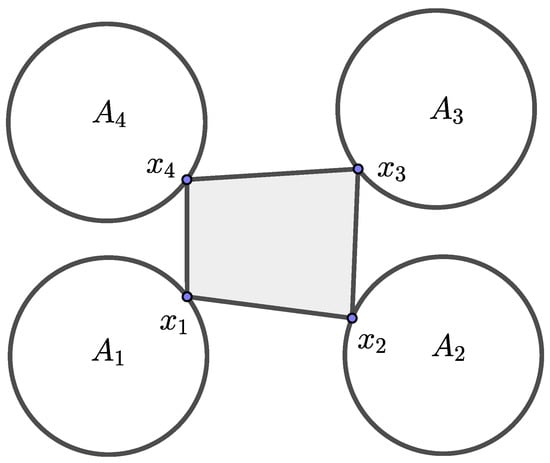
Figure 7. The infimum perimeter of the quadrilateral $x_1{x}_2{x}_3{x}_4$.

We will use the notation $D=D(A_1,A_2,\dots ,A_p)$ to fit some of the formulas into the text field.

Definition 8.

Let $A_1,A_2,\dots ,A_p$ be non-empty subsets of a metric space $(X,\rho )$ and let $T:{\cup }_{i=1}^p{A}_i\to {\cup }_{i=1}^p{A}_i$ be a p–cyclic map. A point $\xi \in A_i$ is said to be a generalized best proximity point of T in $A_i$ if $S(\xi ,T\xi ,\dots ,T^{p-1}\xi )=D(A_1,\dots ,A_p)$.

There holds $D(A_1,\dots ,A_p)=D(A_i,A_{i+1},\dots ,A_p,A_1,\dots ,A_{i-1})$.

A crucial element in the investigation of best proximity points is the iterated sequence ${\left\{x_n\right\}}_{n=1}^{\infty }$. For an arbitrary chosen $x_0\in A_i$, we define $x_1=T{x}_0$. If we have already defined $x_n$, then we use $x_{n+1}=T{x}_n$. Without loss of generality, we can assume that $x_0\in A_1$, as long as we can always enumerate the sets $A_i$ so that $x_0\in A_1$.

Let $(X,\rho )$ be a metric space and $A_i\subset X$ where $i=1,\dots ,p$. Let ${\left\{x_i\right\}}_{i=1}^p$ and ${\left\{y_i\right\}}_{i=1}^p$ be such that $x_i,y_i\in A_i$ for $i=1,\dots ,p$. Let us denote

$$S\left({\left\{x_i\right\}}_{i=1}^p,{\left\{y_i\right\}}_{i=1}^p\right)=\sum _{i=1}^p\rho (x_i,y_{i+1})=\rho (x_p,y_1)+\sum _{i=1}^{p-1}\rho (x_i,y_{i+1}),$$

using the convention $y_{p+1}=y_1$.

With the following definitions, we will establish the concept of a p–cyclic infimum summing contraction.

Definition 9.

Let $(X,\rho )$ be a metric space and $A_i\subset X$, $i=1,\dots ,p$. Let $T:{\cup }_{i=1}^p{A}_i\to {\cup }_{i=1}^p{A}_i$ be a p–cyclic map. We say that T is a p–cyclic infimum summing contraction if, for any $a_i,b_i\in A_i$, the inequality

$$S\left({\left\{T{a}_i\right\}}_{i=1}^p,{\left\{T{b}_i\right\}}_{i=1}^p\right)\le \lambda S\left({\left\{a_i\right\}}_{i=1}^p,{\left\{b_i\right\}}_{i=1}^p\right)+(1-\lambda )D(A_1,\dots A_p)$$

(2)

holds for some $\lambda \in [0,1)$.

Sometimes, it will be easier to apply (2) in the form

$$S\left({\left\{T{a}_i\right\}}_{i=1}^p,{\left\{T{b}_i\right\}}_{i=1}^p\right)-D\le \lambda \left(S\left({\left\{a_i\right\}}_{i=1}^p,{\left\{b_i\right\}}_{i=1}^p\right)-D\right).$$

(3)

Theorem 1.

Let $(X,\parallel ·\parallel )$ be a uniformly convex Banach space, and let $A_i\subset X$, $i=1,\dots ,p$ and $T:{\cup }_{i=1}^p{A}_i\to {\cup }_{i=1}^p{A}_i$ be a p–cyclic infimum summing contraction. Then:

1. 

There exists ${\alpha }^i\in A_i$, $i=1,\dots ,p$, such that for each arbitrarily chosen $a^i\in A_i$, $i=1,\dots ,p$ there holds

$$\underset{n\to \infty }{lim}{T}^{pn}{a}^i={\alpha }^i.$$

2. 

${\alpha }^i$ is a unique fixed point of $T^p$ in $A_i$ for every $i=1,\dots ,p$.

3. 

${\alpha }_{i+1}=T{\alpha }_i$ for every $i=1,\dots ,p$, where we use the convention ${\alpha }_{p+1}={\alpha }_1$.

4. 

$S({\alpha }^1,\dots ,{\alpha }^k)=D(A_1,\dots ,A_p)$, i.e., ${\alpha }^i$ is a generalized best proximity point of T in $A_i$.

4. Auxiliary Results

We will prove some auxiliary results that will be needed for the proof of Theorem 1.

Lemma 4.

Let $(X,\rho )$ be a metric space and $A_i\subset X$, $i=1,\dots ,p$. Let $T:{\bigcup }_{i=1}^p{A}_i\to {\bigcup }_{i=1}^p{A}_i$ be a p–cyclic infimum summing contraction and let $a_i,b_i\in A_i$ for $i=1,\dots ,p$ be arbitrarily chosen. Then, the following inequality

$$S\left({\left\{T^{pn}{a}_i\right\}}_{i=1}^p,{\left\{T^{pn}{b}_i\right\}}_{i=1}^p\right)\le {\lambda }^{pn}S\left({\left\{a_i\right\}}_{i=1}^p,{\left\{b_i\right\}}_{i=1}^p\right)+(1-{\lambda }^{pn})D(A_1,\dots ,A_p)$$

(4)

holds for all arbitrary chosen $a_i,b_i\in A_i$.

Proof. 

By applying (2) three times, we can obtain the chain of inequalities

$$\begin{array}{ccc}S\left({\left\{T^{pn}{a}_i\right\}}_{i=1}^p,{\left\{T^{pn}{b}_i\right\}}_{i=1}^p\right)-D\hfill & \le \hfill & {\displaystyle \lambda (S\left({\left\{T^{pn-1}{a}_i\right\}}_{i=1}^p,{\left\{T^{pn-1}{b}_i\right\}}_{i=1}^p\right)-D)}\hfill \\ & \le \hfill & {\displaystyle {\lambda }^2(S\left({\left\{T^{pn-2}{a}_i\right\}}_{i=1}^p,{\left\{T^{pn-2}{b}_i\right\}}_{i=1}^p\right)-D)}\hfill \\ & \le \hfill & {\displaystyle {\lambda }^3(S\left({\left\{T^{pn-3}{a}_i\right\}}_{i=1}^p,{\left\{T^{pn-3}{b}_i\right\}}_{i=1}^p\right)-D)}\hfill \\ & & \dots \dots \dots \dots \dots \dots \dots \hfill \\ & \le \hfill & {\displaystyle {\lambda }^{pn}(S\left({\left\{a_i\right\}}_{i=1}^p,{\left\{b_i\right\}}_{i=1}^p\right)-D).}\hfill \end{array}$$

□

Corollary 1.

Let $(X,\rho )$ be a metric space and $A_i\subset X$, $i=1,\dots ,p$. Let $T:{\cup }_{i=1}^p{A}_i\to {\cup }_{i=1}^p{A}_i$ be a p–cyclic infimum summing contraction and $x\in {\bigcup }_{i=1}^p{A}_i$ be arbitrarily chosen. Then, the inequalities

$$S\left({\left\{T^{(n+m+i)}x\right\}}_{i=0}^{p-1}\right)\le {\lambda }^{n}S\left({\left\{T^{(m+i)}x\right\}}_{i=0}^{p-1}\right)+(1-{\lambda }^n)D(A,\dots ,A_p)$$

(5)

and

$$S(T^{(n+1)p}x,T^{p+1}x,T^{p+2}x,\dots ,T^{2p-1}x)\le {\lambda }^{p}S(T^{np}x,Tx,T^{2}x,\dots ,T^{p-1}x)+(1-{\lambda }^p)Dhold.$$

(6)

Lemma 5.

Let $(X,\rho )$ be a metric space, $A_i\subset X$, $i=1,\dots ,p$ be nonempty convex subsets. Let $T:{\cup }_{i=1}^p{A}_i\to {\cup }_{i=1}^p{A}_i$ be a p–cyclic infimum summing contraction. Then, for every $x\in {\cup }_{i=1}^p{A}_i$, the sequence ${\left\{T^{pn}x\right\}}_{n=0}^{\infty }$ is a bounded one.

Proof. 

Without loss of generality, we can assume that $x\in A_1$. From (6), it follows that

$$S(T^{(n+1)p}x,T^{p+1}x,T^{p+2}x,\dots ,T^{2p-1}x)\le {\lambda }^{p}S(T^{np}x,Tx,T^{2}x,\dots ,T^{p-1}x)+(1-{\lambda }^p)D,$$

i.e.,

$$\begin{array}{ccc}{S}_1\hfill & =\hfill & {\displaystyle \rho (T^{(n+1)p}x,T^{p+1}x)+\rho (T^{(n+1)p}x,T^{2p-1}x)+\sum _{i=1}^{p-2}\rho (T^{p+i}x,T^{p+i+1}x)}\hfill \\ \hfill & \le \hfill & {\displaystyle {\lambda }^p(\rho (T^{np}x,T^{1}x)+\rho (T^{np}x,T^{p-1}x)+\sum _{i=1}^{p-2}\rho (T^{i}x,T^{i+1}x))+(1-{\lambda }^p)D.}\hfill \end{array}$$

(7)

From Lemma 3, we have

$$\begin{array}{c}\rho (T^{p+i}x,T^{p+i+1}x)\ge \rho (T^{p+i}x,T^{i+1}x)-\rho (T^{i+1}x,T^{p+i+1}x)\\ \rho (T^{p+i}x,T^{i+1}x)\ge \rho (T^{i+1}x,T^{i}x)-\rho (T^{i}x,T^{p+i}x),\end{array}$$

(8)

i.e.,

$$\rho (T^{p+i}x,T^{p+i+1}x)\ge \rho (T^{i+1}x,T^{i}x)-\rho (T^{i}x,T^{p+i}x)-\rho (T^{i+1}x,T^{p+i+1}x)$$

(9)

and

$$\begin{array}{c}\rho (T^{(n+1)p}x,T^{p+1}x)\ge \rho (T^{(n+1)p}x,Tx)-\rho (Tx,T^{p+1}x)\\ \rho (T^{(n+1)p}x,T^{2p-1}x)\ge \rho (T^{(n+1)p}x,T^{p-1}x)-\rho (T^{p-1}x,T^{2p-1}x).\end{array}$$

(10)

Let us put ${\displaystyle C=2\sum _{i=1}^{p-1}\rho (T^{p+i}x,T^{i}x)}$. From (7), (9) and (10); it follows that

$$\begin{array}{ccc}{S}_2\hfill & =\hfill & {\displaystyle \rho (T^{(n+1)p}x,Tx)+\rho (T^{(n+1)p}x,T^{p-1}x)+\sum _{i=1}^{p-2}\rho (T^{i}x,T^{i+1}x)-C}\hfill \\ & \le \hfill & {\displaystyle {\lambda }^p(\rho (T^{np}x,Tx)+\rho (T^{np}x,T^{p-1}x)+\sum _{i=1}^{p-2}\rho (T^{i}x,T^{i+1}x))+(1-{\lambda }^p)D,}\hfill \end{array}$$

i.e.,

$$S(T^{(n+1)p}x,Tx,T^{2}x,\dots ,T^{p-1}x)\le {\lambda }^{p}S(T^{np}x,Tx,T^{2}x,\dots ,T^{p-1}x)+(1-{\lambda }^p)D+C.$$

(11)

By applying (11) $n-1$ times, we can obtain the chain of inequalities

$$\begin{array}{ccc}{S}_3\hfill & =\hfill & {\displaystyle S(T^{np}x,Tx,T^{2}x,\dots ,T^{p-1}x)}\hfill \\ \hfill & \le \hfill & {\displaystyle {\lambda }^{p}S(T^{(n-1)p}x,Tx,T^{2}x,\dots ,T^{p-1}x)+(1-{\lambda }^p)D+C}\hfill \\ \hfill & \le \hfill & {\displaystyle {\lambda }^{2p}S(T^{(n-2)p}x,Tx,T^{2}x,\dots ,T^{p-1}x)+(1-{\lambda }^{2p})D+C+{\lambda }^{2p}C}\hfill \\ \hfill & \le \hfill & {\displaystyle {\lambda }^{3p}S(T^{(n-3)p}x,Tx,T^{2}x,\dots ,T^{p-1}x)+(1-{\lambda }^{3p})D+C+{\lambda }^{2p}C+{\lambda }^{3p}C}\hfill \\ \hfill & \hfill & \dots \dots \dots \dots \dots \dots \dots \dots \dots \dots \dots \hfill \\ \hfill & \le \hfill & {\displaystyle {\lambda }^{(n-1)p}S(T^{p}x,Tx,T^{2}x,\dots ,T^{p-1}x)+(1-{\lambda }^{(n-1)p})D+C\frac{1-{\lambda }^{(n-1)p}}{1-{\lambda }^p}}\hfill \\ \hfill & \le \hfill & {\displaystyle S(T^{p}x,Tx,T^{2}x,\dots ,T^{p-1}x)+C\frac{1}{1-{\lambda }^p}.}\hfill \end{array}$$

(12)

From the definition of the function S, we can obtain

$$S(T^{np}x,Tx,T^{2}x,\dots ,T^{p-1}x)=\rho (T^{np}x,Tx)+\rho (T^{np}x,T^{p-1}x)+\sum _{i=1}^{p-2}\rho (T^{i}x,T^{i+1}x)$$

and

$$S(T^{p}x,Tx,T^{2}x,\dots ,T^{p-1}x)=\rho (T^{p}x,Tx)+\sum _{i=1}^{p-1}\rho (T^{i}x,T^{i+1}x).$$

Consequently, by (12), we obtain the inequality

$${\displaystyle \rho (T^{np}x,T^{1}x)+\rho (T^{np}x,T^{p-1}x)\le \rho (T^{p}x,Tx)+\rho (T^{p}x,T^{p-1}x)+C\frac{1}{1-{\lambda }^p}.}$$

(13)

As far as $\rho (T^{p}x,Tx)+\rho (T^{p}x,T^{p-1}x)+C\frac{1}{1-{\lambda }^p}$ does not depend on n, it follows that the sequence ${\left\{T^{pn}x\right\}}_{n=1}^{\infty }$ is a bounded one. □

Let $(X,\rho )$ be a metric space and $x_i,y_i\in X$, where $i=1,\dots ,p$. Let us use the notations

$$s\left(x_1,y_1,{\left\{x_i\right\}}_{i=2}^p,{\left\{y_i\right\}}_{i=2}^p\right)=S\left({\left\{x_i\right\}}_{i=1}^p,{\left\{y_i\right\}}_{i=1}^p\right)=\rho (x_p,y_1)+\sum _{i=1}^{p-1}\rho (x_i,y_{i+1})$$

and

$$s\left(x_1,y_1,{\left\{x_i\right\}}_{i=2}^p\right)=s\left(x_1,y_1,{\left\{x_i\right\}}_{i=2}^p,{\left\{x_i\right\}}_{i=2}^p\right).$$

Lemma 6.

Let $(X,\rho )$ be a metric space and $A_i\subset X$, where $i=1,\dots ,p$. Let $\epsilon >0$ and there are $x,y\in A_1$, $a_i\in A_i$ for $i=1,\dots ,p$, such that the inequality

$$max\left\{s\left(x,y,{\left\{a_i\right\}}_{i=2}^p\right),s\left(y,x,{\left\{a_i\right\}}_{i=2}^p\right)\right\}\le D(A_1,\dots ,A_p)+\epsilon$$

holds true. Then, there holds

$$D(A_1,\dots ,A_p)-\epsilon \le min\left\{s\left(x,y,{\left\{a_i\right\}}_{i=2}^p\right),s\left(y,x,{\left\{a_i\right\}}_{i=2}^p\right)\right\}.$$

Proof. 

From the definition of $D(A_1,\dots ,A_p)$, it follows that

$$D(A_1,\dots ,A_p)\le S(x,a_2,a_3,\dots ,a_p)\mathrm{and}D(A_1,\dots ,A_p)\le S(y,a_2,a_3,\dots ,a_p),$$

(14)

i.e.,

$$S(x,a_2,a_3,\dots ,a_p)+S(y,a_2,a_3,\dots ,a_p)\ge 2D(A_1,\dots ,A_p).$$

(15)

Let us put $s\left(x\right)=s\left(x,y,{\left\{a_i\right\}}_{i=2}^p\right)$ and $s\left(y\right)=s\left(y,x,{\left\{a_i\right\}}_{i=2}^p\right)$. Using the introduced notations, we have

$$s\left(x\right)=s\left(x,y,{\left\{a_i\right\}}_{i=2}^p\right)=\rho (x,a_2)+\rho (y,a_p)+\sum _{i=2}^{p-1}\rho (a_i,a_{i+1})$$

and

$$s\left(y\right)=s\left(y,x,{\left\{a_i\right\}}_{i=2}^p\right)=\rho (y,a_2)+\rho (x,a_p)+\sum _{i=2}^{p-1}\rho (a_i,a_{i+1}).$$

It is easy to observe that

$$\begin{array}{ccc}s\left(x\right)+s\left(y\right)\hfill & =\hfill & {\displaystyle \left(\rho (x,a_2)+\rho (y,a_k)+\sum _{i=2}^{p-1}\rho (a_i,a_{i+1})\right)}\hfill \\ \hfill & \hfill & +\left({\displaystyle \rho (y,a_2)+\rho (x,a_k)+\sum _{i=2}^{p-1}\rho (a_i,a_{i+1})}\right)\hfill \\ \hfill & =\hfill & {\displaystyle \left(\rho (x,a_2)+\rho (x,a_k)+\sum _{i=2}^{p-1}\rho (a_i,a_{i+1})\right)}\hfill \\ \hfill & \hfill & +\left({\displaystyle \rho (y,a_2)+\rho (y,a_k)+\sum _{i=2}^{p-1}\rho (a_i,a_{i+1})}\right)\hfill \\ \hfill & =\hfill & S(x,a_2,a_3,\dots ,a_p)+S(y,a_2,a_3,\dots ,a_p)\ge 2D(A_1,\dots ,A_p).\hfill \end{array}$$

(16)

Let us assume that

$$s\left(y\right)<D(A_1,\dots ,A_p)-\epsilon ,$$

(17)

then, from (16), it follows that $s\left(x\right)>D(A_1,\dots ,A_p)+\epsilon$, which is a contradiction, and thus $s\left(x\right)>D(A_1,\dots ,A_p)-\epsilon$.

Using similar arguments, we can obtain that $s\left(y\right)>D(A_1,\dots ,A_p)-\epsilon$. □

Lemmas 1 and 2 of Eldred and Veeramani are crucial in obtaining results about the best proximity points. We will need generalizations of these lemmas in order to obtain similar results about p–cyclic infimum summing contraction maps.

Lemma 7

(a generalization of Lemma 1). Let $(X,\parallel ·\parallel )$ be a uniformly convex Banach space, $A_i\subset X$$i=1,\dots ,p$ and $A_1$ be a convex set. Let ${\left\{{\alpha }_n\right\}}_{n=1}^{\infty },{\left\{{\beta }_n\right\}}_{n=1}^{\infty }\subset A_1$ and ${\left\{a_n^i\right\}}_{n=1}^{\infty }\subset A_i$ for $i=2,\dots ,p$. If there hold

$$\begin{array}{c}{\displaystyle \underset{n\to \infty }{lim}s\left({\alpha }_n,{\beta }_n,{\left\{a_n^i\right\}}_{i=2}^p\right)=D(A_1,\dots ,A_p)}\hfill \\ {\displaystyle \underset{n\to \infty }{lim}s\left({\beta }_n,{\alpha }_n,{\left\{a_n^i\right\}}_{i=2}^p\right)=D(A_1,\dots ,A_p)}\hfill \end{array}$$

(18)

then ${lim}_{n\to \infty }(\parallel {\alpha }_n-{\beta }_n\parallel )=0$.

Proof. 

From (16), we have the equality

$$s\left({\alpha }_n,{\beta }_n,{\left\{a_n^i\right\}}_{i=2}^p\right)+s\left({\beta }_n,{\alpha }_n,{\left\{a_n^i\right\}}_{i=2}^p\right)=S({\alpha }_n,a_n^2,\dots ,a_n^k)+S({\beta }_n,a_n^2,\dots ,a_n^k).$$

(19)

By (18) and (19), we can obtain that

$$\underset{n\to \infty }{lim}\left(S\left({\alpha }_n,a_n^2,\dots ,a_n^p\right)+S\left({\beta }_n,a_n^2,\dots ,a_n^p\right)\right)=2D(A_1,\dots ,A_p).$$

(20)

From the definition of $D(A_1,\dots ,A_p)$, it follows

$$D(A_1,\dots ,A_p)\le S\left({\alpha }_n,a_n^2,\dots ,a_n^p\right)andD(A_1,\dots ,A_p)\le S\left({\beta }_n,a_n^2,\dots ,a_n^p\right).$$

(21)

Now, using (20) and (21), we can obtain

$$\underset{n\to \infty }{lim}S\left({\alpha }_n,a_n^2,\dots ,a_n^k\right)=D(A_1,\dots ,A_p)$$

and

$$\underset{n\to \infty }{lim}S\left({\beta }_n,a_n^2,\dots ,a_n^k\right)=D(A_1,\dots ,A_p).$$

Consequently, there is $M<+\infty$, so that

$$M=\underset{n\in \mathbb{N}}{sup}\left\{max(\parallel {\alpha }_n-a_n^2\parallel ,\parallel {\beta }_n-a_n^2\parallel ,\parallel {\alpha }_n-a_n^p\parallel ,\parallel {\beta }_n-a_n^p\parallel )\right\}.$$

Let us assume that ${lim}_{n\to \infty }(\parallel {\alpha }_n-{\beta }_n\parallel )=0$ is not true. Then, there exists $\epsilon >0$, such that, for any $N\in \mathbb{N}$, there is $m>N$, so that the inequality $∥{\alpha }_m-{\beta }_m∥>\epsilon$ holds true.

We have that, for every $w\in X$, the following is valid

$${\displaystyle 2max\{\parallel {\alpha }_m-w\parallel ,\parallel {\beta }_m-w\parallel \}\ge \parallel {\alpha }_m-w\parallel +\parallel {\beta }_m-w\parallel \ge \parallel {\alpha }_m-{\beta }_m\parallel >\epsilon .}$$

Thus, following the definition of M, it follows that, for every $q_m\in \{a_m^2,a_m^p\}$ holds

$${\displaystyle \frac{\epsilon }{2}\le max\{\parallel {\alpha }_m-q_m\parallel ,\parallel {\beta }_m-q_m\parallel \}\le M.}$$

Using that ${\delta }_{\parallel ·\parallel }$ is an increasing function and the uniform convexity of $(X,\parallel ·\parallel )$, it follows that there is ${\displaystyle \delta =\frac{\epsilon }{2}{\delta }_{\parallel ·\parallel }\left(\frac{\epsilon }{M}\right)>0}$, such that

$$∥\frac{({\alpha }_m-a_m^2)+({\beta }_m-a_m^2)}{2}∥\le max\{\parallel {\alpha }_m-a_m^2\parallel ,\parallel {\beta }_m-a_m^2\parallel \}-\delta$$

and

$$∥\frac{({\alpha }_m-a_m^p)+({\beta }_m-a_m^p)}{2}∥\le max\{\parallel {\alpha }_m-a_m^p\parallel ,\parallel {\beta }_m-a_m^p\parallel \}-\delta .$$

Thus,

$$\begin{array}{ccc}{S}_4\hfill & =\hfill & S\left(\frac{{\alpha }_m+{\beta }_m}{2},a_m^2,\dots ,a_m^p\right)\hfill \\ \hfill & =\hfill & {\displaystyle ∥\frac{{\alpha }_m+{\beta }_m}{2}-a_m^2∥+∥\frac{{\alpha }_m+{\beta }_m}{2}-a_m^p∥+\sum _{i=2}^{p-1}\parallel a_m^i-a_m^{i+1}\parallel }\hfill \\ \hfill & \le \hfill & {\displaystyle max\{\parallel {\alpha }_m-a_m^1\parallel ,\parallel {\beta }_m-a_m^1\parallel \}+max\{\parallel {\alpha }_m-a_m^p\parallel ,\parallel {\beta }_m-a_m^p\parallel \}}\hfill \\ \hfill & \hfill & {\displaystyle +\sum _{i=2}^{p-1}\parallel a_m^i-a_m^{i+1}\parallel -2\delta .}\hfill \end{array}$$

(22)

Let us put $x_m=\left({\alpha }_m,{\beta }_m,{\left\{a_m^i\right\}}_{i=2}^p\right)$ and $y_m=\left({\beta }_m,{\alpha }_m,{\left\{a_m^i\right\}}_{i=2}^p\right)$. From the equality

$$\begin{array}{ccc}{S}_5\left(m\right)\hfill & =\hfill & max\left\{∥{\alpha }_m-a_m^1∥,∥{\beta }_m-a_m^1∥\right\}+max\{\parallel {\alpha }_m-a_m^p\parallel ,\parallel {\beta }_m-a_m^p\parallel \}\hfill \\ & & {\displaystyle +\sum _{i=2}^{p-1}\parallel a_m^i-a_m^{i+1}\parallel }\hfill \\ & =\hfill & max\left\{s\left(x_m\right),s\left(y_m\right),S({\alpha }_m,a_m^2,\dots ,a_m^p),S({\beta }_m,a_m^2,\dots ,a_m^p)\right\}\hfill \end{array}$$

it follows that

$$\underset{n\to \infty }{lim}{S}_5\left(m\right)=D.$$

(23)

Therefore, from (22) and (23), for a sufficiently large $m\in \mathbb{N}$, we obtain

$$S(\frac{{\alpha }_m+{\beta }_m}{2},a_m^2,\dots ,a_m^k)<D(A_1,\dots ,A_p),$$

which is a contradiction with the definition of $D(A_1,\dots ,A_p)$, because, by the convexity of $A_1$, it holds that $\frac{{\alpha }_m+{\beta }_m}{2}\in A_1$. □

Lemma 8.

Let $(X,\parallel ·\parallel )$ be a uniformly convex Banach space, and $A_i\subset X$, $i=1,\dots ,p$ be nonempty convex subsets. Let $T:{\cup }_{i=1}^p{A}_i\to {\cup }_{i=1}^p{A}_i$ be a p–cyclic infimum summing contraction. Then, for every $x\in {\cup }_{i=1}^p{A}_i$, there holds

$$\underset{n\to \infty }{lim}(\parallel T^{kn}x-T^{kn+k}x\parallel )=0.$$

Proof. 

From Lemma 4, we have

$$s(T^{pn}x,T^{p(n+1)}x,{\left\{T^{pn+i}x\right\}}_{i=1}^{p-1})\le {\lambda }^{pn}s(x,T^{p}x,{\left\{T^{i}x\right\}}_{i=1}^{p-1})+(1-{\lambda }^{pn})D.$$

(24)

Consequently, from (24), it follows that for any $\epsilon >0$, there exists $N\in \mathbb{N}$, so that for all $n\ge N$, there holds

$$s(T^{pn}x,T^{p(n+1)}x,{\left\{T^{pn+i}x\right\}}_{i=1}^{p-1})\le D(A_1,\dots ,A_p)+\epsilon .$$

(25)

Using similar arguments, it is proven that

$$s(T^{p(n+1)}x,T^{pn}x,{\left\{T^{pn+i}x\right\}}_{i=1}^{p-1})\le {\lambda }^{pn}s(T^{p}x,x,{\left\{T^{i}x\right\}}_{i=1}^{p-1})+(1-{\lambda }^{pn})D.$$

(26)

Thus, from (26) it follows that, for any $\epsilon >0$, there exists $N\in \mathbb{N}$, so that for all $n\ge N$ there holds

$$s(T^{p(n+1)}x,T^{pn}x,{\left\{T^{pn+i}x\right\}}_{i=1}^{p-1})\le D(A_1,\dots ,A_p)+\epsilon .$$

(27)

Applying Lemma 6 to (25) and (27), we can obtain that for any $\epsilon >0$, there is $N\in \mathbb{N}$, such that for all $n\ge N$, the inequalities

$$D-\epsilon \le s(T^{pn}x,T^{p(n+1)}x,{\left\{T^{pn+i}x\right\}}_{i=1}^{p-1})\le D+\epsilon$$

and

$$D-\epsilon \le s(T^{p(n+1)}x,T^{pn}x,{\left\{T^{pn+i}x\right\}}_{i=1}^{p-1})\le D+\epsilon$$

hold true. Thus, by the arbitrary choice of $\epsilon >0$, it follows that

$$\underset{n\to \infty }{lim}s(T^{pn}x,T^{p(n+1)}x,{\left\{T^{pn+i}x\right\}}_{i=1}^{p-1})=D(A_1,\dots ,A_p)$$

and

$$\underset{n\to \infty }{lim}s(T^{p(n+1)}x,T^{pn}x,{\left\{T^{pn+i}x\right\}}_{i=1}^{p-1})=D(A_1,\dots ,A_p).$$

Consequently, from Lemma 7, we get

$$\underset{n\to \infty }{lim}\parallel T^{pn}x-T^{pn+p}x\parallel =0.$$

□

Lemma 9.

Let $(X,\parallel ·\parallel )$ be a uniformly convex Banach space, $A_i\subset X$, $i=1,\dots ,p$ and $A_1$ be a convex set. Let ${\left\{{\alpha }_n\right\}}_{n=1}^{\infty },{\left\{{\beta }_n\right\}}_{n=1}^{\infty }\subset A_1$ and ${\left\{a_n^i\right\}}_{n=1}^{\infty }\subset A_i$ for $i=2,\dots ,p$. Let for any $\epsilon >0$ there exists $N\in \mathbb{N}$, so that for all $m\ge n\ge N$, the following inequalities

$$\begin{array}{c}s\left({\alpha }_n,{\beta }_m,{\left\{a_n^i\right\}}_{i=2}^p\right)\le D(A_1,\dots ,A_p)+\epsilon \\ s\left({\beta }_m,{\alpha }_n,{\left\{a_n^i\right\}}_{i=2}^p\right)\le D(A_1,\dots ,A_p)+\epsilon \end{array}$$

(28)

are true. Then for any ${\epsilon }_0>0$, there exists $N_0\in \mathbb{N}$, such that for all $m\ge n\ge N_0$, there holds

$$\parallel {\beta }_m-{\alpha }_n\parallel \le {\epsilon }_0.$$

Proof. 

From Lemma 6 and (28), it follows that, for any $\epsilon >0$ there hold

$$\begin{array}{c}D(A_1,\dots ,A_p)-\epsilon \le s\left({\alpha }_n,{\beta }_m,{\left\{a_n^i\right\}}_{i=2}^p\right)\le D(A_1,\dots ,A_p)+\epsilon \\ D(A_1,\dots ,A_p)-\epsilon \le s\left({\beta }_m,{\alpha }_n,{\left\{a_n^i\right\}}_{i=2}^p\right)\le D(A_1,\dots ,A_p)+\epsilon .\end{array}$$

(29)

By the definitions of the functions s and S, we can write

$$s\left({\alpha }_n,{\beta }_m,{\left\{a_n^i\right\}}_{i=2}^p\right)+s\left({\beta }_m,{\alpha }_n,{\left\{a_n^i\right\}}_{i=2}^p\right)=S({\alpha }_n,a_n^2,a_n^3,\dots ,a_n^p)+S({\beta }_m,a_n^2,a_n^3,\dots ,a_n^p).$$

(30)

From the definition of $D(A_1,\dots ,A_p)$, it follows that the inequalities

$$S({\alpha }_n,a_n^2,a_n^3,\dots ,a_n^p)\ge D(A_1,\dots ,A_p)\mathrm{and}S({\beta }_m,a_n^2,a_n^3,\dots ,a_n^p)\ge D(A_1,\dots ,A_p)$$

(31)

hold true. Using (29)–(31), we can obtain

$$2D\le S({\alpha }_n,a_n^2,a_n^3,\dots ,a_n^p)+S({\beta }_m,a_n^2,a_n^3,\dots ,a_n^p)\le 2(D+ϵ).$$

(32)

From the inequalities (31) and (32), it follows that

$$\begin{array}{c}D\le S({\alpha }_n,a_n^2,a_n^3,\dots ,a_n^p)\le D+2\epsilon \\ D\le S({\beta }_m,a_n^2,a_n^3,\dots ,a_n^p)\le D+2\epsilon .\end{array}$$

(33)

Let us denote $x_{n,m}=({\alpha }_n,{\beta }_m,{\left\{a_n^i\right\}}_{i=2}^p)$ and $y_{n,m}=({\beta }_m,{\alpha }_n,{\left\{a_n^i\right\}}_{i=2}^p)$. Using (29) and (33), we obtain

$$max\{s\left(x_{n,m}\right),s\left(y_{n,m}\right),S({\alpha }_n,a_n^2,a_n^3,\dots ,a_n^p),S({\beta }_m,a_n^2,a_n^3,\dots ,a_n^p)\}\le D+2ϵ.$$

(34)

Consequently, there exists $M<+\infty$, such that

$$M=\underset{n,m\in N}{sup}(max(\parallel {\alpha }_n-a_n^2\parallel ,\parallel {\beta }_m-a_n^2\parallel ,\parallel {\alpha }_n-a_n^p\parallel ,\parallel {\beta }_m-a_n^p\parallel \left)\right).$$

Let us suppose that there exists ${ϵ}_0>0$ so that, for any $N\in \mathbb{N}$, there are $m,n\ge N$ and the inequality

$$\parallel {\beta }_m-{\alpha }_n\parallel \ge {\epsilon }_0$$

(35)

holds true. Using (35) we have that for every $w\in X$, there holds

$${\displaystyle 2max\{\parallel {\alpha }_n-w\parallel ,\parallel {\beta }_m-w\parallel \}\ge \parallel {\alpha }_n-w\parallel +\parallel {\beta }_m-w\parallel \ge \parallel {\alpha }_n-{\beta }_m\parallel \ge {\epsilon }_0.}$$

By the definition of M it follows that for every $q_n\in \{a_n^2,a_n^p\}$ we can write the inequality

$${\displaystyle \frac{{\epsilon }_0}{2}\le max\{\parallel {\alpha }_n-q_n\parallel ,\parallel {\beta }_m-q_n\parallel \}\le M.}$$

Using ${\delta }_{\parallel ·\parallel }$ as an increasing function and the uniform convexity of $(X,\parallel ·\parallel )$, it follows that there is ${\displaystyle \delta =\frac{{\epsilon }_0}{2}{\delta }_{\parallel ·\parallel }\left(\frac{{\epsilon }_0}{M}\right)>0}$, such that the inequalities

$$∥\frac{({\alpha }_n-a_n^2)+({\beta }_m-a_n^2)}{2}∥\le max(\parallel {\alpha }_n-a_n^2|,\parallel {\beta }_m-a_n^2\parallel )-\delta$$

and

$$∥\frac{({\alpha }_n-a_n^k)+({\beta }_m-a_n^k)}{2}∥\le max(\parallel {\alpha }_n-a_n^p\parallel ,\parallel {\beta }_m-a_n^p\parallel )-\delta .$$

Consequently,

$$\begin{array}{ccc}{S}_6\hfill & =\hfill & S\left({\displaystyle \frac{{\alpha }_n+{\beta }_m}{2},a_n^2,a_n^3,\dots ,a_n^p}\right)\hfill \\ \hfill & =\hfill & {\displaystyle ∥\frac{{\alpha }_n+{\beta }_m}{2}-a_n^2∥+∥\frac{{\alpha }_n+{\beta }_m}{2}-a_n^p∥+\sum _{i=2}^{p-1}\parallel a_n^i,a_n^{i+1}\parallel }\hfill \\ \hfill & \le \hfill & max\left\{\parallel {\alpha }_n-a_n^2\parallel ,\parallel {\beta }_m-a_n^2\parallel \right\}+max\left\{\parallel {\alpha }_n-a_n^p\parallel ,\parallel {\beta }_m-a_n^p\parallel \right\}\hfill \\ \hfill & \hfill & {\displaystyle +\sum _{i=2}^{p-1}\parallel a_n^i-a_n^{i+1}\parallel -2\delta .}\hfill \end{array}$$

(36)

For ${\epsilon }_1<\delta$, there is $N_1>0$ so that (34) holds true for any $m,n\ge N_1$, and thus

$$max\{\parallel {\alpha }_n-a_n^2\parallel ,\parallel {\beta }_m-a_n^2\parallel \}+max\{\parallel {\alpha }_n-a_n^p\parallel ,\parallel {\beta }_m-a_n^p\parallel \}+\sum _{i=2}^{p-1}\parallel a_n^i-a_n^{i+1}\parallel \le D+2{ϵ}_1.$$

Therefore,

$$∥\frac{{\alpha }_n+{\beta }_m}{2}-a_n^2∥+∥\frac{{\alpha }_n+{\beta }_m}{2}-a_n^k∥+\sum _{i=2}^{k-1}\parallel a_n^i-a_n^{i+1}\parallel \le D+2{ϵ}_1-2\delta <D,$$

(37)

which is a contradiction. □

Lemma 10.

Let $(X,\parallel ·\parallel )$ be a uniformly convex Banach space, $A_i\subset X$, $i=1,2,\dots ,p$ be nonempty convex and closed subsets. Let $T:{\cup }_{i=1}^p{A}_i\to {\cup }_{i=1}^p{A}_i$ be a p–cyclic infimum summing contraction. Then, for every $x\in {\cup }_{i=1}^p{A}_i$, the sequence ${\left\{T^{pn}x\right\}}_{n=0}^{\infty }$ is a Cauchy one and ${lim}_{n\to \infty }{T}^{pn}x$ and x are in one the same subset $A_i$.

Proof. 

Without loss of generality, we can assume that $x\in A_1$. Let $n<m$ be arbitrary chosen naturals. From Lemma 4, we can obtain

$$s\left(T^{pn}x,T^{pm}x,{\left\{T^{pn+i}x\right\}}_{i=1}^{p-1}\right)\le {\lambda }^{pn}s\left(x,T^{p(m-n)}x,{\left\{T^{i}x\right\}}_{i=1}^{p-1}\right)+(1-{\lambda }^{pn})D.$$

(38)

Using Lemma 5, it follows that ${sup}_{n\in \mathbb{N}}\{\parallel T^{p-1}x-T^{pn}x\parallel \}\le M$. Therefore, there exists $M_1<+\infty$, such that $s\left(x,T^{pn}x,{\left\{T^{i}x\right\}}_{i=1}^{p-1}\right)\le M_1$ for every $n\in \mathbb{N}$. Consequently,

$$s\left(T^{pn}x,T^{pm}x,{\left\{T^{pn+i}x\right\}}_{i=1}^{p-1}\right)\le {\lambda }^{pn}{M}_1+(1-{\lambda }^{pn})D.$$

(39)

From (39) it follows that, for any $\epsilon >0$, there is $N\in \mathbb{N}$, such that for any $m>n\ge N$, there holds

$$s\left(T^{pn}x,T^{pm}x,{\left\{T^{pn+i}x\right\}}_{i=1}^{p-1}\right)\le D+\epsilon .$$

(40)

From Lemma 4, we get

$$s\left(T^{pm}x,T^{pn}x,{\left\{T^{pn+i}x\right\}}_{i=1}^{p-1}\right)\le {\lambda }^{pn}s\left(T^{p(m-n)}x,x,{\left\{T^{i}x\right\}}_{i=1}^{p-1}\right)+(1-{\lambda }^{pn})D.$$

(41)

By Lemma 5, it follows that ${sup}_{n\in \mathbb{N}}\{\parallel Tx-T^{pn}x\parallel \}\le M_2$. Therefore, there exists $M_3<+\infty$, such that $s\left(T^{pn}x,x,{\left\{T^{i}x\right\}}_{i=1}^{p-1}\right)\le M_3$ for every $n\in \mathbb{N}$. Consequently,

$$s\left(T^{pm}x,T^{pn}x,{\left\{T^{pn+i}x\right\}}_{i=1}^{p-1}\right)\le {\lambda }^{pn}{M}_3+(1-{\lambda }^{pn})D.$$

(42)

From (39) it follows that, for any $\epsilon >0$, there is $N\in \mathbb{N}$, such that, for any $m>n\ge N$, it holds that

$$s\left(T^{pm}x,T^{pn}x,{\left\{T^{pn+i}x\right\}}_{i=1}^{p-1}\right)\le D+\epsilon .$$

(43)

Applying Lemma 9 to the inequalities (40) and (43), it follows that, for any $\epsilon >0$, there exists N, such that for any $m>n\ge N$, there holds $∥T^{pm}x-T^{pn}x∥\le \epsilon$, i.e, ${\left\{T^{pn}x\right\}}_{n=0}^{\infty }$ is a Cauchy sequence. From the assumption that T represents p–cyclic maps, it follows that $T\left(A_i\right)\subseteq A_{i+1}$ for $i=1,\dots ,p-1$, $T\left(A_p\right)\subseteq A_1$, i.e., ${\left\{T^{pn}x\right\}}_{n=0}^{\infty }$ and x lie in one and the same set $A_i$. From the assumption that the sets $A_i$, $i=1,\dots ,p$ are closed, it follows that ${lim}_{n\to \infty }{T}^{pn}x$ lies in the same set $A_i$. □

Corollary 2.

Let $(X,\parallel ·\parallel )$ be a uniformly convex Banach space; $A_i\subset X$, $i=1,2,\dots ,p$ are nonempty convex and closed subsets. Let $T:{\cup }_{i=1}^p{A}_i\to {\cup }_{i=1}^p{A}_i$ be a p–cyclic infimum summing contraction. Then, for every $x\in {\cup }_{i=1}^p{A}_i$, the sequences ${\left\{T^{pn+i-1}x\right\}}_{n=0}^{\infty }={\left\{T^{pn}\left(T^{i-1}x\right)\right\}}_{n=0}^{\infty }$ are Cauchy ones.

Lemma 11.

Let $(X,\parallel ·\parallel )$ be a uniformly convex Banach space; $A_i\subset X$, $i=1,2,\dots ,p$ are nonempty convex and closed subsets. Let $T:{\cup }_{i=1}^p{A}_i\to {\cup }_{i=1}^p{A}_i$ be a p–cyclic infimum summing contraction. Then, for every $x\in {\cup }_{i=1}^p{A}_i$, it holds that $T^p\left({lim}_{n\to \infty }{T}^{pn}x\right)={lim}_{n\to \infty }{T}^{pn}x$.

Proof. 

Let $x\in {\cup }_{i=1}^p{A}_i$ be arbitrarily chosen. Without loss of generality, we can assume that $x\in A_1$. Let $x_n=T^{n}x$, $n\in \left\{0\right\}\cup \mathbb{N}$. From Lemma 10, we have ${lim}_{n\to \infty }{x}_{pn}=z$ for some $z\in A_1$.

From (5), we have

$$s\left(x_{pn},x_{pn},{\left\{x_{pn+i}\right\}}_{i=1}^{p-1}\right)-D\le {\lambda }^{pn}\left(s\left(x_0,x_0,{\left\{x_i\right\}}_{i=1}^{k-1}\right)-D\right)$$

and consequently,

$$\underset{n\to \infty }{lim}s\left(x_{pn},x_{pn},{\left\{x_{pn+i}\right\}}_{i=1}^{p-1}\right)\le D(A_1,\dots ,A_p).$$

(44)

Using the continuity of $\parallel ·-·\parallel$ and Corollary 2, we obtain

$$\underset{n\to \infty }{lim}s\left(x_{pn},x_{pn},{\left\{x_{pn+i}\right\}}_{i=1}^{p-1}\right)=\underset{n\to \infty }{lim}s\left(z,x_{pn},{\left\{x_{pn+i}\right\}}_{i=1}^{p-1}\right)$$

(45)

Using Corrolary 1, (44) and (45), we obtain

$$\begin{array}{ccc}{S}_6\hfill & =\hfill & {\displaystyle \underset{n\to \infty }{lim}s\left(T^{p}z,x_{p(n+1)},{\left\{x_{p(n+1)+i}\right\}}_{i=1}^{p-1}\right)}\hfill \\ \hfill & \le \hfill & {\displaystyle {\lambda }^p\underset{n\to \infty }{lim}s\left(z,x_{pn},{\left\{x_{pn+i}\right\}}_{i=1}^{p-1}\right)+(1-{\lambda }^p)D}\hfill \\ \hfill & =\hfill & {\displaystyle {\lambda }^p\underset{n\to \infty }{lim}s(x_{pn},x_{pn},{\left\{x_{pn+i}\right\}}_{i=1}^{p-1})+(1-{\lambda }^p)D}\hfill \\ \hfill & \le \hfill & D(A_1,\dots ,A_p).\hfill \end{array}$$

(46)

By the continuity of $\parallel ·-·\parallel$ and Corollary 2, we obtain

$$\begin{array}{ccc}{S}_7\hfill & =\hfill & \underset{n\to \infty }{lim}s\left(T^{p}z,x_{p(n+1)},{\left\{x_{p(n+1)+i}\right\}}_{i=1}^{p-1}\right)\hfill \\ \hfill & =\hfill & s\left({\displaystyle T^{p}z,\underset{n\to \infty }{lim}{x}_{p(n+1)},{\left\{\underset{n\to \infty }{lim}{x}_{p(n+1)+i}\right\}}_{i=1}^{p-1}}\right)\hfill \\ \hfill & =\hfill & s\left(T^{p}z,z,{\left\{{\displaystyle \underset{n\to \infty }{lim}{x}_{p(n+1)+i}}\right\}}_{i=1}^{p-1}\right).\hfill \end{array}$$

(47)

From (46) and (47), it follows that

$$s\left(T^{p}z,z,{\left\{\underset{n\to \infty }{lim}{x}_{p(n+1)+i}\right\}}_{i=1}^{p-1}\right)\le D(A_1,\dots ,A_p)$$

(48)

By similar arguments, we can obtain

$$s\left(z,T^{p}z,{\left\{\underset{n\to \infty }{lim}{x}_{p(n+1)+i}\right\}}_{i=1}^{p-1}\right)\le D(A_1,\dots ,A_p).$$

(49)

From (48), (49) and Lemma 6, it follows that

$$\left|\begin{array}{ccc}s\left(T^{p}z,z,{\left\{\underset{n\to \infty }{lim}{x}_{k(n+1)+i}\right\}}_{i=1}^{k-1}\right)\hfill & =\hfill & D\hfill \\ s\left(z,T^{p}z,{\left\{\underset{n\to \infty }{lim}{x}_{k(n+1)+i}\right\}}_{i=1}^{k-1}\right)\hfill & =\hfill & D.\hfill \end{array}\right.$$

(50)

Using (50) and Lemma (7), we conclude that $\parallel T^{p}z-z\parallel =0$, i.e., $z=T^{p}z$. □

Lemma 12.

Let $(X,\parallel ·\parallel )$ be a uniformly convex Banach space, $A_i\subset X$, $i=1,2,\dots ,p$ be nonempty convex and closed subsets. Let $T:{\cup }_{i=1}^p{A}_i\to {\cup }_{i=1}^p{A}_i$ be a p–cyclic infimum summing contraction. Then, there is a unique fixed point of $T^p$ in each of the subsets $A_i$.

Proof. 

From Lemmas 10 and 11, it follows that there is at least one fixed point of $T^p$ in each of the subsets $A_i$. Let us assume that the fixed point of $T^p$ in $A_1$ is not unique, i.e., there are $x,y\in A_1$, $a_i\in A_i$ for $i=2,\dots ,p$ and $T^{p}x=x,T^{p}y=y,T^p{a}_i=a_i$. From (4), follow the inequalities

$$\left|\begin{array}{c}s\left(x,y,{\left\{a_i\right\}}_{i=2}^p\right)-D=s\left(T^{p}x,T^{p}y,{\left\{T^p{a}_i\right\}}_{i=p}^k\right)-D\le {\lambda }^p\left(s\left(x,y,{\left\{a_i\right\}}_{i=2}^p\right)-D\right)\\ s\left(y,x,{\left\{a_i\right\}}_{i=2}^p\right)-D=s\left(T^{p}y,T^{p}x,{\left\{T^p{a}_i\right\}}_{i=2}^p\right)-D\le {\lambda }^p\left(s\left(y,x,{\left\{a_i\right\}}_{i=2}^p\right)-D\right)\end{array}\right.$$

and consequently, we can write the inequalities

$$\left|\begin{array}{c}s\left(x,y,{\left\{a_i\right\}}_{i=2}^p\right)\le D\\ s\left(y,x,{\left\{a_i\right\}}_{i=2}^p\right)\le D.\end{array}\right.$$

(51)

From (51) and Lemma 6, we obtain

$$\left|\begin{array}{c}s\left(x,y,{\left\{a_i\right\}}_{i=2}^p\right)=D\\ s\left(y,x,{\left\{a_i\right\}}_{i=2}p\right)=D,\end{array}\right.$$

(52)

i.e.,

$$\left|\begin{array}{c}{\displaystyle \underset{n\to \infty }{lim}s\left(x,y,{\left\{a_i\right\}}_{i=2}^p\right)=D}\\ {\displaystyle \underset{n\to \infty }{lim}s\left(y,x,{\left\{a_i\right\}}_{i=2}^p\right)=D.}\end{array}\right.$$

(53)

from (53) and Lemma 7, it follows that ${lim}_{n\to \infty }\parallel x-y\parallel =0$, i.e., $\parallel x-y\parallel =0$. Similarly, we can prove that the fixed points in any of the sets $A_i$, $i=2,\dots ,p$ are unique. □

5. Proof of the Main Result

Proof of Theorem 1.

From Lemma 10 it follows that, for every $a^i\in A_i$, $i=1,\dots ,p$, there exist ${\alpha }^i\in A_i$, such that ${lim}_{n\to \infty }{T}^{pn}{a}^i={\alpha }^i$. By Lemmas 11 and 12, it follows that ${\alpha }^i$ is the unique fixed point of $T^p$ in $A_i$, i.e., $T^p{\alpha }^i={\alpha }^i$. From the inclusions $T{\alpha }^i\in A_{i+1}$ and $T^p\left(T{\alpha }^i\right)=T^{p+1}{\alpha }^i=T\left(T^p{\alpha }^i\right)=T{\alpha }^i$ we can obtain, that $T{\alpha }^i$ is the fixed point of $T^p$ in $A_{i+1}$. From the uniqueness of the fixed points, it follows that $T{\alpha }^i={\alpha }^{i+1}$ and $T{\alpha }^p={\alpha }^1$.

By replacing in (52) x, y and ${\left\{a_i\right\}}_{i=2}^p$ with ${\alpha }^1$, ${\alpha }^1$ and ${\left\{{\alpha }^i\right\}}_{i=2}^p$, respectively, we obtain

$$D=s\left({\alpha }^1,{\alpha }^1,{\left\{{\alpha }^i\right\}}_{i=2}^p\right)=\rho ({\alpha }^1,{\alpha }^k)+\sum _{i=1}^{k-1}\rho ({\alpha }^i,{\alpha }^{i+1})=S({\alpha }^1,{\alpha }^2,{\alpha }^3,\dots ,{\alpha }^k).$$

□

6. Example

Example 1.

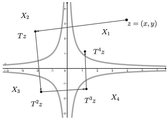
Let $(\mathbb{R}\times \mathbb{R},\parallel ·{\parallel }_2)$ be a Cartesian plane with the Euclidean norm ${\parallel ·\parallel }_2$. Let us consider the subsets $X_i\subset \mathbb{R}\times \mathbb{R}$, $i=1,2,3,4$, defined by

$$\begin{array}{c}{X}_1=\{(x,y):y\ge \frac{1}{x},0<x\}\\ X_2=\{(x,y):y\ge -\frac{1}{x},x<0\}\\ X_3=\{(x,y):y\le \frac{1}{x},x<0\}\\ X_4=\{(x,y):y\le -\frac{1}{x},x>0\}\end{array}$$

Let $T:X_1\cup X_2\cup X_3\cup X_4\to X_1\cup X_2\cup X_3\cup X_4$ be a 4–cyclic infimum summing contraction, defined by

$$T(x,y)=\left\{\begin{array}{c}(\frac{-y-1}{2},\frac{x+1}{2}),(x,y)\in X_1\\ (\frac{-y-1}{2},\frac{x-1}{2}),(x,y)\in X_2\\ (\frac{-y+1}{2},\frac{x-1}{2}),(x,y)\in X_3\\ (\frac{-y+1}{2},\frac{x+1}{2}),(x,y)\in X_4.\end{array}\right.$$

The points $(1,1)\in X_1$, $(-1,1)\in X_2$, $(-1,-1)\in X_3$ and $(1,-1)\in X_4$ are the unique fixed points for the map $T^4$ in $X_1$, respectively (Figure 8).

Figure 8. Example 1.

It is easy to see that $(1,1)\in X_1$, $(-1,1)\in X_2$, $(-1,-1)\in X_3$ and $(1,-1)\in X_4$.

Let $(x,y)\in X_1$; then, $T(x,y)=(\frac{-y-1}{2},\frac{x+1}{2})$. From $y\ge \frac{1}{x}$ and $0<x$, it follows that $x\ge -\frac{1}{-y}$ and $-y<0$, i.e., $(-y,x)\in X_2$. From the convexity of the set $X_2$ and $(-1,1)\in X_2$, it follows that $\frac{(-y,x)+(-1,1)}{2}=(\frac{-y-1}{2},\frac{x+1}{2})=T(x,y)\in X_2$, i.e., $T{X}_1\subseteq X_2$. Using similar arguments, we can prove that $T{X}_2\subseteq X_3$, $T{X}_3\subseteq X_4$ and $T{X}_4\subseteq X_1$.

It is easy to check that $T(1,1)=(-1,1)$, $T(-1,1)=(-1,-1)$, $T(-1,-1)=(1,-1)$, $T(1,-1)=(1,1)$ and $T^4(1,1)=(1,1)$, $T^4(-1,1)=(-1,1)$, $T^4(-1,-1)=(-1,-1)$, $T^4(1,-1)=(1,-1)$.

Now, we calculate $D(X_1,X_2,X_3,X_4)$.

Let $a_1=(x_1,y_1)\in X_1$, $a_2=(x_2,y_2)\in X_2$, $a_3=(x_3,y_3)\in X_3$, $a_4=(x_4,y_4)\in X_4$. Then,

$$\begin{array}{ccc}S\left({\left\{a_i\right\}}_{i=1}^4\right)\hfill & =\hfill & \parallel a_1-a_2{\parallel }_2+\parallel a_2-a_3{\parallel }_2+\parallel a_3-a_4{\parallel }_2+{\parallel a_4-a_1\parallel }_2\hfill \\ & \ge \hfill & \parallel a_1-a_2{\parallel }_{\infty }+\parallel a_2-a_3{\parallel }_{\infty }+\parallel a_3-a_4{\parallel }_{\infty }+{\parallel a_4-a_1\parallel }_{\infty }\hfill \\ & \ge \hfill & |x_1-x_2|+|y_2-y_3|+|x_3-x_4|+|y_4-y_1|.\hfill \end{array}$$

Using consecutively the inequalities $x_1>0$; $x_2<0$, $y_2>0$; $y_3<0$, $x_3<0$; $x_4>0$, $y_4<0$; $y_1>0$ and the inequality $\left|y\right|\ge |\frac{1}{x}|$ for any $(x,y)\in X_1\cup X_2\cup X_3\cup X_4$ we can write the chain of inequalities

$$\begin{array}{ccc}S\left({\left\{a_i\right\}}_{i=1}^4\right)\hfill & \ge \hfill & |x_1-x_2|+|y_2-y_3|+|x_3-x_4|+|y_4-y_1|\hfill \\ & =\hfill & |x_1|+|x_2|+|y_2|+|y_3|+|x_3|+|x_4|+|y_4|+|y_1|\hfill \\ & \ge \hfill & |x_1|+|x_2|+|\frac{1}{x_2}|+|\frac{1}{x_3}|+|x_3|+|x_4|+|\frac{1}{x_4}|+|\frac{1}{x_1}|\hfill \\ & =\hfill & \left(|x_1|+|\frac{1}{x_1}|\right)+\left(|x_2|+|\frac{1}{x_2}|\right)+\left(|x_3|+|\frac{1}{x_3}|\right)+\left(|x_4|+|\frac{1}{x_4}|\right)\ge 2,\hfill \end{array}$$

where, for the last inequality, we use the well-known one $\left|a\right|+\left|\frac{1}{a}\right|\ge 2$.

Consequently, $D(X_1,X_2,X_3,X_4)\ge 8$. There holds $S\left(\right(1,1),(-1,1),(-1,-1),(1,-1\left)\right)=8$, and thus $D(X_1,X_2,X_3,X_4)=8$.

It remains to be proven that T is a 4–cyclic infimum summing contraction, i.e., it satisfies (2).

Let $a_1=(x_1,y_1)\in X_1$ and $a_2=(x_2,y_2)\in X_2$, then

$$\begin{array}{ccc}\parallel T{a}_1-T{a}_2{\parallel }_2\hfill & =\hfill & {∥\left({\displaystyle \frac{-y_1-1}{2},\frac{x_1+1}{2}}\right)-\left({\displaystyle \frac{-y_2-1}{2},\frac{x_2-1}{2}}\right)∥}_2\hfill \\ & =\hfill & {\displaystyle \frac{\parallel (-y_1,x_1)+(-1,1)-(-y_2,x_2)-(-1,-1){\parallel }_2}{2}}\hfill \\ & \le \hfill & {\displaystyle \frac{\parallel (-y_1,x_1)-(-y_2,x_2){\parallel }_2}{2}+\frac{{\parallel (-1,1)-(-1,-1)\parallel }_2}{2}}\hfill \\ & =\hfill & {\displaystyle \frac{1}{2}\sqrt{{(y_2-y_1)}^2+{(x_1-x_2)}^2}+\frac{1}{2}.2}\hfill \\ & =\hfill & {\displaystyle \frac{1}{2}{\parallel (x_1,y_1)-(x_2,y_2)\parallel }_2+\frac{1}{2}(\frac{1}{4}D(X_1,X_2,X_3,X_4))}\hfill \\ & =\hfill & {\displaystyle \frac{1}{2}{\parallel a_1-a_2\parallel }_2+(1-\frac{1}{2})(\frac{1}{4}D(X_1,X_2,X_3,X_4)),}\hfill \end{array}$$

i.e.,

$$\parallel T{a}_1-T{a}_2{\parallel }_2\le \frac{1}{2}{\parallel a_1-a_2\parallel }_2+\left(1-\frac{1}{2}\right)\frac{D(X_1,X_2,X_3,X_4)}{4}.$$

(54)

We can prove in a similar fashion that inequality (54) holds for each $a_1\in X_i$ and $a_2\in X_{i+1}$, where $i=2,3$ and $a_1\in X_4$ and $a_2\in X_1$. Thus, for each $a_i,b_i\in X_i$, $i=1,2,3,4$, the inequalities

$$\left|\begin{array}{ccc}\hfill \parallel T{a}_1-T{b}_2{\parallel }_2& \le & \frac{1}{2}{\parallel a_1-b_2\parallel }_2+(1-\frac{1}{2})\frac{D(X_1,X_2,X_3,X_4)}{4}\hfill \\ \hfill \parallel T{a}_2-T{b}_3{\parallel }_2& \le & \frac{1}{2}{\parallel a_2-b_3\parallel }_2+(1-\frac{1}{2})\frac{D(X_1,X_2,X_3,X_4)}{4}\hfill \\ \hfill \parallel T{a}_3-T{b}_4{\parallel }_2& \le & \frac{1}{2}{\parallel a_3-b_4\parallel }_2+(1-\frac{1}{2})\frac{D(X_1,X_2,X_3,X_4)}{4}\hfill \\ \hfill \parallel T{a}_4-T{b}_1{\parallel }_2& \le & \frac{1}{2}{\parallel a_4-b_1\parallel }_2+(1-\frac{1}{2})\frac{D(X_1,X_2,X_3,X_4)}{4}\hfill \end{array}\right.$$

hold, and after summing them, we can obtain

$$\begin{array}{ccc}S\left({\left\{T{a}_i\right\}}_{i=1}^4\},{\left\{T{b}_i\right\}}_{i=1}^4\}\right)\hfill & =\hfill & {\displaystyle \parallel T{a}_4-T{b}_1{\parallel }_2+\sum _{i=1}^2{\parallel T{a}_i-T{b}_{i+1}\parallel }_2}\hfill \\ \hfill & \le \hfill & \frac{1}{2}\left({\displaystyle \parallel a_4-b_1{\parallel }_2+\sum _{i=1}^2{\parallel a_i-b_{i+1}\parallel }_2}\right)+(1-\frac{1}{2})D.\hfill \end{array}$$

(55)

Consequently, T satisfies (2) with $\lambda =\frac{1}{2}$ and $(1,1)$, $(-1,1)$, $(-1,-1)$, $(1,-1)$ are the generalized best proximity points of T in $X_1,X_2,X_3,X_4$.

This example could not be handled with the known techniques to obtain best proximity points for p–cyclic maps or even p–cyclic summing maps. Indeed if there is $x\in X_1$, which is a best proximity point of T in $X_1$, then $\parallel x-Tx\parallel =\mathrm{dist}(X_1,X_2)=0$. Actually, there are no $x_i\in X_i$, $i=1,2$, so that $\parallel x_i-x_{i+1}\parallel =\mathrm{dist}(X_i,X_{i+1})$ in the considered example.

From the definition of the sets, it follows that $\mathrm{dist}(X_i,X_{i+1})=0$ and there are no $x_i\in X_i$, satisfying $\parallel x_i-x_{i+1}\parallel =\mathrm{dist}(X_i,X_{i+1})=0$. We can alter this example by considering the a square S with vertexes $A_1=(6,0)$, $A_2=(0,6)$, $A_3=(-6,0)$ and $A_4=(0,-6)$ and replacing the sets $X_i$ with the sets $Y_i=X_i\cap S$ (Figure 9). Then, $\mathrm{dist}(Y_i,Y_{i+1})=r>0$ for $i=1,2,3,4$. If we consider the map T, defined on the sets $Y_i$, $i=1,2,3,4$, this will satisfy the conditions of (2) as far as $T\left(Y_i\right)\subset Y_{i+1}$. If $x_1\in Y_1$ is a best proximity point of T in $Y_1$, then $x_2=T{x}_1\in Y_2$ and $\parallel x_1-T{x}_1\parallel =\mathrm{dist}(Y_1,Y_2)=r$ (Figure 9). Furthermore if $y_2\in Y_2$ is a best proximity point of T in $Y_2$, then $y_3=T{x}_2\in Y_3$ and $\parallel y_2-T{y}_2\parallel =\mathrm{dist}(Y_2,Y_3)=r$ (Figure 9). All known results about best proximity points ensure that $x_2=y_2$, which is not the case in the considered example.

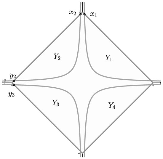
Figure 9. Example 1 with the sets $Y_i=S\cap X_i$.

7. Discussion

We presented a generalization of the notion of best proximity points [2,34,36] and illustrated that the new notion of a generalized best proximity point and p–cyclic infimum summing maps is different from the known classical ones. It will be interesting to see whether generalizations of Kannan, Chatterjea, Hardy–Roger or Meir–Keeler types of maps can be obtained for infimum-summing maps.

As we mentioned in the Section 1, the idea to consider the infimum sum focused on the widely investigated TSP in the case where a convex hulls of the cluster are considered. There are a lot of results in this field and applications in different fields, such as computer wiring [44], wallpaper cutting [45], hole punching [46], dartboard design [47], crystallography [48], and vehicle routing [44]. The most recent applications are finding the best route for the inspection of transmission infrastructure using Unmanned Aerial Vehicles (UAV) [49,50]. When the TSP is considered for UAVs, naturally, the classical discrete optimization techniques can be altered to continuous ones. It will be interesting to see whether it is possible to apply the main results to solve some of the TSP set in the continuous setting.

References

- Kirk, W.; Srinivasan, P.; Veeramani, P. Fixed Points for Mappings Satisfying Cyclical Contractive Conditions. Fixed Point Theory 2003, 4, 79–189. Available online: http://www.math.ubbcluj.ro/~nodeacj/download.php?f=031Kirk.pdf (accessed on 23 June 2023).
- Eldred, A.; Veeramani, P. Existence and convergence of best proximity points. J. Math. Anal. Appl. 2006, 323, 1001–1006. [Google Scholar] [CrossRef]
- Ali, B.; Khan, A.A.; De la Sen, M. Optimum Solutions of Systems of Differential Equations via Best Proximity Points in b-Metric Spaces. Mathematics 2023, 11, 574. [Google Scholar] [CrossRef]
- Aloqaily, A.; Souayah, N.; Matawie, K.; Mlaiki, N.; Shatanawi, W. A New Best Proximity Point Results in Partial Metric Spaces Endowed with a Graph. Symmetry 2023, 15, 611. [Google Scholar] [CrossRef]
- Felhi, A. Best Proximity Results for Multi-Valued α-F–Proximal Contractive Mappings. Thai J. Math. 2023, 21, 139–152. [Google Scholar]
- Lateef, D. Best proximity points in f-metric spaces with applications. Demonstr. Math. 2023, 56, 20220191. [Google Scholar] [CrossRef]
- Patel, U.D.; Todorcevic, V.; Radojevic, S.; Radenović, S. Best Proximity Point for Γ-F–Fuzzy Proximal Contraction. Axioms 2023, 12, 165. [Google Scholar] [CrossRef]
- Sultana, A. Best proximity points of set-valued generalized contractions. Fixed Point Theory 2023, 24, 383–392. [Google Scholar] [CrossRef]
- Usurelu, G.I.; Bejenaru, A.; Postolache, M. Reaching Takahashi-type nonexpansive operators via modular structures with application to best proximity point. Adv. Oper. Theory 2023, 8, 22. [Google Scholar] [CrossRef]
- Baria, C.; Suzuki, T.; Vetroa, C. Best proximity points for cyclic Meir–Keeler contractions. Nonlinear Anal. Theory Methods Appl. 2008, 69, 3790–3794. [Google Scholar] [CrossRef]
- Petric, M. Best proximity point theorems for weak cyclic Kannan contractions. Filomat 2011, 25, 145–154. [Google Scholar] [CrossRef]
- Suzuki, T.; Kikkawa, M.; Vetro, C. The existence of best proximity points in metric spaces with the property UC. Nonlinear Anal. Theory Methods Appl. 2009, 71, 2918–2926. [Google Scholar] [CrossRef]
- Sintunavarat, W.; Kumam, P. Coupled best proximity point theorem in metric spaces. Fixed Point Theory Appl. 2012, 2012, 93. [Google Scholar] [CrossRef]
- Zhelinski, V.; Zlatanov, B. On the UC and UC* properties and the existence of best proximity points in metric spaces. arXiv 2023, arXiv:2303.05850. [Google Scholar]
- Ben-Arieh, D.; Gutin, G.; Penn, M.; Yeo, A.; Zverovitch, A. Transformations of generalized ATSP into ATSP. Oper. Res. Lett. 2003, 31, 357–365. [Google Scholar] [CrossRef]
- Fischetti, M.; González, J.J.S.; Toth, P. A Branch-and-Cut algorithm for the symmetric generalized traveling salesman problem. Oper. Res. 1997, 45, 378–394. [Google Scholar] [CrossRef]
- Gutin, G.; Karapetyan, D. A Memetic Algorithm for the Generalized Traveling Salesman Problem. Nat. Comput. 2010, 9, 47–60. [Google Scholar] [CrossRef]
- Noon, C.E. The Generalized Traveling Salesman Problem. Ph.D. Thesis, University of Michigan Library, Ann Arbor, MI, USA, 1992. Available online: https://hdl.handle.net/2027.42/161841 (accessed on 23 June 2023).
- Noon, C.E.; Bean, J.C. An efficient transformation of the generalized traveling salesman problem. INFOR Inf. Syst. Oper. Res. 1993, 31, 39–44. [Google Scholar] [CrossRef]
- Pintea, C.-M.; Pop, P.C.; Chira, C. The generalized traveling salesman problem solved with ant algorithms. Complex Adapt. Syst. Model. 2017, 5, 8. [Google Scholar] [CrossRef]
- Manyam, S.G.; Rathinam, S.; Darbha, S.; Casbeer, D.; Cao, Y.; Chandler, P. GPS Denied UAV Routing with Communication Constraints. J. Intell. Robot. Syst. 2016, 84, 691–703. [Google Scholar] [CrossRef]
- Manyam, S.G.; Rathinam, S. On Tightly Bounding the Dubins Traveling Salesman’s Optimum. J. Dyn. Syst. Meas. Control Trans. ASME 2018, 140, 071013. [Google Scholar] [CrossRef]
- Manyam, S.G.; Rathinam, S.; Casbeer, D.; Garcia, E. Tightly Bounding the Shortest Dubins Paths Through a Sequence of Points. J. Intell. Robot. Syst. 2017, 88, 495–511. [Google Scholar] [CrossRef]
- Silberholz, J.; Golden, B. The Generalized Traveling Salesman Problem: A new Genetic Algorithm approach. In Extending the Horizons: Advances in Computing, Optimization, and Decision Technologies; Springer: Berlin/Heidelberg, Germany, 2007; Volume 37, pp. 165–181. [Google Scholar] [CrossRef]
- Snyder, L.V.; Daskin, M.S. A random-key genetic algorithm for the generalized traveling salesman problem. Eur. J. Oper. Res. 2006, 174, 38–53. [Google Scholar] [CrossRef]
- Laporte, G. The traveling salesman problem: An overview of exact and approximate algorithms. Eur. J. Oper. Res. 1992, 59, 231–247. [Google Scholar] [CrossRef]
- Lawler, E.L.; Lenstra, J.K.; Rinnooy Kan, A.H.G.; Shmoys, D.B. The Traveling Salesman Problem: A Guided Tour of Combinatorial Optimization; A Wiley-Interscience Publication: Chichester, UK; New York, NY, USA; Brisbane, Australia; Toronto, ON, Canada; Singapore, 1985. [Google Scholar]
- Dimitrijević, V.; Šarić, Z. An Efficient Transformation of the Generalized Traveling Salesman Problem into the Traveling Salesman Problem on Digraphs. Inf. Sci. 1997, 102, 105–110. [Google Scholar] [CrossRef]
- Dror, M.; Langevin, A. A generalized traveling salesman problem approach to the directed clustered rural postman problem. Transp. Sci. 1997, 31, 187–192. [Google Scholar] [CrossRef]
- Karpagam, S.; Agrawal, S. Existence of Best Proximity Points of P–Cyclic Contractions. Fixed Point Theory 2012, 13, 99–105. Available online: http://www.math.ubbcluj.ro/~nodeacj/download.php?f=121Karpagam-final.pdf (accessed on 23 June 2023).
- Li, Y.; Li, S.; Zhang, Y.; Zhang, W.; Lu, H. Dynamic Route Planning for a USV-UAV Multi-Robot System in the Rendezvous Task with Obstacles. J. Intell. Robot. Syst. Theory Appl. 2023, 107, 52. [Google Scholar] [CrossRef]
- Mignardi, S.; Buratti, C. Modelling UAV-based IoT Clustered Networks For Reduced Capability UEs. IEEE Internet Things J. 2023, in press. [CrossRef]
- Zhu, Y.; Wang, S. Flying Path Optimization of Rechargeable UAV for Data Collection in Wireless Sensor Networks. IEEE Sens. Lett. 2023, 7, 7500104. [Google Scholar] [CrossRef]
- Karpagam, S.; Agrawal, S. Best proximity point theorems for p–cyclic Meir-Keeler contractions. Fixed Point Theory Appl. 2009, 2009, 197308. [Google Scholar] [CrossRef]
- Karpagam, S.; Zlatanov, B. Best proximity points of p–cyclic orbital Meir–Keeler contraction maps. Nonlinear Anal. Model. Control. 2016, 21, 790–806. [Google Scholar] [CrossRef]
- Petric, M.; Zlatanov, B. Best proximity points and fixed points for p–summing maps. Fixed Point Theory Appl. 2012, 2012, 86. [Google Scholar] [CrossRef]
- Petric, M.; Zlatanov, B. Best Proximity Points for p–Cyclic Summing Iterated Contractions. FILOMAT 2018, 32, 3275–3287. [Google Scholar] [CrossRef]
- Zlatanov, B. Best Proximity Points for p-Summing Cyclic Orbital Meir-Keeler Contractions. Nonlinear Anal. Model. Control 2015, 20, 528–544. [Google Scholar] [CrossRef]
- Karpagam, S.; Zlatanov, B. A note on best proximity points for p–summing cyclic orbital Meir-Keeler contractions. Int. J. Pure Appl. Math. 2016, 107, 225–243. [Google Scholar] [CrossRef]
- Fabian, M.; Habala, P.; Hájek, P.; Montesinos, V.; Zizler, V. Banach Space Theory; Springer: New York, NY, USA, 2001. [Google Scholar]
- Deville, R.; Godefroy, G.; Zizler, V. Smothness and Renormings in Banach Spaces; Longman Scientific Technical: Harlow, UK; John Wiley Sons, Inc.: New York, NY, USA, 1993. [Google Scholar]
- Fabian, M.; Habala, P.; Hájek, P.; Montesinos, V.; Pelant, J.; Zizler, V. Functional Analysis and Infinite–Dimensional Geometry—The Basis for Linear and Nonlinear Analysis; Springer: New York, NY, USA; Dordrecht, The Netherlands; Berlin/Heidelberg, Germany; London, UK, 2011. [Google Scholar] [CrossRef]
- O’Searcóid, M. Metric Spaces; Springer: Berlin/Heidelberg, Germany, 2006. [Google Scholar] [CrossRef]
- Lenstra, J.K.; Rinnooy Kan, A.H.G. Some Simple Applications of the Travelling Salesman Problem. Oper. Res. Q. 1975, 26, 717–733. [Google Scholar] [CrossRef]
- Garfinkel, R.S. Minimizing wallpaper waste, Part I: A class of traveling salesman problems. Oper. Res. 1977, 25, 741–751. [Google Scholar] [CrossRef]
- Reinelt, G. Fast Heuristics for Large Geometric Traveling Salesman Problems; Report No. 185; Institut fiir Mathematik, Universit it Augsburg: Augsburg, Germany, 1989. [Google Scholar]
- Eiselt, H.A.; Laporte, G. A combinatorial optimization problem arising in dartboard design. J. Oper. Res. Soc. 1991, 42, 113–118. [Google Scholar] [CrossRef]
- Bland, R.G.; Shallcross, D.F. Large traveling salesman problems arising experiments in X-ray crystallography: A preliminary report on computation. Oper. Res. Lett. 1989, 8, 125–128. [Google Scholar] [CrossRef]
- Papaioannou, S.; Kolios, P.; Theocharides, T.; Panayiotou, C.G.; Polycarpou, M.M. UAV-based Receding Horizon Control for 3D Inspection Planning. In Proceedings of the 2022 International Conference on Unmanned Aircraft Systems (ICUAS), Dubrovnik, Croatia, 21–24 June 2022. [Google Scholar] [CrossRef]
- Nekovar, F.; Faigl, J.; Saska, M. Multi-tour Set Traveling Salesman Problem in Planning Power Transmission Line Inspection. IEEE Robot. Autom. Lett. 2021, 6, 6196–6203. [Google Scholar] [CrossRef]
Disclaimer/Publisher’s Note: The statements, opinions and data contained in all publications are solely those of the individual author(s) and contributor(s) and not of MDPI and/or the editor(s). MDPI and/or the editor(s) disclaim responsibility for any injury to people or property resulting from any ideas, methods, instructions or products referred to in the content. |
© 2023 by the authors. Licensee MDPI, Basel, Switzerland. This article is an open access article distributed under the terms and conditions of the Creative Commons Attribution (CC BY) license (https://creativecommons.org/licenses/by/4.0/).