Statistical Analysis and Applications of Adaptive Progressively Type-II Hybrid Poisson–Exponential Censored Data

Abstract

A new two-parameter extended exponential lifetime distribution with an increasing failure rate called the Poisson–exponential (PE) model was explored. In the reliability experiments, an adaptive progressively Type-II hybrid censoring strategy is presented to improve the statistical analysis efficiency and reduce the entire test duration on a life-testing experiment. To benefit from this mechanism, this paper sought to infer the unknown parameters, as well as the reliability and failure rate function of the PE distribution using both the likelihood and product of spacings estimation procedures as a conventional view. For each unknown parameter, from both classical approaches, an approximate confidence interval based on Fisher’s information was also created. Additionally, in the Bayesian paradigm, the given classical approaches were extended to Bayes’ continuous theorem to develop the Bayes (or credible interval) estimates of the same unknown quantities. Employing the squared error loss, the Bayesian inference was developed based on independent gamma assumptions. Because of the complex nature of the posterior density, the Markov chain with the Monte Carlo methodology was used to obtain data from the whole conditional distributions and, therefore, evaluate the acquired Bayes point/interval estimates. Via extensive numerical comparisons, the performance of the estimates provided was evaluated with respect to various criteria. Among different competing progressive mechanisms, using four optimality criteria, the best censoring was suggested. Two real chemical engineering datasets were also analyzed to highlight the applicability of the acquired point and interval estimators in an actual practical scenario.

1. Introduction

In reliability experiments, the exponential lifetime model gives a straightforward, elegant, and closed-form result for many issues. It does not, however, give a suitable parametric fit for several actual situations in which the underlying hazard rates are nonconstant, resulting in monotone forms. As a result, in probability theory, new modifications of the exponential distribution have been created to describe specific real-life data. A new two-parameter statistical model with an increasing failure rate as a possible extension to the well-known exponential model called the Poisson–exponential (PE) distribution was introduced by Cancho et al. [1]. They also studied several characteristics of the PE distribution. However, a lifetime random variable of a test subject (or item) (say X) is said to have a two-parameter PE distribution, denoted by $\mathrm{PE}(\mathsf{\Omega })$, where $\mathsf{\Omega }={(\mu ,\gamma )}^{\mathsf{T}}$ is the parameter vector, with shape parameter $\gamma >0$ and scale parameter $\mu >0$, if its probability density function (PDF), $f(·)$, and the cumulative distribution function (CDF), $F(·)$, are given (for $x>0$) by

$$f(x;\mathsf{\Omega })=\frac{\gamma \mu exp(-\mu x-\gamma e^{-\mu x})}{1-e^{-\gamma }},$$

(1)

and

$$F(x;\mathsf{\Omega })=1-\left[\frac{1-exp(-\gamma e^{-\mu x})}{1-e^{-\gamma }}\right],$$

(2)

respectively.

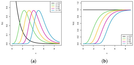
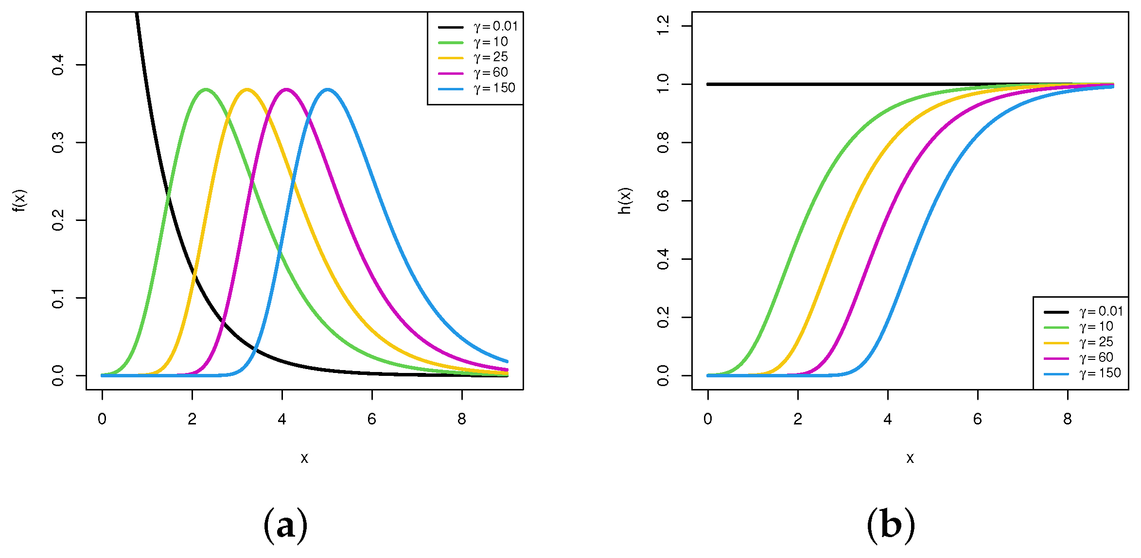
One can see that the PE distribution has reverted to an exponential distribution with parameter $\mu$ when $\gamma \to 0$. Taking $\mu =1$, Figure 1a shows that the PE density (1) is decreasing for $0<\gamma <1$ and unimodal for $\gamma ⩾1$. On the other hand, two time characteristics of the PE distribution can be considered as unknown parameters, namely: reliability time function (RF), $R(·)$, and hazard rate (or failure) function (HRF), $h(·)$, at distinct time t, which are given (for $t>0$) by

$$R(t;\mathsf{\Omega })=\frac{1-exp(-\gamma e^{-\mu t})}{1-e^{-\gamma }},t>0,$$

(3)

and

$$h(t;\mathsf{\Omega })=\frac{\gamma \mu exp(-\mu t-\gamma e^{-\mu t})}{1-exp(-\gamma e^{-\mu t})},$$

(4)

respectively. Figure 1b indicates that the PE failure rate (4), for the same fixed value of $\mu$, is increasing.

From an engineering point of view, the concept of an increasing failure rate is very attractive because it is often associated with a mathematical depiction of failure. Independently, using a complete sample, Louzada-Neto et al. [2], Singh et al. [3], and Rodrigues et al. [4] derived different estimators of the PE parameters. In the reliability context, due to the flexibility and adaptability of the PE model for modeling time data points, different studies using the PE model have been achieved; for example, Kumar et al. [5] discussed the reliability estimation for the PE model using progressive Type-II censoring (T2PC) with binomials; Gitahi et al. [6] considered the expectation–maximization algorithm to estimate the PE parameters in the presence of T2PC data; Arabi Belaghi et al. [7] discussed the PE parameters using Type-II censoring; Mohammadi Monfared [8] explored both the estimation and prediction problems of the PE model using Type-I hybrid censoring, among others.

Adaptive progressively Type-II hybrid censoring (AT2PHC), introduced by Ng et al. [9], aims to handle the main problem in progressive Type-II censoring, that the length of the effective censored sample size is too small, and then, the extrapolated results become insignificant. At time zero, $T=0$, this mechanism starts with n units being put to a test; r is a prefixed number of failed subjects, and $\mathbf{R}=(R_1,\dots ,R_r)$ is a prefixed progressive censoring. Once the first failure $X_{1:r:n}$ is recorded, the surviving units $R_1$ of $n-1$ are randomly removed and taken out of the test. Next, as soon as the second failure $X_{2:r:n}$ is recorded, the surviving units $R_2$ of $n-2-R_1$ are removed, and so on. If $X_{r:r:r}<T$, the experiment ends at $X_{r:r:r}$ with the same removals $\mathbf{R}$ determined beforehand. Otherwise, if $X_{r:r:r}>T$, we stop removing any remaining element, i.e., $R_j=0$ for $j=m+1,\dots ,r-1$, where m is the number of failure times occurring before T. Then, end the test at T, and remove the remaining $R_r=n-r-{\sum }_{j=1}^m{R}_j$ items.

This modification permits running over T with some $R_j,j=1,\dots ,r-1$ members potentially altered throughout the test and ensures that the test is terminated with an efficient number of r, and the overall test time will not be isolated from the threshold point T. Suppose that $x_{1:r:n}<\cdots <x_{m:r:n}<T<x_{m+1:r:n}<\dots x_{r:r:n}$ is an AT2PHC sample from a lifetime population with the PDF (say $f(·)$) and CDF (say $F(·)$), then the likelihood function (LF) is

$$\mathcal{L}(\mathsf{\Omega })=k\prod _{j=1}^{r}f(x_{j:r:n};\mathsf{\Omega })\prod _{j=1}^m{\left[R(x_{j:r:n};\mathsf{\Omega })\right]}^{R_j}{\left[R(x_{r:r:n};\mathsf{\Omega })\right]}^{R_r},$$

(5)

where k is a constant.

Using the AT2PHC strategy, several works have been performed in the literature; for example, see Hemmati and Khorram [10], Liu and Gui [11], Kohansal and Bakouch [12], Elshahhat and Nassar [13], Du and Gui [14], Ateya et al. [15], Alotaibi et al. [16], Nassar et al. [17], Elshahhat and Nassar [18], and the references cited therein.

In past years, researchers have often used the product of spacings approach as a favorable alternative to the basic likelihood method. Cheng and Amin [19] and Ranneby [20] independently proposed the maximum product of spacings (MPS) approach and stated that it maintains the entirety of the features of the likelihood estimates, such as efficiency, consistency, and sufficiency. Similar to the LF approach, the MPS approach provides the invariance characteristic in the suggested estimates; see Anatolyev and Kosenok [21]. Directly, via maximizing the product of the discrepancies between the distribution function values at nearby ascending order points, the MPS estimator (MPSE) is presented. However, following Ng et al. [22], the product of spacings function (SF) of the AT2PHC plan can be expressed as

$$\mathcal{P}(\mathsf{\Omega })=\prod _{j=1}^{r+1}{S}_j\prod _{j=1}^m{\left[R(x_{j:r:n};\mathsf{\Omega })\right]}^{R_j}{\left[R(x_{r:r:n};\mathsf{\Omega })\right]}^{R_r},$$

(6)

where $S_j=F(x_{j:r:n};\mathsf{\Omega })-F(x_{j-1:r:n};\mathsf{\Omega })$, $F(x_{0:r:n};\mathsf{\Omega })\equiv 0$, and $F(x_{r+1:r:n};\mathsf{\Omega })\equiv 1$.

Several works have considered the SF besides (or instead of) the LF; see, for example, Singh et al. [23], Basu et al. [24], Yalçınkaya et al. [25], Jeon et al. [26], Nassar et al. [27], and Dey and Elshahhat [28], among others.

In the literature, we have not come across any work that discusses the statistical characteristics of the proposed distribution and/or estimates its parameters under AT2PHC sampling. To the best of our knowledge, when an adaptive progressively Type-II hybrid censored dataset is collected, this work is unique in that it is the first study to compare two Bayesian and classical (using LF and SF approaches) methods of the PE’s parameters or its reliability characteristics. We may motivate this work by pointing out: (i) the importance of AT2PHC in improving parameter estimation efficiency by striving to avoid small observed sample sizes; (ii) the PE distribution’s adaptability in modeling many kinds of datasets with an increasing failure rate shape.

To achieve this goal, this study has five objectives:

• Estimate the parameters ($\mu ,\gamma$), RF $R(t)$, and HRF $h(t)$ functions of the PE distribution using the LF and SF methods using an adaptive progressively Type-II hybrid censoring. Approximate confidence interval (ACI) estimates of $\mu$, $\gamma$, $R(t)$, and $h(t)$, based on both frequentist approaches, were also obtained.
• Drive the Bayesian estimates via the LF- and SF-based estimation of the same objective parameters under the squared error loss (SEL) function from independent gamma priors. These estimates cannot be computed mathematically, so Monte Carlo Markov chain (MCMC) techniques were utilized.
• Determine the best progressive design, based on four different optimality criteria, that conveys a significant quantity of information about the model parameter(s) of interest.
• Evaluate the suggested approaches’ effectiveness in terms of the root-mean-squared error, relative absolute bias, average interval length, and coverage probability through several numerical comparisons.
• Two applications based on real-world chemical engineering datasets illustrate the PE distribution’s ability to fit different data types and adapt the proposed approaches to actual practical situations.

The rest of the paper is organized as follows: The frequentist and Bayes estimates are derived in Section 2 and Section 3, respectively. Section 4 gives the Monte Carlo outputs. Section 5 reports various criteria for obtaining the best progressive plan. Section 6 investigates two real applications. Ultimately, Section 7 concludes the paper.

2. Frequentist Estimators

This section aims to derive both point and interval estimates of $\mu$, $\gamma$, $R(t)$, and $h(t)$ of the PE model from AT2PHC via the LF and SF techniques.

2.1. Likelihood Inference

Let $\mathbf{x}=\{(x_{1:r:n},R_1),\dots ,(x_{m:r:n},R_m),T,(x_{m+1:r:n},0),\dots ,(x_{r-1:r:n},0),(x_{r:r:n},R_r)\}$ be the observed AT2PHC data with size r created from the PE distribution with density (1) and distribution (2) functions. Then, the LF for these data, where the constant term is ignored and $x_i=x_{i:r:n}$ is used for simplicity, becomes

$$\mathcal{L}(\mathsf{\Omega }|\mathbf{x})\propto {(1-e^{-\gamma })}^{-n}{(\gamma \mu )}^{r}exp\left(-\left[\mu r\overline{x}+\Psi (\mu ,\gamma )+\gamma {\sum }_{j=1}^r{e}^{-\mu x_j}\right]\right),$$

(7)

where $\Psi (\mu ,\gamma )=-{\displaystyle \sum _{j=1}^m}{R}_{j}log\left[1-exp\left(-\gamma e^{-\mu x_j}\right)\right]-R_{r}log\left[1-exp\left(-\gamma e^{-\mu x_r}\right)\right].$

As a result, from (7), the log-likelihood function ($l(·)\propto log\mathcal{L}(·)$) becomes

$$\begin{array}{c}\hfill l(\mathsf{\Omega }|\mathbf{x})\propto -nlog(1-e^{-\gamma })+rlog(\gamma \mu )-\mu r\overline{x}-\Psi (\mu ,\gamma )-\gamma \sum _{j=1}^r{e}^{-\mu x_j}.\end{array}$$

(8)

The MLEs $\widehat{\mu }$ and $\widehat{\gamma }$ of $\mu$ and $\gamma$, respectively, can be easily offered by simultaneously solving the following two normal formulas:

$$\frac{\partial l}{\partial \mu }=r{\mu }^{-1}-r\overline{x}-\gamma {\sum }_{j=1}^r{x}_j{e}^{-\mu x_j}-{\Psi }_{\mu }^1(\mu ,\gamma ),$$

(9)

and

$$\frac{\partial l}{\partial \gamma }=-n{e}^{-\gamma }{(1-e^{-\gamma })}^{-1}+r{\gamma }^{-1}+{\sum }_{j=1}^r{e}^{-\mu x_j}+{\Psi }_{\gamma }^1(\mu ,\gamma ),$$

(10)

where

$$\begin{array}{cc}\hfill {\Psi }_{\mu }^1(\mu ,\gamma )& =\gamma {\sum }_{j=1}^m{R}_j{x}_{j}exp\left(-\mu x_j-\gamma e^{-\mu x_j}\right){\left(1-exp\left(-\gamma e^{-\mu x_j}\right)\right)}^{-1}\hfill \\ \hfill & +\gamma R_r{x}_{r}exp\left(-\mu x_r-\gamma e^{-\mu x_r}\right){\left(1-exp\left(-\gamma e^{-\mu x_r}\right)\right)}^{-1},\hfill \end{array}$$

and

$$\begin{array}{cc}\hfill {\Psi }_{\gamma }^1(\mu ,\gamma )& ={\sum }_{j=1}^m{R}_{j}exp\left(-\mu x_j-\gamma e^{-\mu x_j}\right){\left(1-exp\left(-\gamma e^{-\mu x_j}\right)\right)}^{-1}\hfill \\ \hfill & +R_{r}exp\left(-\mu x_r-\gamma e^{-\mu x_r}\right){\left(1-exp\left(-\gamma e^{-\mu x_r}\right)\right)}^{-1}.\hfill \end{array}$$

It is obvious, from (9) and (10), that the MLEs $\widehat{\mu }$ and $\widehat{\gamma }$ of $\mu$ and $\gamma$, respectively, cannot be formulated in explicit forms. Therefore, for given T, r, and $\mathbf{R}$, we suggest in this case the Newton–Raphson method to evaluate the MLEs $\widehat{\mu }$ and $\widehat{\gamma }$. To achieve this goal, the ”$\mathsf{maxLik}$” package, proposed by Henningsen and Toomet [29], is recommended.

Once the estimates of $\mu$ and $\gamma$ are obtained, the invariance property of $\widehat{\mu }$ and $\widehat{\gamma }$ is utilized in turn to estimate the MLEs of $R(t)$ and $h(t)$ at a specified time t as

$$\widehat{R}(t)=\frac{1-exp(-\widehat{\gamma }{e}^{-\widehat{\mu }t})}{1-e^{-\widehat{\gamma }}}\mathrm{and}\widehat{h}(t)=\frac{\widehat{\gamma }\widehat{\mu }exp(-\widehat{\mu }t-\widehat{\gamma }{e}^{-\widehat{\mu }t})}{1-exp(-\widehat{\gamma }{e}^{-\widehat{\mu }t})},$$

respectively.

Now, to get the ACI of $\mu$, $\gamma$, $R(t)$, or $h(t)$, we utilized their asymptotic properties. According to the theory of large samples, the distribution of $\widehat{\mathsf{\Omega }}$, where $\widehat{\mathsf{\Omega }}$ is the MLE of $\mathsf{\Omega }$, is a bivariate normal with mean $\mathsf{\Omega }$ and variance–covariance (VC) matrix ${\mathbf{I}}_{\mathcal{L}}^{-1}(\mathsf{\Omega })$. Due to the nonlinear form of (7), the Fisher information matrix cannot be used directly to obtain such a VC matrix. Thus, by replacing $\mu$ and $\gamma$ with their $\widehat{\mu }$ and $\widehat{\gamma }$, respectively, we can estimate ${\mathbf{I}}_{\mathcal{L}}^{-1}(\mathsf{\Omega })$ by ${\mathbf{I}}_{\mathcal{L}}^{-1}(\widehat{\mathsf{\Omega }})$ as

$${\mathbf{I}}_{\mathcal{L}}^{-1}(\widehat{\mathsf{\Omega }})={\left[\begin{array}{cc}-{\mathcal{L}}_{11}& -{\mathcal{L}}_{12}\\ -{\mathcal{L}}_{21}& -{\mathcal{L}}_{22}\end{array}\right]}_{(\mu ,\gamma )=(\widehat{\mu },\widehat{\gamma })}^{-1}=\left[\begin{array}{cc}{\widehat{\sigma }}_{11}& {\widehat{\sigma }}_{12}\\ {\widehat{\sigma }}_{21}& {\widehat{\sigma }}_{22}\end{array}\right],$$

(11)

where the elements ${\mathcal{L}}_{ij},i,j=1,2$ are obtained; see Appendix A.

Presently, the two bounds of $100(1-\pi )\%$ ACIs of $\mu$ and $\gamma$ can be obtained as

$$\widehat{\mu }\pm z_{\pi /2}\sqrt{{\widehat{\sigma }}_{11}}\mathrm{and}\widehat{\gamma }\pm z_{\pi /2}\sqrt{{\widehat{\sigma }}_{22}},$$

respectively, where ${\widehat{\sigma }}_{ii}$ for $i=1,2$ are obtained in (11) and $z_{\pi /2}$ is the upper ${(\pi /2)}^{th}$ percentile point of the standard normal distribution.

Further, to create the ACI of $R(t)$ or $h(t)$, the variance of $\widehat{R}(t)$ and $\widehat{h}(t)$ must be obtained first. Greene [30] pointed out that the delta method is one of the most-popular ways to approximate the variance of an unknown parametric function. However, the associated variance of $R(t)$ and $h(t)$ denoted by ${\widehat{\sigma }}_R$ and ${\widehat{\sigma }}_h$, respectively, can be approximated at $(\mu ,\gamma )=(\widehat{\mu },\widehat{\gamma })$ as

$${\widehat{\sigma }}_R={\mathcal{D}}_R{\mathbf{I}}_{\mathcal{L}}^{-1}(\widehat{\mathsf{\Omega }}){\mathcal{D}}_R^{\top }\mathrm{and}{\widehat{\sigma }}_h={\mathcal{D}}_h{\mathbf{I}}_{\mathcal{L}}^{-1}(\widehat{\mathsf{\Omega }}){\mathcal{D}}_h^{\top },$$

(12)

where ${\mathcal{D}}_R=\left[\frac{\partial R}{\partial \mu }\frac{\partial R}{\partial \gamma }\right]$ and ${\mathcal{D}}_h=\left[\frac{\partial h}{\partial \mu }\frac{\partial h}{\partial \gamma }\right]$ are given by

$$\begin{array}{c}\frac{\partial R}{\partial \mu }=1-\gamma e^{-\mu t}\left\{1+exp(-\gamma e^{-\mu t}){(1-exp(-\gamma e^{-\mu t}))}^{-1}\right\},\hfill \\ \frac{\partial R}{\partial \gamma }=\left[exp(-\mu t-\gamma e^{-\mu t})-(1-exp(-\gamma e^{-\mu t}))e^{-\gamma }{(1-e^{-\gamma })}^{-1}\right]{(1-e^{-\gamma })}^{-1},\hfill \\ \begin{array}{cc}\hfill \frac{\partial h}{\partial \mu }& =\gamma exp(-\mu t-\gamma e^{-\mu t}){(1-exp(-\gamma e^{-\mu t}))}^{-1}\hfill \\ \hfill & \times \left\{1+\mu t\left[\gamma e^{-\mu t}\left\{1+exp(-\gamma e^{-\mu t}){(1-exp(-\gamma e^{-\mu t}))}^{-1}\right\}-1\right]\right\},\hfill \end{array}\hfill \end{array}$$

and

$$\begin{array}{cc}\hfill \frac{\partial h}{\partial \gamma }& =\mu exp(-\mu t-\gamma e^{-\mu t}){(1-exp(-\gamma e^{-\mu t}))}^{-1}\hfill \\ \hfill & \times \left[1-\gamma e^{-\mu t}\left\{1+exp(-\gamma e^{-\mu t}){(1-exp(-\gamma e^{-\mu t}))}^{-1}\right\}\right].\hfill \end{array}$$

As a result, from (12), the two-sided ACIs of $R(t)$ and $h(t)$ at a confidence level of $100(1-\pi )\%$ are

$$\widehat{R}(t)\pm z_{\frac{\pi }{2}}\sqrt{{\widehat{\sigma }}_R},$$

and

$$\widehat{h}(t)\pm z_{\frac{\pi }{2}}\sqrt{{\widehat{\sigma }}_h},$$

respectively.

2.2. Product of Spacing Inference

Given an AT2PHC sample of size r collected from the PE population, based on (1) and (2), the SF (6) can be expressed as

$$\begin{array}{c}\hfill \mathcal{P}\left(\left.\mathsf{\Omega }\right|\mathbf{x}\right)\propto {(1-e^{-\gamma })}^{-(n+1)}{e}^{-\Psi (\mu ,\gamma )}\prod _{j=1}^r\left[exp\left(-\gamma e^{-\mu x_j}\right)-exp\left(-\gamma e^{-\mu x_{j-1}}\right)\right],\end{array}$$

(13)

where $\Psi (\mu ,\gamma )$ is defined in (7).

Equivalently, taking the natural logarithm of ($p(·)\propto log\mathcal{P}(·)$), we obtain

$$\begin{array}{c}\hfill p\left(\left.\mathsf{\Omega }\right|\mathbf{x}\right)\propto -(n+1)log(1-e^{-\gamma })-\Psi (\mu ,\gamma )+\sum _{j=1}^{r}log\left[exp\left(-\gamma e^{-\mu x_j}\right)-exp\left(-\gamma e^{-\mu x_{j-1}}\right)\right].\end{array}$$

(14)

Differentiating (14) (partially) with respect to $\mu$ and $\gamma$, the MPSEs $\check{\mu }$ and $\check{\gamma }$ of $\mu$ and $\gamma$ can be offered by solving the following nonlinear equations:

$$\begin{array}{cc}\hfill \frac{\partial p}{\partial \mu }=-{\Psi }_{\mu }^1(\mu ,\gamma )+\gamma \sum _{j=1}^r& \{\left\{x_{j}exp\left(-\mu x_j-\gamma e^{-\mu x_j}\right)-x_{j-1}exp\left(-\mu x_{j-1}-\gamma e^{-\mu x_{j-1}}\right)\right\}\hfill \\ \hfill & \times {\left[exp\left(-\gamma e^{-\mu x_j}\right)-exp\left(-\gamma e^{-\mu x_{j-1}}\right)\right]}^{-1}\},\hfill \end{array}$$

(15)

and

$$\begin{array}{cc}\hfill \frac{\partial p}{\partial \gamma }=-\frac{(n+1)e^{-\gamma }}{(1-e^{-\gamma })}-{\Psi }_{\gamma }^1(\mu ,\gamma )+\sum _{j=1}^r& \{\left\{exp\left(-\mu x_{j-1}-\gamma e^{-\mu x_{j-1}}\right)-exp\left(-\mu x_j-\gamma e^{-\mu x_j}\right)\right\}\hfill \\ \hfill & \times {\left[exp\left(-\gamma e^{-\mu x_j}\right)-exp\left(-\gamma e^{-\mu x_{j-1}}\right)\right]}^{-1}\},\hfill \end{array}$$

(16)

respectively.

Since the expressions of $\check{\mu }$ and $\check{\gamma }$ as in (15) and (15), respectively, cannot be solved mathematically, so the Newton–Raphson technique via the “$\mathsf{maxLik}$” package, proposed by Henningsen and Toomet [29], is suggested to obtain $\check{\mu }$ and $\check{\gamma }$. One of the best characteristics of the MPSE, similar to the MLE, is that it has consistent, asymptotic, and invariance characteristics; see Cheng and Traylor [31]. Thus, the MPSEs $\check{R}(t)$ and $\check{h}(t)$ of $R(t)$ and $h(t)$ can be acquired, respectively, as

$$\check{R}(t)=\frac{1-exp(-\check{\gamma }{e}^{-\check{\mu }t})}{1-e^{-\check{\gamma }}}\mathrm{and}\check{h}(t)=\frac{\check{\gamma }\check{\mu }exp(-\check{\mu }t-\check{\gamma }{e}^{-\check{\mu }t})}{1-exp(-\check{\gamma }{e}^{-\check{\mu }t})}.$$

Considering the asymptotic properties of the acquired $\check{\mu }$ and $\check{\gamma }$ estimators, the ACIs of $\mu$ and $\gamma$ can be constructed. Naturally, since $\check{\mathsf{\Omega }}\sim N(\mathsf{\Omega },{\mathbf{I}}_{\mathcal{P}}^{-1}(\check{\mathsf{\Omega }}))$, where ${\mathbf{I}}_{\mathcal{P}}^{-1}(\tilde{\delta })$ is given by

$${\mathbf{I}}_{\mathcal{P}}^{-1}(\check{\mathsf{\Omega }})={\left[\begin{array}{cc}-{\mathcal{P}}_{11}& -{\mathcal{P}}_{12}\\ -{\mathcal{P}}_{21}& -{\mathcal{P}}_{22}\end{array}\right]}_{(\mu ,\gamma )=(\check{\mu },\check{\gamma })}^{-1}=\left[\begin{array}{cc}{\check{\sigma }}_{11}& {\check{\sigma }}_{12}\\ {\check{\sigma }}_{21}& {\check{\sigma }}_{22}\end{array}\right],$$

(17)

where the elements ${\mathcal{P}}_{ij},i,j=1,2$ are obtained; see Appendix B.

Then, the $(1-\pi )\%$ ACIs of $\mu$ and $\gamma$ can be acquired as

$$\check{\mu }\pm z_{\pi /2}\sqrt{{\check{\sigma }}_{11}}\mathrm{and}\check{\gamma }\pm z_{\pi /2}\sqrt{{\check{\sigma }}_{22}},$$

respectively, where ${\check{\sigma }}_{ii}$ for $i=1,2$ are obtained in (17).

Similar to the same philosophy of constructing the ACIs of $R(t)$ and $h(t)$ from the LF procedure, from the MPSEs $\check{\mu }$ and $\check{\gamma }$, we estimated the variances of the MPSEs $\check{R}(t)$ and $\check{h}(t)$, denoted by ${\check{\sigma }}_R$ and ${\check{\sigma }}_h$, respectively, as

$${\check{\sigma }}_R={\mathcal{D}}_R{\mathbf{I}}_{\mathcal{P}}^{-1}(\widehat{\mathsf{\Omega }}){\mathcal{D}}_R^{\top }\mathrm{and}{\check{\sigma }}_h={\mathcal{D}}_h{\mathbf{I}}_{\mathcal{P}}^{-1}(\widehat{\mathsf{\Omega }}){\mathcal{D}}_h^{\top },$$

where ${\mathcal{D}}_R$ and ${\mathcal{D}}_h$ are obtained in (12). Hence, the respective $100(1-\pi )\%$ ACIs of $R(t)$ and $h(t)$ are

$$\check{R}(t)\pm z_{\frac{\pi }{2}}\sqrt{{\check{\sigma }}_R}\mathrm{and}\check{h}(t)\pm z_{\frac{\pi }{2}}\sqrt{{\check{\sigma }}_h}.$$

3. Bayesian Inference

The Bayesian framework provides the incorporation of previously acquired information about the unknown parameter(s) of interest. In this regard, to develop the Bayes point estimates and $100(1-\pi )\%$ BCIs of $\mu$, $\gamma$, $R(t)$, and $h(t)$, the PE parameters $\mu$ and $\gamma$ are used as distributed independent and random variables with additional knowledge provided by Jeffrey’s and gamma priors, respectively. Therefore, the Bayes’ estimation beneath the prior density (say $\eta (·)$) of $\gamma$ is $\eta (\gamma )\propto {\gamma }^{{\alpha }_1-1}{e}^{-{\alpha }_2\gamma },\gamma >0$, and of $\mu$ is $\eta (\mu |\gamma )\propto {\mu }^{-1},\mu >0$. Thus, the joint prior PDF of $\mu$ and $\gamma$, say ${\eta }_L^{*}(·)$, is as

$${\eta }_L^{*}(\mu ,\gamma )\propto {\mu }^{-1}{\gamma }^{{\alpha }_1-1}{e}^{-{\alpha }_2\gamma },$$

(18)

where ${\alpha }_i>0,i=1,2$ denote the hyper-parameters.

Additionally, the most-commonly used (symmetric) loss is called the SEL, say $\ell (·)$, and is known as

$$\ell (\theta ,\tilde{\theta })={(\tilde{\theta }-\theta )}^2,$$

(19)

where $\tilde{\theta }$ denotes the target Bayes estimate of $\theta$. In the next two subsections, both the LF and SF procedures are utilized to obtain the Bayes analysis of $\mu$, $\gamma$, $R(t)$, and $h(t)$.

3.1. Bayes LF-Based Estimation

Combining the information created by LF (7) with the prior information about $\mu$ and $\gamma$ in (18) into the Bayes’ methodology, the posterior PDF of $\mu$ and $\gamma$ becomes

$$\begin{array}{c}\hfill {\Pi }_L(\mathsf{\Omega }|\mathbf{x})\propto {\mathcal{C}}_L^{-1}{\gamma }^{r+{\alpha }_1-1}{\mu }^{r-1}{(1-e^{-\gamma })}^{-n}exp\left(-\left[{\alpha }_2\gamma +\mu r\overline{x}+\Psi (\mu ,\gamma )+\gamma {\sum }_{j=1}^r{e}^{-\mu x_j}\right]\right),\end{array}$$

(20)

where ${\mathcal{C}}_L$ is given by

$$\begin{array}{c}\hfill {\mathcal{C}}_L={\int }_0^{\infty }{\int }_0^{\infty }{\gamma }^{r+{\alpha }_1-1}{\mu }^{r-1}{(1-e^{-\gamma })}^{-n}exp\left(-\left[{\alpha }_2\gamma +\mu r\overline{x}+\Psi (\mu ,\gamma )+\gamma {\sum }_{j=1}^r{e}^{-\mu x_j}\right]\right)\mathrm{d}\gamma \mathrm{d}\mu .\end{array}$$

It is obvious that, from (20), the analytical investigation of $\mu$ and $\gamma$ cannot be used to obtain the Bayes (or BCI) estimators of $\mu$, $\gamma$, $R(t)$, and $h(t)$. Consequently, following Louzada-Neto et al. [2], we propose employing the Metropolis–Hasting-within-Gibbs (MH-G) sampler. To establish this, we should first derive the complete PDFs of $\mu$ and $\gamma$ as

$$\begin{array}{c}\hfill {\mathcal{H}}_L^{\mu }(\mu |\mathbf{x},\gamma )\propto {\mu }^{r-1}exp\left(-\left[\mu r\overline{x}+\Psi (\mu ,\gamma )+\gamma {\sum }_{j=1}^r{e}^{-\mu x_j}\right]\right),\end{array}$$

(21)

and

$$\begin{array}{c}\hfill {\mathcal{H}}_L^{\gamma }(\gamma |\mathbf{x},\mu )\propto {\gamma }^{r+{\alpha }_1-1}{(1-e^{-\gamma })}^{-n}exp\left(-\left[{\alpha }_2\gamma +\Psi (\mu ,\gamma )+\gamma {\sum }_{j=1}^r{e}^{-\mu x_j}\right]\right),\end{array}$$

(22)

respectively.

As we anticipated, the full densities of $\mu$ and $\gamma$ cannot be adopted analytically for any known distribution. We, therefore, assume that the best density of $\mu$ or $\gamma$ is close to a normal distribution. Therefore, to acquire the Bayes point and credible estimates from the MCMC via the LF-based (MCMC-LF) method, perform the following MH-G steps:

Step 1.

Put $i=1$.

Step 2.

Set $\left({\mu }^{(0)},{\gamma }^{(0)}\right)=(\widehat{\mu },\widehat{\gamma }).$

Step 3.

Generate ${\mu }^{*}$ from (21) using a normal distribution, i.e., $N\left(\widehat{\mu },{\widehat{\sigma }}_{11}=\right)$, then apply the following Steps (a)–(d):

(a)

Calculate $q_1=\frac{{\mathcal{H}}_L^{\mu }\left(\left.{\mu }^{*}\right|\mathbf{x},{\gamma }^{(i-1)}\right)}{{\mathcal{H}}_L^{\mu }\left(\left.{\mu }^{(i-1)}\right|\mathbf{x},{\gamma }^{(i-1)}\right)}$.

(b)

Obtain $Q_1=min\{1,q_1\}$.

(c)

Obtain $u_1$ from a uniform distribution.

(d)

If $u_1⩽Q_{\mu }$, set ${\mu }^{(d)}={\mu }^{*}$; else, set ${\mu }^{(i)}={\mu }^{(i-1)}$.

Step 4.

Repeat Steps 2–3 for $\gamma$.

Step 5:

Obtain $R^{(i)}(t)$ and $h^{(i)}(t)$ for given $t>0$, respectively, as

$$R^{(i)}(t)=\frac{1-exp(-{\gamma }^{(i)}{e}^{-{\mu }^{(i)}t})}{1-e^{-{\gamma }^{(i)}}},\mathrm{and}{h}^{(i)}(t)=\frac{{\gamma }^{(i)}{\mu }^{(i)}exp(-{\mu }^{(i)}t-{\gamma }^{(i)}{e}^{-{\mu }^{(i)}t})}{1-exp(-{\gamma }^{(i)}{e}^{-{\mu }^{(i)}t})}.$$

Step 6.

Set $i=i+1$.

Step 7.

Reperform Steps 3–6, $\mathcal{G}$ times to obtain

$$\left[{\mu }^{(1)},{\gamma }^{(1)},R^{(1)}(t),h^{(1)}(t)\right],\dots ,\left[{\mu }^{(\mathcal{G})},{\gamma }^{(\mathcal{G})},R^{(\mathcal{G})}(t),h^{(\mathcal{G})}(t)\right].$$

Step 8:

Obtain the Bayes estimates of $\mu$, $\gamma$, $R(t)$, or $h(t)$ (say ${\tilde{\vartheta }}_L$) under the SEL (19) after burn-in (say ${\mathcal{G}}^{•}$) as

$${\tilde{\vartheta }}_L=\frac{1}{\overline{\mathcal{G}}}{\sum }_{i={\mathcal{G}}^{•}+1}^{\mathcal{G}}{\vartheta }^{(i)},$$

where $\overline{\mathcal{G}}=\mathcal{G}-{\mathcal{G}}^{•}$.

Step 9:

Obtain the $100(1-\pi )\%$ BCI of $\vartheta$ by ordering ${\vartheta }^{(i)},i={\mathcal{G}}^{•}+1,{\mathcal{G}}^{•}+2,\dots ,\mathcal{G}$ as ${\vartheta }_{({\mathcal{G}}^{•}+1)},{\vartheta }_{({\mathcal{G}}^{•}+2)},\dots ,{\vartheta }_{(\mathcal{G})}$. Thus, the $100(1-\pi )\%$ BCI of $\vartheta$ is obtained as

$$\left\{{\vartheta }_{(\overline{\mathcal{G}}\frac{\pi }{2})},{\vartheta }_{(\overline{\mathcal{G}}(1-\frac{\pi }{2}))}\right\}.$$

3.2. Bayes SF-Based Estimation

Utilizing the joint SF (13) and joint prior information (18), the joint posterior density of $\mu$ and $\gamma$ can be formulated as

$$\begin{array}{c}\hfill {\Pi }_S(\mathsf{\Omega }|\mathbf{x})\propto {\mathcal{C}}_S^{-1}{\mu }^{-1}{\gamma }^{{\alpha }_1-1}{(1-e^{-\gamma })}^{-(n+1)}{e}^{-[{\alpha }_2\gamma +\Psi (\mu ,\gamma )]}\prod _{j=1}^r\rho (x_j;\mu ,\gamma ),\end{array}$$

(23)

where $\rho (x_j;\mu ,\gamma )=\left[exp\left(-\gamma e^{-\mu x_j}\right)-exp\left(-\gamma e^{-\mu x_{j-1}}\right)\right]$ and ${\mathcal{C}}_S$ is given by

$$\begin{array}{c}\hfill {\mathcal{C}}_S={\int }_0^{\infty }{\int }_0^{\infty }{\mu }^{-1}{\gamma }^{{\alpha }_1-1}{(1-e^{-\gamma })}^{-(n+1)}{e}^{-[{\alpha }_2\gamma +\Psi (\mu ,\gamma )]}\prod _{j=1}^r\rho (x_j;\mu ,\gamma )\mathrm{d}\gamma \mathrm{d}\mu .\end{array}$$

Due to the nonlinear expression in (13), the exact marginal density of $\mu$ or $\gamma$ cannot be expressed explicitly, so we again recommend considering the MCMC techniques here. From (23), the full conditional PDFs of $\mu$ and $\gamma$ are

$$\begin{array}{c}\hfill {\mathcal{H}}_S^{\mu }(\mu |\mathbf{x},\gamma )\propto {\mu }^{-1}{e}^{-\Psi (\mu ,\gamma )}\prod _{j=1}^r\rho (x_j;\mu ,\gamma ),\end{array}$$

(24)

and

$$\begin{array}{c}\hfill {\mathcal{H}}_S^{\gamma }(\gamma |\mathbf{x},\mu )\propto {\gamma }^{{\alpha }_1-1}{(1-e^{-\gamma })}^{-(n+1)}{e}^{-[{\alpha }_2\gamma +\Psi (\mu ,\gamma )]}\prod _{j=1}^r\rho (x_j;\mu ,\gamma ),\end{array}$$

(25)

respectively.

It is clear, just like in our case in the posterior density (20) from the Bayes LF-based estimation, that the conditional PDFs of $\mu$ and $\gamma$ cannot be closeto any standard distribution. Therefore, to evaluate the Bayes estimates, as well as the $100(1-\pi )\%$ BCI of $\mu$, $\gamma$, $R(t)$, or $h(t)$, the MCMC methodology via the SF approach (MCMC-SF) can be easily implemented. The same algorithm mentioned in Section 3.2 can be reused here to obtain the acquired point and credible interval estimates created from the posterior distribution (23).

4. Numerical Comparisons

Monte Carlo simulations were used to examine the effectiveness of the suggested estimates of the parameters, reliability, and hazard functions produced in the preceding sections.

4.1. Simulation Design

To verify the behavior of the acquired classical and Bayesian posterior estimators of $\mu$, $\gamma$, $R(t)$, and $h(t)$, this subsection presents the outputs of the simulations. Utilizing various choices of T (threshold time), n (size of complete sample), r (size of target censored sample), and $\mathbf{R}$ (progressive design), large 1000 AT2PHC samples were collected from $\mathrm{PE}(2,1)$. From $t=0.1$, the acquired estimates of $R(t)$ and $h(t)$ were evaluated when their true values were 0.8843 and 1.2917, respectively. For each combination of T (=1.5, 2.5) and n (=40, 80), the number of r was determined as a failure percent (FP) of each n, i.e., as $\frac{r}{n}\times 100\%$(=50, 80%). Furthermore, different removal patterns of $\mathbf{R}$ were inserted into our calculations, namely:

$$\begin{array}{cc}& \mathrm{Scheme}1:\mathbf{R}=(n-r,0^{r-1});\hfill \\ & \mathrm{Scheme}2:\mathbf{R}=(0^{(\frac{r}{2}-1)},n-r,0^{\frac{r}{2}});\hfill \\ & \hfill \\ & \mathrm{Scheme}3:\mathbf{R}=(0^{r-1},n-r).\hfill \end{array}$$

where, for instance, $\mathbf{R}=(0,0,0,1,1,1)$ is denoted by $\mathbf{R}=(0^3,1^3)$.

To obtain an AT2PHC sample of size r from the PE distribution, after fixing n and $\mathbf{R}$, perform the following procedure:

Step 1:

Generate a T2PC sample $(X_i,R_i),i=1,2,\dots ,r,$ as:

(a)

Simulate ${\tau }_1,{\tau }_2,\dots ,{\tau }_r$ from the uniform $U(0,1)$ distribution.

(b)

Put ${\eta }_i={\tau }_i^{{\left(i+{\sum }_{j=r-i+1}^r{R}_j\right)}^{-1}},$ for $i=1,2,\dots ,r.$

(c)

Set $u_i=1-{\eta }_r{\eta }_{r-1}\cdots {\eta }_{r-i+1}$ for $i=1,2,\dots ,r$.

(d)

Set $X_i={\mu }^{-1}\left[log(\gamma )-log(-log(u_i-(u_i-1)e^{-\gamma }))\right],i=1,2,\dots ,r,$ and the T2PC from $\mathrm{PE}(\mu ,\gamma )$ is created.

Step 2:

Find m, and ignore $X_i$ for $i=m+2,\dots ,r$.

Step 3:

Use a truncated distribution $f\left(x\right){\left[1-F\left(x_{m+1}\right)\right]}^{-1}$ to simulate the first-order statistics $X_{m+2},\dots ,X_r$ of size $n-m-{\sum }_{j=1}^m{R}_j-1$.

From each AT2PHC sample, in the frequentist viewpoint, the estimates developed by the likelihood and product of spacings techniques (in addition to their 95% ACIs) of $\mu$, $\gamma$, $R(t)$, and $h(t)$ were evaluated. Recall that the unknown parameter $\mu$ was assumed to follow Jeffrey’s prior. To investigate the effect of the gamma priors on $\gamma$, two informative sets of the hyper-parameters $({\alpha }_1,{\alpha }_2)$ were used; namely: Prior 1: $(2,2)$ and Prior 2: $(5,5)$. The proposed values of ${\alpha }_1$ and ${\alpha }_2$ were set so that the prior average equaled the actual value of $\gamma$. For each parameter, via the MH-G algorithm proposed in Section 3, we collected 12,000 Markovian iterations and then left the first 2000 iterations to disregard the effect of the initial values. Therefore, from the remaining 10,000 iterations, the Bayes estimates (in addition to their 95% BCIs) using the likelihood and product of spacings approaches of $\mu$, $\gamma$, $R(t)$, and $h(t)$ were obtained.

The acquired point estimates of $\mu$ were compared using two criteria, called: (i) root-mean-squared errors (RMSEs) and (ii) mean relative absolute biases (MRABs) as

$$\mathrm{RMSE}({\mu }^{*})=\sqrt{\frac{1}{\mathcal{D}}\sum _{i=1}^{\mathcal{D}}{\left({\mu }^{*(i)}-\mu \right)}^2}\mathrm{and}\mathrm{MRAB}({\mu }^{*})=\frac{1}{\mathcal{D}}\sum _{i=1}^{\mathcal{D}}\frac{1}{\mu }\left|{\mu }^{*(i)}-\mu \right|,$$

respectively, where $\mathcal{D}$ is the replication times and ${\mu }^{*(i)}$ is an estimate of $\mu$ at the $j^{th}$ sample. Further, the behavior of the acquired interval estimates was compared based on two criteria called the (i) average confidence lengths (ACLs) and (ii) coverage percentages (CPs), delivered as

$${\mathrm{ACL}}_{(1-\pi )\%}(\mu )=\frac{1}{\mathcal{D}}\sum _{i=1}^{\mathcal{D}}\left({\mathcal{U}}_{{\mu }^{*(i)}}-{\mathcal{L}}_{{\mu }^{*(i)}}\right)\mathrm{and}{\mathrm{CP}}_{(1-\pi )\%}(\mu )=\frac{1}{\mathcal{D}}\sum _{i=1}^{\mathcal{D}}{\mathbf{1}}_{\left({\mathcal{L}}_{{\mu }^{*(i)}};{\mathcal{U}}_{{\mu }^{*(i)}}\right)}\left(\mu \right),$$

respectively, where $\mathbf{1}(·)$ is the indicator operator. In a similar pattern, the simulated RMSE, MRAB, ACL, and CP values of $\gamma$, $R(t)$, and $h(t)$ can be easily obtained.

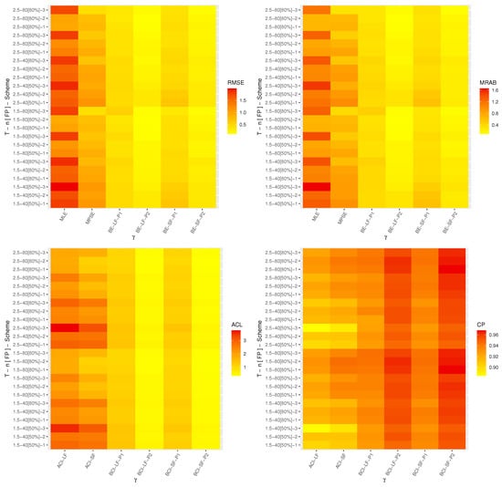
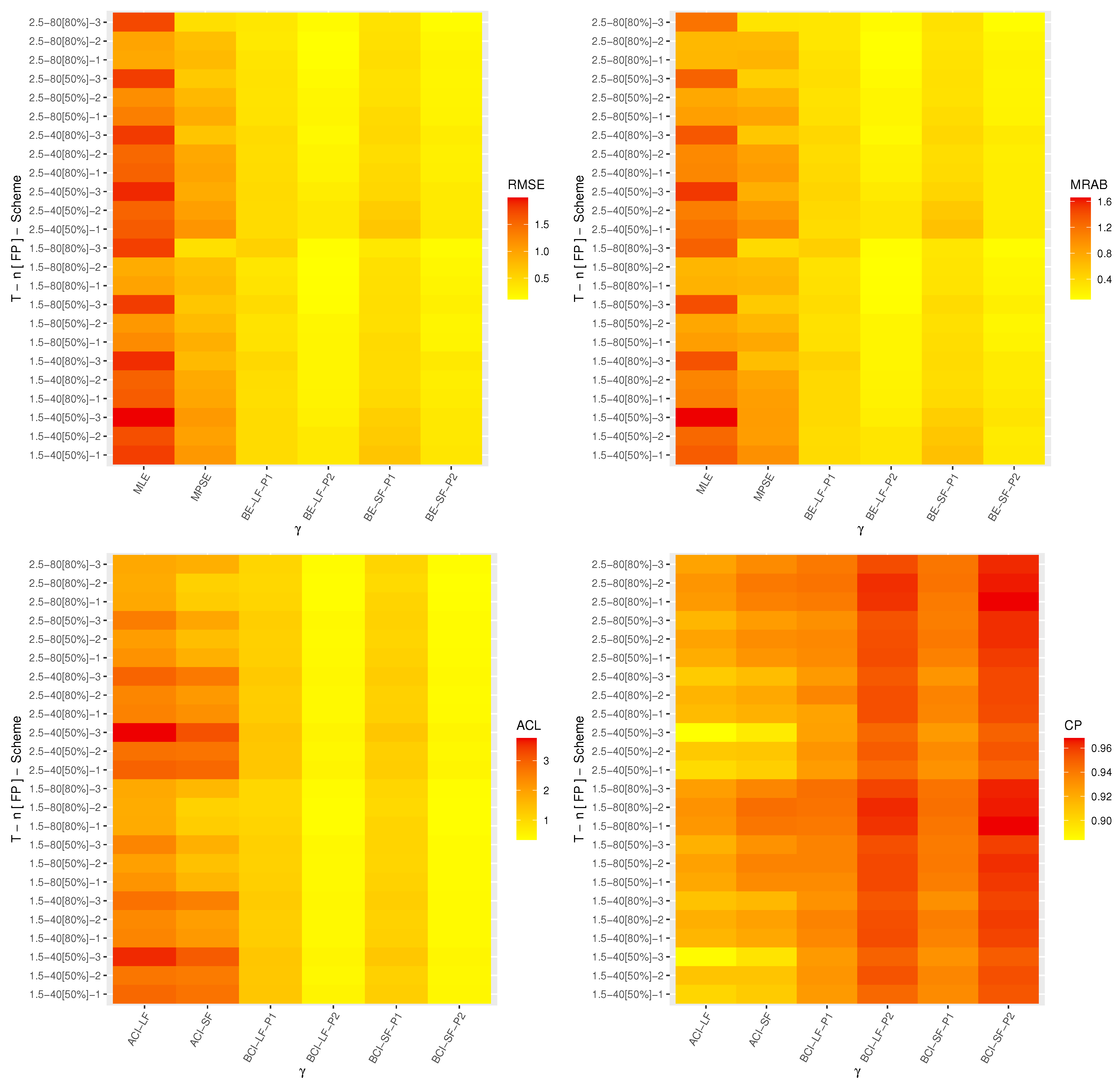
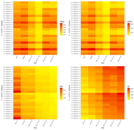
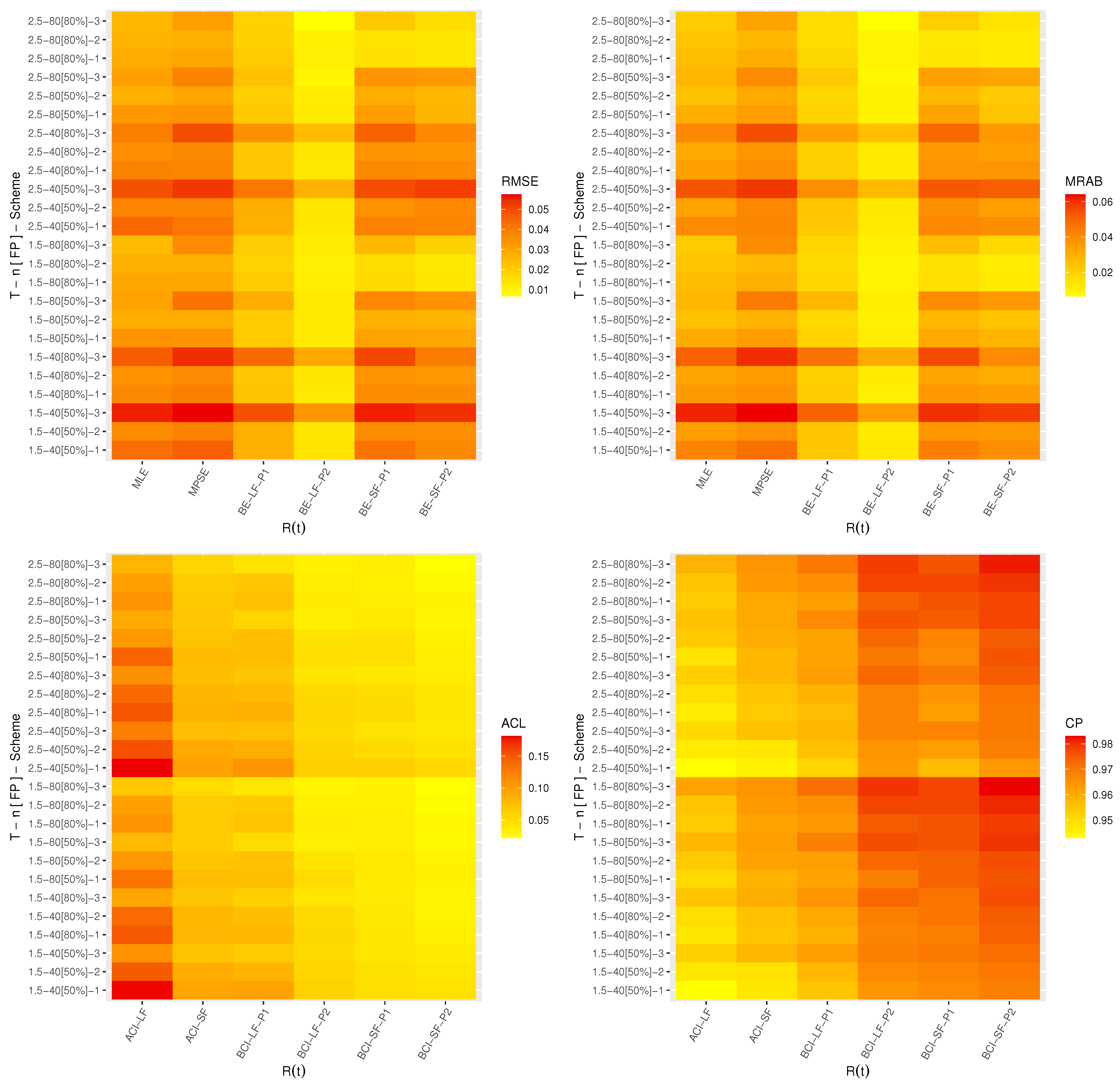
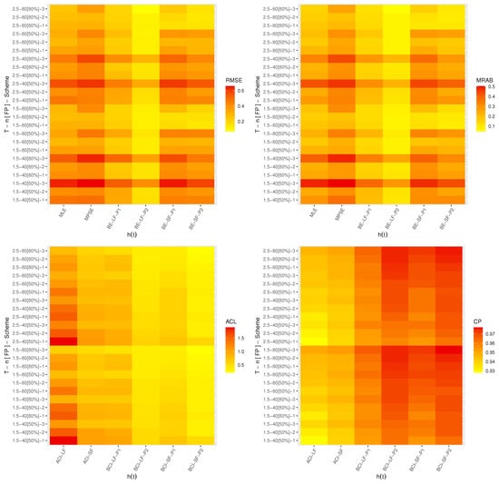
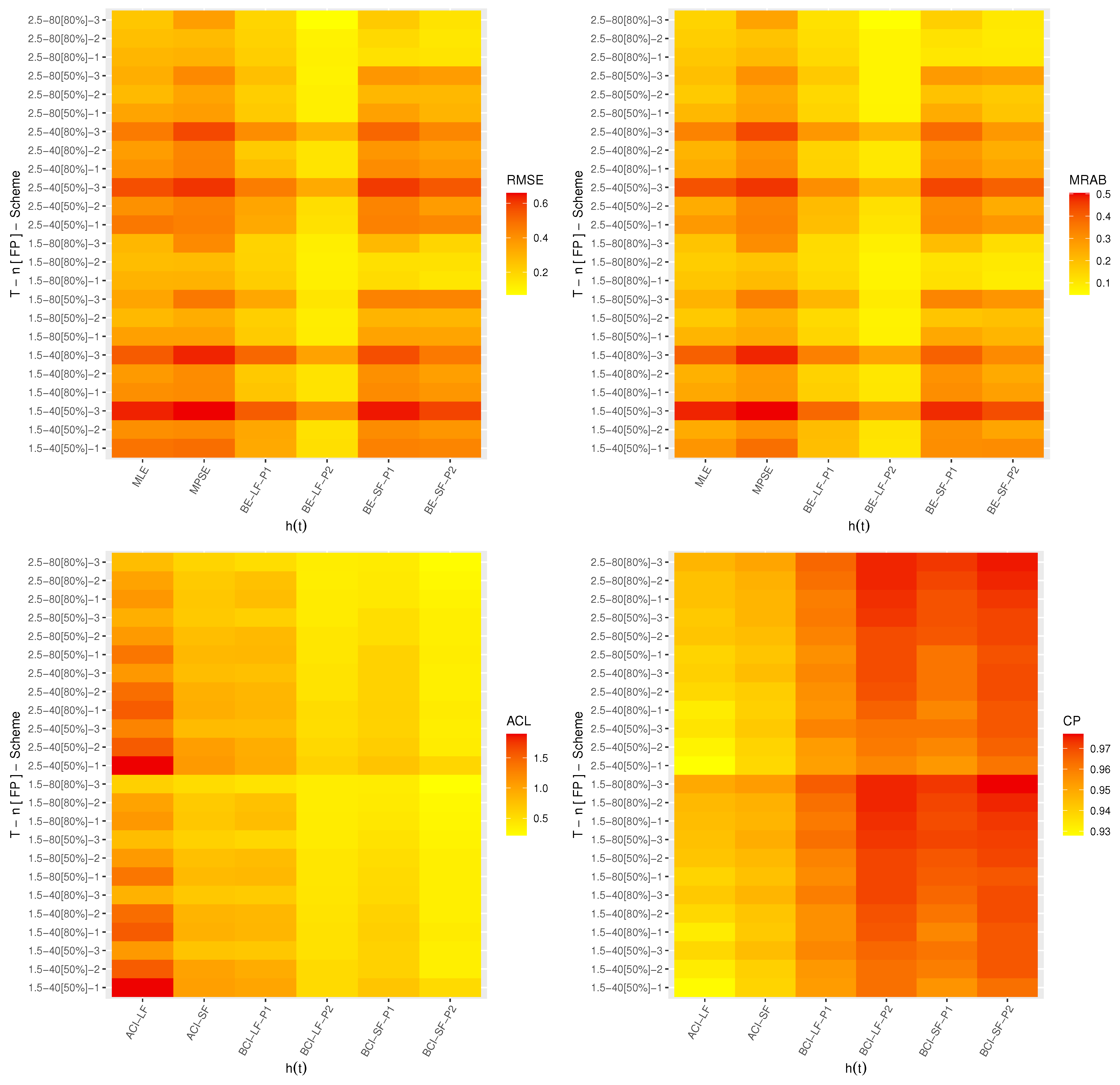
We used the $\mathsf{R}$ 4.2.2 programming software, after installing two useful packages, namely: (i) “$\mathsf{maxLik}$” (by Henningsen and Toomet [29]) and (ii) “$\mathsf{coda}$” (by Plummer et al. [32]). A heat map diagram is a data visualization technique that depicts the magnitude of a phenomenon in two dimensions, where the values are encoded in colors.

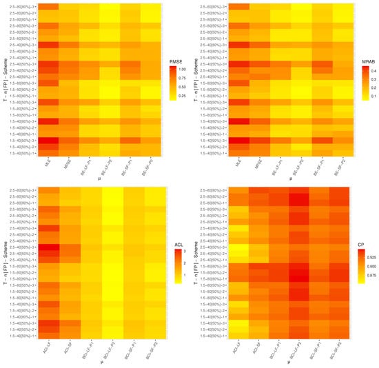
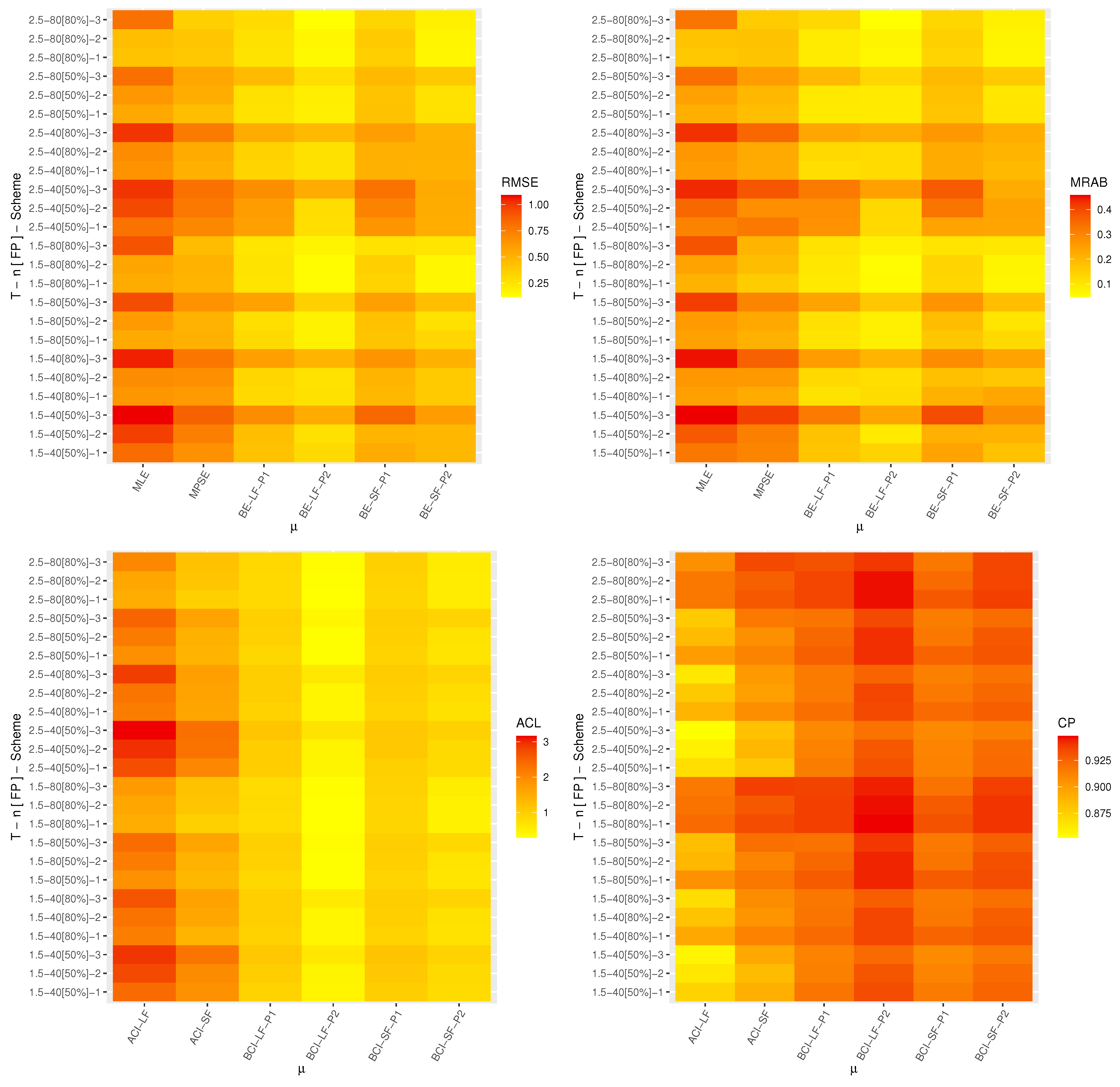
Thus, the simulation outputs of $\mu$, $\gamma$, $R(t)$, and $h(t)$ are shown via the heat maps in Figure 2, Figure 3, Figure 4 and Figure 5, respectively. In the Supplementary File, the simulation tables are presented. In each heat map, “$\mathsf{x}-\mathsf{lab}$” displays the proposed point and interval estimation methods, while “$\mathsf{y}-\mathsf{lab}$” displays the proposed censoring, which is referred to as the “$T-n\left[\mathrm{FP}\right]$-Scheme”. In the elegant heat map, the simulated values of the RMSE, MRAB, ACL, or CP are specified using colors from yellow (smallest values) to red (highest values). For simplification, based on the Prior 1 set (say P1), several notations were used such as “BE-LF-P1” for the Bayes results from the likelihood function; “BE-SF-P1” for the Bayes results from the product of spacings function; “BCI-LF-P1” for the BCI estimates from the likelihood function; and “BE-SF-P1” for the BCI estimates from the product of spacings function.

4.2. Simulation Discussions

This subsection discusses several evaluations of the execution of the suggested inferential techniques. From Figure 2, Figure 3, Figure 4 and Figure 5, we list the following observations:

• All derived estimates of $\mu$, $\gamma$, $R(t)$, or $h(t)$ behaved satisfactorily in terms of the minimum RMSE, MRAB, and ACL values, as well as the highest CPs.
• As n increased, the acquired point (or interval) estimates were good. An identical pattern was noted when ${\sum }_{i=1}^r{R}_i$ (or $n-r$) narrowed down.
• As T increased, the RMSEs and MRABs for various estimates of $\mu$ and $\gamma$ increased, while those of $R(t)$ and $h(t)$ decreased.
• As T increased, the ACLs for various estimates of $\mu$, $\gamma$, $R(t)$, and $h(t)$ increased, while their CPs decreased.
• All Bayes results against Prior 2 were superior compared to Prior 1. This was to be expected given that Prior 2’s variance was lower than Prior 1’s.
• In most cases, the CPs of the calculated asymptotic (or Bayes) intervals of $\mu$, $\gamma$, $R(t)$, or $h(t)$ were near the specified nominal level.
• Comparing the suggested schemes, it was observed in the point inference that the unknown parameters $\mu$ and $\gamma$ behaved well using Schemes 1 “left censoring” and 3 “right censoring”, respectively, whereas $R(t)$ and $h(t)$ behaved well using Scheme 2 “middle censoring”.
• Comparing the suggested schemes, it was observed in the interval inference that the unknown parameters $\mu$ and $\gamma$ behaved well using Schemes 1 “left censoring” and 2 “middle censoring”, respectively, whereas $R(t)$ and $h(t)$ behaved well using Scheme 3 “left censoring”.
• Comparing the point estimation methodologies, in most tests, it was noted that:

  (i)

  In a classical setup, the estimates of $\mu$ and $\gamma$ obtained from the product of spacings approach, as well as those of $R(t)$ and $h(t)$ obtained from the likelihood approach performed satisfactorily compared to the others.

  (ii)

  In a Bayes setup, the estimates of $\mu$, $\gamma$, $R(t)$, and $h(t)$ obtained from the likelihood approach performed superior to others.

• Comparing the interval estimation methodologies, in most tests, it was noted that:

  (i)

  In a classical setup, the ACIs of $\mu$, $\gamma$, $R(t)$, and $h(t)$ developed from the product of spacings function performed better than the others.

  (ii)

  In a Bayes setup, the BCIs of $\mu$ developed from the likelihood function, as well as those of $\gamma$, $R(t)$, and $h(t)$ obtained from the product of spacings function performed superior to the others.

• The estimated duration of a study based on Scheme 1 (or 2) is known to be larger than that of any other, and hence, the sample acquired under the AT2PHC plan provided more extra information than those produced using any other strategy.
• As a result, from the AT2PHC plan, the Bayes technique through the MH-G algorithm is recommended to estimate the PE’s parameters of life.

5. Optimal Progressive Fashions

In the context of reliability trials, the practitioner is concerned with selecting the best censoring scheme from a set of all feasible censoring strategies. Thus, selecting the best progressive censoring fashions has received much attention in the statistical literature; for example, see Ng et al. [33], Pradhan and Kundu [34], and Dey and Elshahhat [28], among others. Determining the most-appropriate sampling strategy means discovering the progressive mechanism among all potential progressive censoring plans that provides the greatest knowledge about the unknown parameters. In

Table 1. Optimal T2PC criteria.

Criterion	Method
${\mathcal{O}}_1$	$\mathrm{Maximize}\mathrm{trace}({\mathbf{I}}_{2\times 2}(\widehat{\mathsf{\Omega }}))$
${\mathcal{O}}_2$	$\mathrm{Minimize}\mathrm{trace}({\mathbf{I}}_{2\times 2}^{-1}(\widehat{\mathsf{\Omega }}))$
${\mathcal{O}}_3$	$\mathrm{Minimize}det({\mathbf{I}}_{2\times 2}^{-1}(\widehat{\mathsf{\Omega }}))$
${\mathcal{O}}_4$	$\mathrm{Minimize}\widehat{var}(log({\widehat{\Psi }}_{\xi })),0<\xi <1$

, various optimality criteria, which have been widely used in the literature, are used to assist us in choosing the most-optimum T2PC plan.

Regarding the criterion ${\mathcal{O}}_1$, for given $(T,n,m)$ and $(R_i,x_i),i=1,2,\dots ,r$, we sought to maximize the main diagonal members of the estimated Fisher information acquired from the likelihood and product of spacings approaches. Similarly, according to ${\mathcal{O}}_i,i=2,3$, we aimed to minimize the trace and determinant of the estimated VC matrix, respectively, obtained from the proposed frequentist approaches. Moreover, ${\mathcal{O}}_4$ serves to reduce the variance of the log-MLE (or log-MPSE) of the $\xi$th quantile, denoted by $\widehat{var}(log({\widehat{\Psi }}_{\xi }))$, such that

$$\begin{array}{c}\hfill log({\widehat{\Psi }}_{\xi })=log\left\{{\mu }^{-1}\left[log(\gamma )-log(-log(\xi -(\xi -1)e^{-\gamma }))\right]\right\},0<\xi <1,\end{array}$$

where the delta method was also considered here to obtain $\widehat{var}(log({\widehat{\Psi }}_{\xi }))$. To pick the optimum T2PC design, obviously, one should obtain the censoring pattern that gives the lowest values of criteria ${\mathcal{O}}_i,i=2,3,4$ and the highest value of criterion ${\mathcal{O}}_1$.

6. Chemical Engineering Applications

This section presents two applications, to illustrate how the proposed approaches may be applied in a practical context, based on different real-world datasets from the chemical engineering area.

6.1. Cumin Essential Oil

In this application, we shall analyze an actual dataset representing the primary chemical constituent (called cuminaldehyde) of cumin essential oil (CEO). Cumin oil is produced from the seeds harvested from flowering herbaceous plant. Industrially, CEO is commonly used for food and flavor preservation purposes, such as to modify the flavor of herbs, spices, dill, biscuits, cake flavors, etc. Panahi [35] first collected the cuminaldehyde experimental data with $n=24$ of CEO utilizing a distillation pilot plant; see

Table 2. Cuminaldehyde data of cumin essential oil.

33.86	36.55	37.89	37.96	39.60	42.46	43.54	44.81	45.23	47.58	48.67	49.85
50.54	50.91	53.98	55.89	57.87	59.39	64.98	66.68	66.76	67.57	68.45	70.89

.

To verify whether the PE distribution is an adequate model for the CEW dataset, the MLEs (with their standard errors (St.Es)) of $\mu$ and $\gamma$ were calculated first to obtain the Kolmogorov–Smirnov (KS) statistic with its p-value. However, from Table 2, the values of $\widehat{\mu }$, $\widehat{\gamma }$, and KS (p-value) were 0.1041 (0.0167), 124.55 (91.536), and 0.1021 (0.942), respectively. Since the estimated P-value was far from the specified significance percent (5%), then the PE distribution fit the CED data quite well. Three plots were also investigated to check the fit result, namely: (iii) estimated/empirical PE reliability function, (i) estimated/empirical scaled total-time-on-test (TTT) transform, (ii) histogram of the given data with the estimated PDFs, and (iii) contour diagram for the log-likelihood of $\mu$ and $\gamma$; see Figure 6. For clarity, the fit RF (or TTT) line in Figure 6a,b is shown by a solid red line, and the $\mathsf{x}$-point in Figure 6c represents the acquired MLEs of $\mu$ and $\gamma$. Also, in Figure 6c, the heat-color from red to yellow to white represents the region where the best estimate is obtained. As a result, Figure 6a offers that the fit RF line captured the empirical RF line adequately; Figure 6b indicates that the CEO dataset has an increasing HRF; Figure 6c shows that the MLEs $\widehat{\mu }$ and $\widehat{\gamma }$ used in the KS calculations exist and were unique.

From the full CEO dataset, in

Table 3. Various AT2PHC samples from the CEO data.

Sample	Scheme	$\mathbf{T}(\mathbf{m})$	${\mathit{R}}_{\mathit{r}}$	Data
${\mathcal{S}}_1$	$(3^4,0^8)$	40 (2)	6	33.86, 39.60, 42.46, 44.81, 45.23, 47.58, 48.67, 50.91, 53.98, 55.89, 57.87, 59.39
${\mathcal{S}}_2$	$(0^4,3^4,0^4)$	46 (7)	3	33.86, 36.55, 37.89, 37.96, 39.60, 43.54, 45.23, 47.58, 48.67, 57.87, 59.39, 66.76
${\mathcal{S}}_3$	$(0^8,3^4)$	51 (12)	0	33.86, 36.55, 37.89, 37.96, 39.60, 42.46, 43.54, 44.81, 45.23, 48.67, 49.85, 50.54

, three AT2PHC samples with $r=12$ were generated based on various options of T and $\mathbf{R}$. For each $\mathcal{S}$i sample for $i=1,2,3$, the acquired point estimates (with their St.Es) and 95% interval estimates (with their interval widths (IWs)) obtained by both classical and Bayes methodologies of $\mu$, $\gamma$, $R(t)$, and $h(t)$ (at $t=50$) were evaluated and are provided in

Table 4. Estimates of $\mu$, $\gamma$, $R(t)$, and $h(t)$ from the CEO data.

Sample	Par.	MLE		MCMC-LF		ACI-LF			BCI-LF
		MPSE		MCMC-SF		ACI-SF			BCI-SF
		Est.	St.E	Est.	St.E	Lower	Upper	IW	Lower	Upper	IW
${\mathcal{S}}_1$	$\mu$	0.0904	0.0059	0.0904	0.0010	0.0788	0.1019	0.0231	0.0902	0.0906	0.0004
		0.0770	0.0062	0.0770	0.0010	0.0647	0.0892	0.0245	0.0768	0.0772	0.0004
	$\gamma$	92.367	14.332	92.366	0.0014	64.276	120.46	56.180	92.366	92.367	0.0004
		47.347	8.8766	47.342	0.0014	29.949	64.744	34.796	47.342	47.343	0.0004
	$R(50)$	0.6350	0.0900	0.6351	0.0184	0.4587	0.8114	0.3527	0.6314	0.6387	0.0073
		0.6356	0.0887	0.6349	0.0183	0.4618	0.8094	0.3476	0.6313	0.6384	0.0071
	$h(50)$	0.0523	0.0106	0.0523	0.0021	0.0316	0.0731	0.0415	0.0519	0.0528	0.0008
		0.0445	0.0095	0.0446	0.0019	0.0260	0.0631	0.0371	0.0443	0.0450	0.0007
${\mathcal{S}}_2$	$\mu$	0.0814	0.0075	0.0814	0.0010	0.0667	0.0960	0.0293	0.0812	0.0816	0.0004
		0.0690	0.0056	0.0690	0.0010	0.0579	0.0800	0.0221	0.0688	0.0692	0.0004
	$\gamma$	50.874	12.692	50.874	0.0014	25.999	75.750	49.751	50.874	50.875	0.0004
		28.629	3.6603	28.629	0.0014	21.455	35.803	14.348	28.628	28.629	0.0004
	$R(50)$	0.5813	0.0909	0.5813	0.0183	0.4032	0.7594	0.3563	0.5777	0.5849	0.0072
		0.5972	0.0896	0.5972	0.0185	0.4217	0.7727	0.3511	0.5935	0.6007	0.0072
	$h(50)$	0.0510	0.0103	0.0510	0.0019	0.0308	0.0713	0.0405	0.0506	0.0514	0.0008
		0.0423	0.0086	0.0423	0.0017	0.0254	0.0592	0.0338	0.0420	0.0427	0.0007
${\mathcal{S}}_3$	$\mu$	0.1114	0.0053	0.1114	0.0010	0.1010	0.1217	0.0207	0.1112	0.1116	0.0004
		0.0951	0.0051	0.0951	0.0010	0.0852	0.1051	0.0199	0.0950	0.0953	0.0004
	$\gamma$	162.83	12.642	162.83	0.0014	138.05	187.60	49.557	162.83	162.83	0.0004
		78.358	4.0709	78.358	0.0014	70.379	86.337	15.958	78.358	78.358	0.0004
	$R(50)$	0.4628	0.0827	0.4629	0.0168	0.3008	0.6249	0.3240	0.4595	0.4661	0.0066
		0.4899	0.0849	0.4899	0.0174	0.3234	0.6563	0.3328	0.4864	0.4932	0.0067
	$h(50)$	0.0803	0.0105	0.0803	0.0021	0.0597	0.1009	0.0412	0.0799	0.0807	0.0008
		0.0667	0.0097	0.0667	0.0020	0.0477	0.0857	0.0380	0.0663	0.0671	0.0008

.

Since we lacked the prior information for $\mu$ and $\gamma$ from the CEO data, as pointed out by Louzada-Neto et al. [2], Jeffrey’s and improper gamma priors were used to update $\mu$ and $\gamma$, respectively, where $({\alpha }_1,{\alpha }_2)=(1,0.0001)$. The estimated maximum likelihood and maximum product of spacings values of $\mu$ and $\gamma$ were considered as starting guesses to operate the MCMC sampler in the Bayes LF-based and Bayes SF-based methods, respectively. After eliminating the first 10,000 iterations from the total simulated 50,000 iterations, the BE-LF and BE-SF estimates, as well as the 95% BCI-LF and BCI-SF estimates of $\mu$, $\gamma$, $R(t)$, and $h(t)$ were acquired. It is noted, from Table 4, that the estimates obtained from the MLE (or MPSE) method were quite close to those obtained from the MCMC-LF (or MCMC-SF) method. Similar patterns are also noted if one compares the ACI-LF (or ACI-SF) with the BCI-LF (or BCI-SF) techniques. In terms of the smallest St.E and IW values, the Bayes MCMC-LF (or MCMC-SF) estimates provided more accurate results than the MLE (or MPSE) approach.

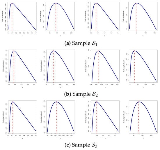
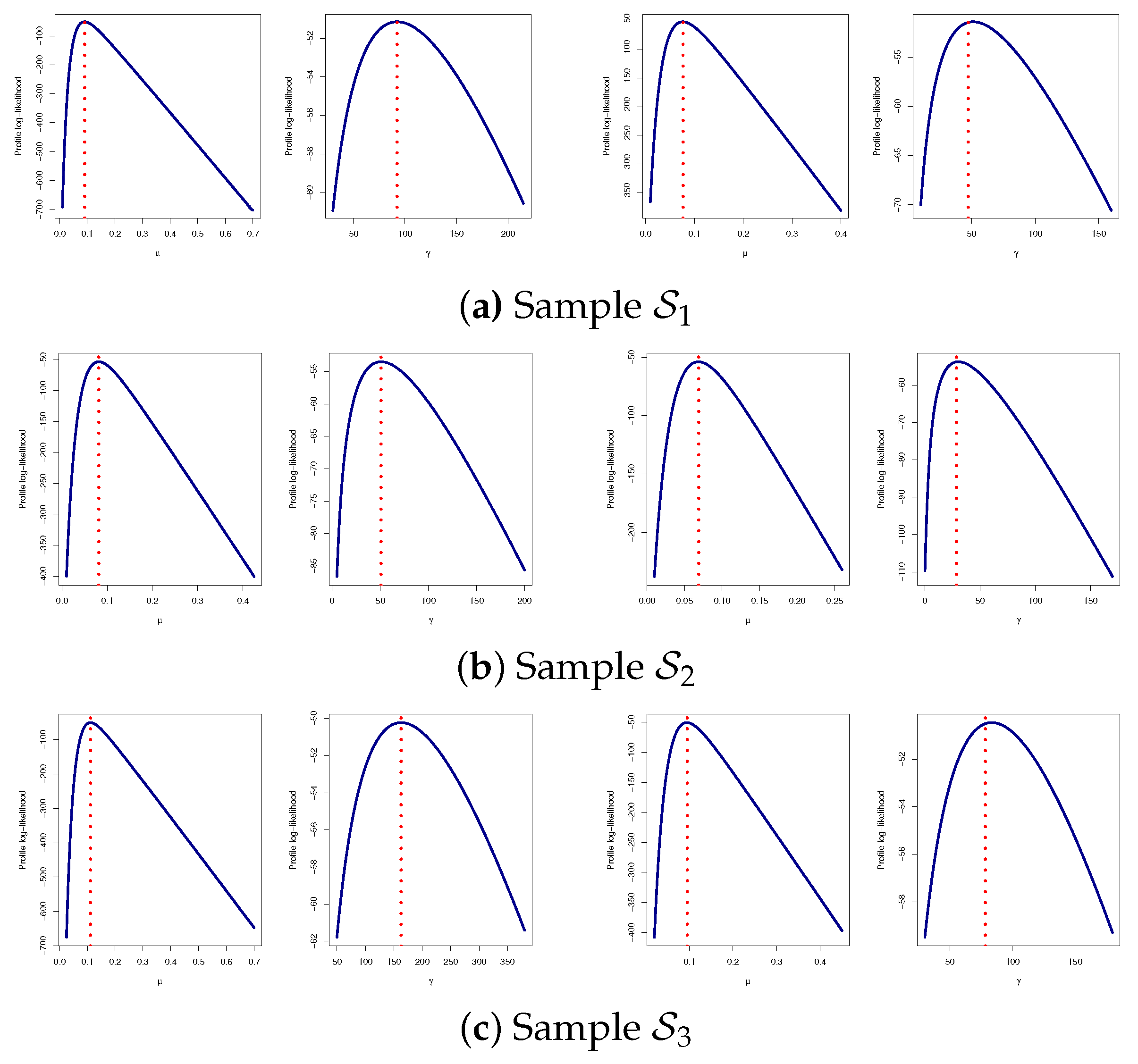
To guarantee the existence and uniqueness of the ML (or MPS) estimates, developed from the CEO data, the profile log-LF and the profile log-SF of $\mu$ and $\gamma$ are displayed in Figure 7. For instance, the observed log-LF (or log-SF) curve is displayed with a solid blue horizontal line, whereas the acquired MLE (or MPSE) value is shown by a red dotted vertical line. Figure 7 shows that the proposed MLEs and MPSEs of $\mu$ and $\gamma$ exist and were unique, as well as supports their estimated values provided in Table 4.

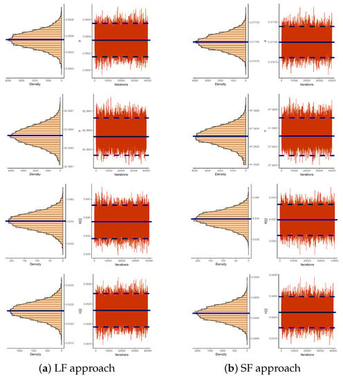
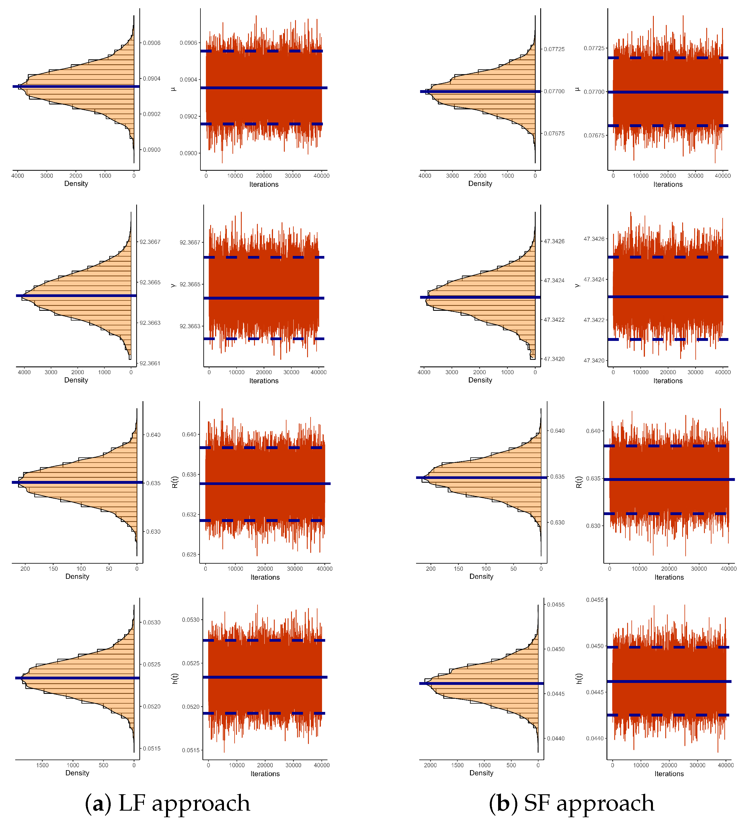
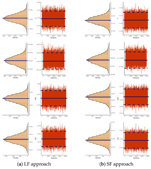
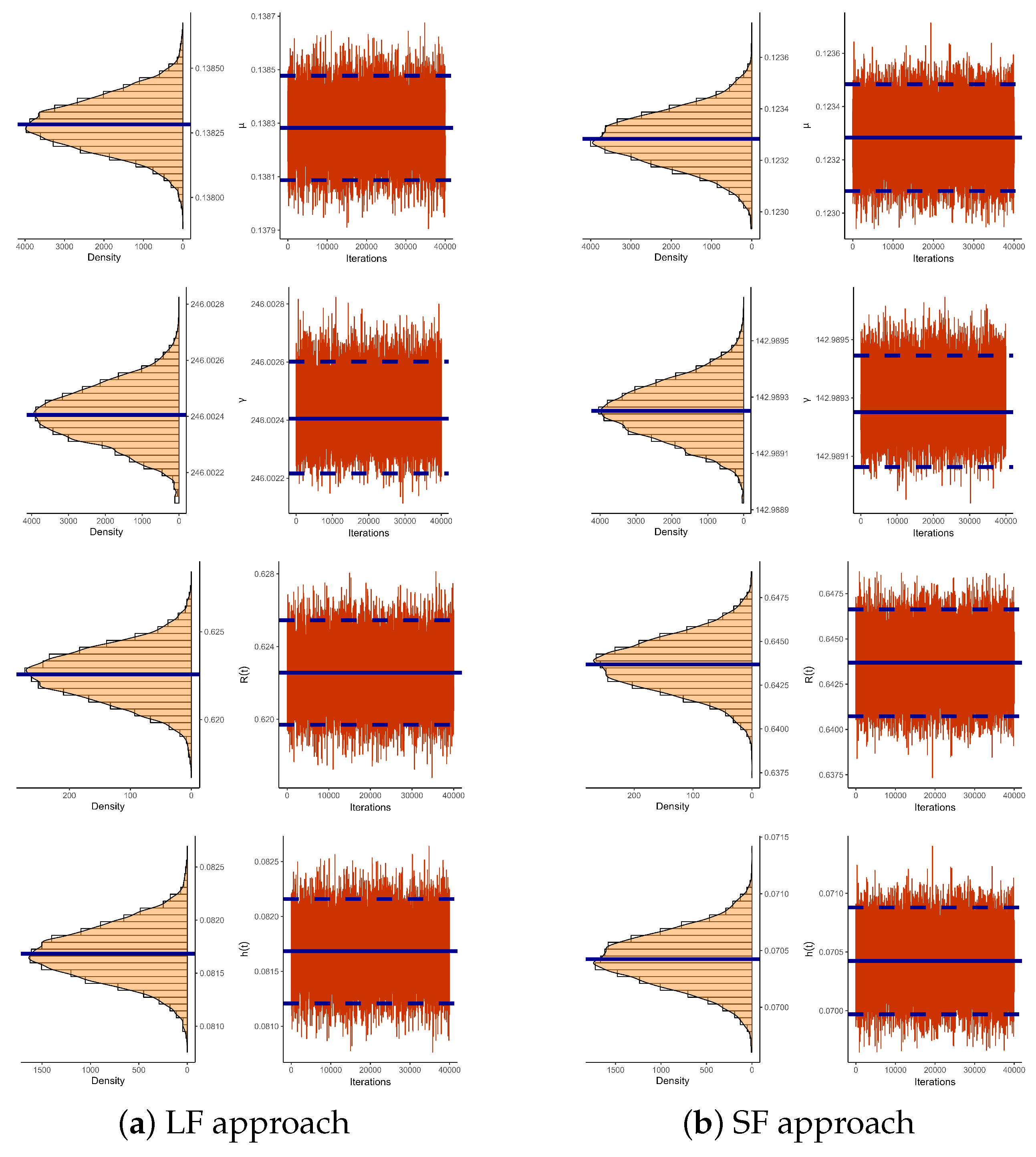
From Sample ${\mathcal{S}}_1$ (as an example), to demonstrate the performance of the simulated Markovian samples of $\mu$, $\gamma$, $R(t)$, and $h(t)$, trace, as well as histogram diagrams are shown in Figure 8, while the same types of plots for the same unknown quantities based on Samples ${\mathcal{S}}_i,i=2,3$ are available as Supplementary Sources. For clarification, in each trace plot, the sample mean and two limits of the 95% BCI are shown by solid and dashed, respectively, blue horizontal lines, whereas the sample mean is also represented by a blue solid line in each density plot. Figure 8 shows that the estimated marginal PDFs, developed from the MCMC-LF (or MCMC-SF) method, of $\mu$, $\gamma$, $R(t)$, or $h(t)$ were fairly symmetric. It also indicates that the burn-in had an efficient size to abandon the impact of the starting guesses and to mix the simulated samples adequately.

Again, using Sample ${\mathcal{S}}_1$ (as an example), some common statistics, namely: the mean, mode, first quartile ($Q_1$), third quartile ($Q_3$), standard deviation (SD), and skewness (Sk.), based on 40,000 MCMC outputs of $\mu$, $\gamma$, $R(t)$, and $h(t)$, are computed and listed in

Table 5. Summary for MCMC variates of $\mu$, $\gamma$, $R(t)$, and $h(t)$ from the CEO data.

Sample	Par.	Mean	Mode	${\mathit{Q}}_1$	${\mathit{Q}}_2$	${\mathit{Q}}_3$	SD	Sk.
${\mathcal{S}}_1$	$\mu$	0.0904	0.0902	0.0903	0.0904	0.0904	0.0001	0.0187
		0.0770	0.0771	0.0769	0.0770	0.0771	0.0001	0.0493
	$\gamma$	92.366	92.366	92.366	92.366	92.367	0.0001	0.0106
		47.342	47.342	47.342	47.342	47.342	0.0001	−0.0746
	$R(50)$	0.6351	0.6374	0.6338	0.6351	0.6363	0.0018	−0.0188
		0.6349	0.6333	0.6336	0.6349	0.6361	0.0018	−0.0494
	$h(50)$	0.0523	0.0521	0.0522	0.0523	0.0525	0.0002	0.0175
		0.0446	0.0448	0.0445	0.0446	0.0447	0.0002	0.0490

. In this table, the calculated statistics developed from the MCMC-LF and MCMC-SF methods are listed in the first and second rows, respectively. It also supports the same findings shown in Table 4 and Figure 8. Additionally, the same MCMC characteristics of $\mu$, $\gamma$, $R(t)$, and $h(t)$ based on Samples ${\mathcal{S}}_2$ and ${\mathcal{S}}_3$ are computed and reported in the Supplementary File also.

Following Section 5, we shall deal with the issue of finding the ideal censoring strategy from all available censoring designs, also investigated using the CEO data. Therefore, the suggested optimum criteria, presented in Table 1, were evaluated through the MLE and MPSE values of $\mu$ and $\gamma$.

Table 6. Fit T2PC criteria from the CEO data.

Sample	${\mathcal{O}}_1$	${\mathcal{O}}_2$	${\mathcal{O}}_3$	${\mathcal{O}}_4$
$\mathit{\xi }\to$				0.3	0.6	0.9
MLE
${\mathcal{S}}_1$	41,866.25	205.406	0.00491	6.75192	9.83368	17.5193
${\mathcal{S}}_2$	40,860.91	161.084	0.00394	7.84087	12.5272	26.0732
${\mathcal{S}}_3$	40,886.40	159.826	0.00391	3.82899	5.30541	8.71828
MPSE
${\mathcal{S}}_1$	43,115.80	78.7949	0.00183	8.91487	13.9230	27.4149
${\mathcal{S}}_2$	41,933.12	16.5722	0.00040	10.5710	17.3449	35.2131
${\mathcal{S}}_3$	40,931.40	13.3981	0.00032	5.19858	7.56814	13.1462

shows that the censoring plan used in $S_1$ based on the criterion ${\mathcal{O}}_1$, while the censoring plan used in $S_3$ according to the given criteria ${\mathcal{O}}_i,i=2,3,4$ were the optimum censoring compared to the others.

6.2. Coating Weights of Iron Sheets

This application offers the analysis of chemistry data, representing the coating weights of iron sheets, collected during January–March 2018 by the Aluminium Africa Limited (ALAF) (commercially) industry in Tanzania. Here, from the ALAF industry, we shall provide a dataset consisting of 72 observations on the coating weight (in gm/m${}^2$); see

Table 7. Coating weights of iron sheets from the ALAF industry.

28.7	29.4	30.4	31.6	31.8	32.7	32.9	33.2	33.2	33.6	33.7	34.0	34.2	34.5	35.6
36.2	36.7	36.8	36.8	37.3	37.8	38.5	38.9	38.9	39.1	39.9	40.1	40.2	40.3	40.5
40.6	40.7	41.2	41.2	41.3	42.3	42.3	42.6	42.8	42.8	42.8	42.8	43.1	44.2	44.9
45.2	45.3	45.4	45.8	46.3	47.1	47.2	47.2	48.2	48.3	48.4	48.5	49.8	50.1	52.6
52.8	54.2	54.5	55.4	55.8	56.8	58.2	58.4	58.7	58.9	59.2	61.2

. Originally, this dataset was first presented by Rao and Mbwambo [36] and reanalyzed later by Fan and Gui [37].

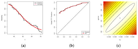
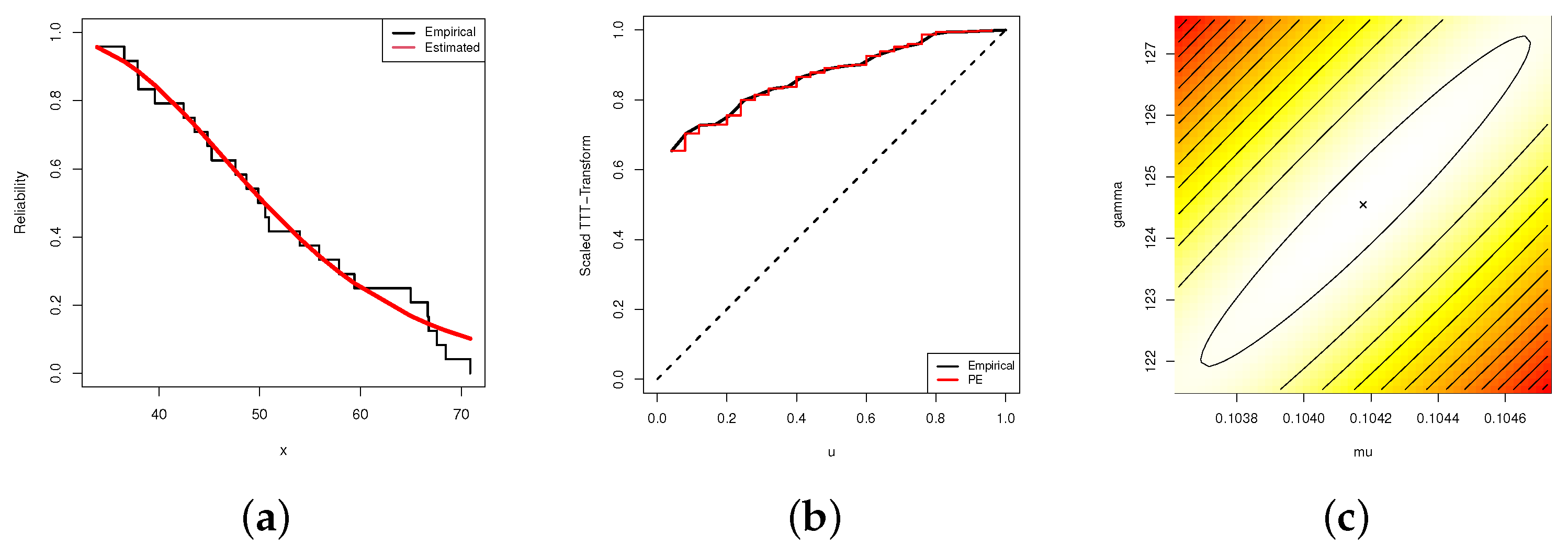
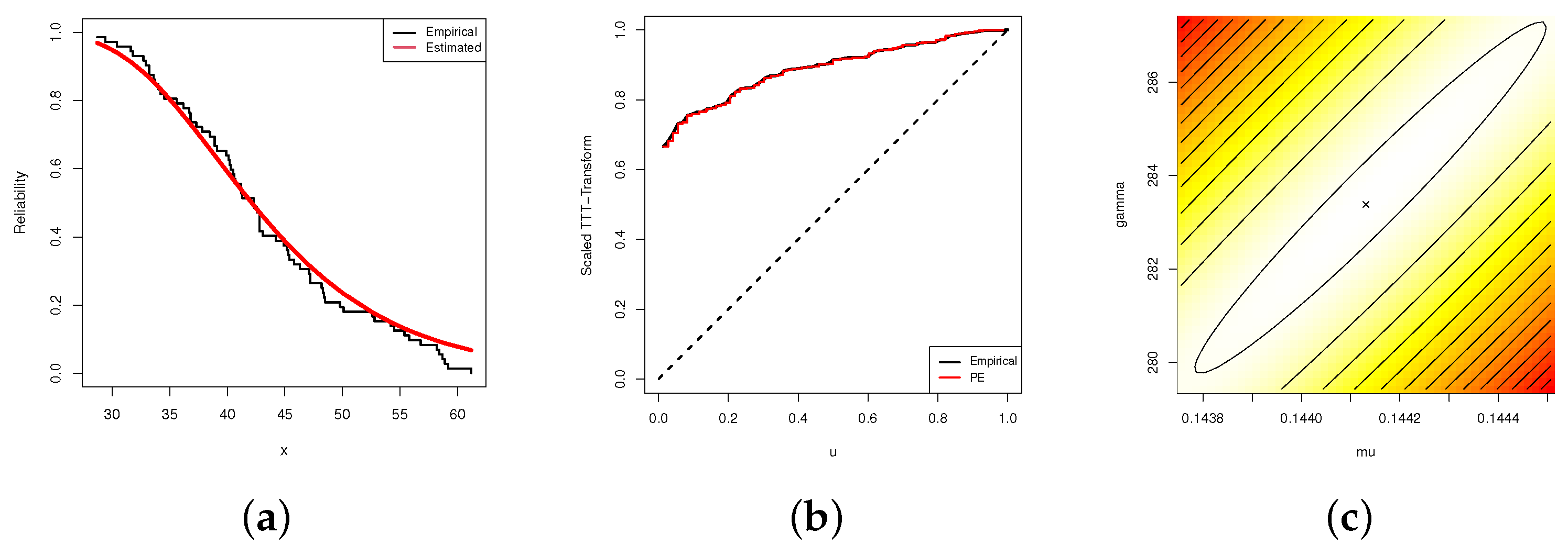
Before proceeding, from Table 7, the estimation results of $\widehat{\mu }$, $\widehat{\gamma }$, and KS (p-value) were 0.1441 (0.0132), 283.37 (139.35), and 0.0715 (0.855), respectively. It is clear that the PE lifetime model fit the coating weights dataset satisfactorily. Again, similar to the three plots depicted on Figure 6, several plots using the complete coating weights data are shown in Figure 9. As we anticipated, Figure 9a indicates that fit RF line supports the fit finding, Figure 9b shows that the coating weights dataset has an increasing HRF, and Figure 9c shows that the acquired MLEs $\widehat{\mu }$ and $\widehat{\gamma }$ exist and were unique also.

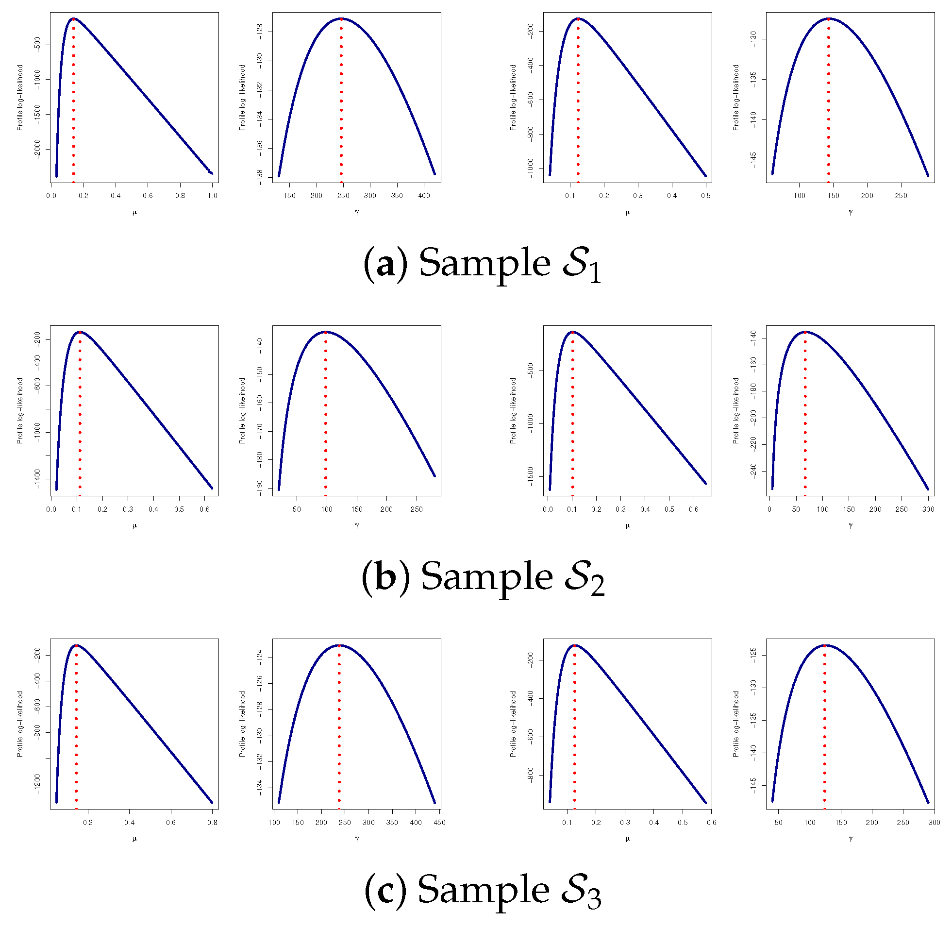
From the entire coating weights data, by performing $m=32$ and various selections of $\mathbf{R}$ and T, three AT2PHC samples are presented in

Table 8. Various AT2PHC samples from the coating weights data.

Sample	Scheme	$\mathit{T}(\mathit{m})$	${\mathit{R}}_{\mathit{r}}$	Data
${\mathcal{S}}_1$	$(5^8,0^{24})$	30 (2)	30	28.7, 29.4, 31.8, 32.9, 33.2, 33.2, 33.6, 33.7, 34.0, 34.2, 34.5,
				35.6, 36.2, 36.7, 36.8, 36.8, 37.3, 37.8, 38.5, 39.1, 39.9, 40.1,
				40.2, 40.3, 40.5, 40.6, 41.2, 41.3, 42.3, 42.6, 42.8, 42.8
${\mathcal{S}}_2$	$(0^{12},5^8,0^{12})$	37 (16)	20	28.7, 29.4, 30.4, 31.6, 31.8, 32.7, 32.9, 33.2, 33.2, 33.6, 33.7,
				34.0, 34.2, 34.5, 36.7, 36.8, 38.5, 39.1, 39.9, 40.1, 40.3, 40.5,
				40.6, 40.7, 42.3, 42.3, 42.6, 44.2, 44.9, 45.2, 45.3, 47.2
${\mathcal{S}}_3$	$(0^{24},5^8)$	42 (30)	10	28.7, 29.4, 30.4, 31.6, 31.8, 32.7, 32.9, 33.2, 33.2, 33.6, 33.7,
				34.0, 34.2, 34.5, 35.6, 36.2, 36.7, 36.8, 36.8, 37.3, 37.8, 38.5,
				38.9, 38.9, 39.1, 39.9, 40.1, 40.6, 40.7, 41.3, 42.3, 46.3

. Both point (with their St.Es) estimates and interval (with their IWs) estimates of $\mu$, $\gamma$, $R(t)$, and $h(t)$ (at $t=40$) were obtained and are listed in

Table 9. Estimates of $\mu$, $\gamma$, $R(t)$, and $h(t)$ from the coating weights data.

Sample	Par.	MLE		MCMC-LF		ACI-LF			BCI-LF
		MPSE		MCMC-SF		ACI-SF			BCI-SF
		Est.	St.E	Est.	St.E	Lower	Upper	IW	Lower	Upper	IW
${\mathcal{S}}_1$	$\mu$	0.1383	0.0035	0.1383	0.0010	0.1314	0.1452	0.0138	0.1381	0.1385	0.0004
		0.1233	0.0036	0.1233	0.0010	0.1162	0.1304	0.0141	0.1231	0.1235	0.0004
	$\gamma$	246.00	6.0398	246.00	0.0014	234.16	257.84	23.676	246.00	246.00	0.0004
		142.99	4.3040	142.99	0.0014	134.55	151.43	16.871	142.99	142.99	0.0004
	$R(40)$	0.6226	0.0508	0.6226	0.0147	0.5231	0.7220	0.1989	0.6197	0.6254	0.0057
		0.6437	0.0517	0.6437	0.0149	0.5423	0.7451	0.2028	0.6407	0.6466	0.0059
	$h(40)$	0.0817	0.0084	0.0817	0.0024	0.0652	0.0982	0.0330	0.0812	0.0822	0.0010
		0.0704	0.0080	0.0704	0.0023	0.0547	0.0861	0.0314	0.0700	0.0709	0.0009
${\mathcal{S}}_2$	$\mu$	0.1122	0.0038	0.1122	0.0010	0.1047	0.1197	0.0150	0.1120	0.1124	0.0004
		0.1019	0.0037	0.1019	0.0010	0.0946	0.1091	0.0145	0.1017	0.1021	0.0004
	$\gamma$	98.137	6.7694	98.137	0.0014	84.869	111.40	26.535	98.137	98.137	0.0004
		67.200	3.7342	67.200	0.0014	59.881	74.519	14.638	67.200	67.200	0.0004
	$R(40)$	0.6682	0.0490	0.6682	0.0147	0.5721	0.7643	0.1922	0.6653	0.6711	0.0058
		0.6811	0.0494	0.6811	0.0145	0.5843	0.7778	0.1935	0.6782	0.6839	0.0057
	$h(40)$	0.0615	0.0073	0.0615	0.0022	0.0472	0.0758	0.0286	0.0610	0.0619	0.0009
		0.0545	0.0069	0.0545	0.0020	0.0410	0.0680	0.0269	0.0541	0.0549	0.0008
${\mathcal{S}}_3$	$\mu$	0.1445	0.0041	0.1445	0.0010	0.1365	0.1525	0.0159	0.1443	0.1447	0.0004
		0.1262	0.0041	0.1262	0.0010	0.1181	0.1343	0.0163	0.1260	0.1264	0.0004
	$\gamma$	237.71	8.6611	237.71	0.0014	220.74	254.69	33.951	237.71	237.71	0.0004
		123.96	4.3089	123.96	0.0014	115.51	132.40	16.891	123.96	123.96	0.0004
	$R(40)$	0.5202	0.0554	0.5202	0.0142	0.4115	0.6288	0.2173	0.5173	0.5229	0.0056
		0.5489	0.0580	0.5489	0.0145	0.4352	0.6626	0.2274	0.5461	0.5517	0.0056
	$h(40)$	0.0979	0.0090	0.0979	0.0023	0.0802	0.1156	0.0354	0.0974	0.0983	0.0009
		0.0826	0.0087	0.0826	0.0022	0.0655	0.0996	0.0340	0.0821	0.0830	0.0008

. Just like the same settings for the Bayes MCMC sampling from the LF-based (or SF-based) method, the Bayes estimates, as well as the associated 95% BCIs were developed. It is evident, from Table 9, in terms of the lowest St.E and IW values, that both the point and interval results developed from the Bayes estimates under the LF-based (or SF-based) approach of $\mu$, $\gamma$, $R(t)$, or $h(t)$ performed better than those obtained from the likelihood (or product of spacings) approach. For each AT2PHC sample in Table 8, the plots of the profile log-LF and the profile log-SF of $\mu$ and $\gamma$ are shown in Figure 10. This supports the estimated values of $\mu$ and $\gamma$ presented in Table 9 and shows that the acquired maximum likelihood and maximum product of spacings of $\mu$ and $\gamma$ exist and were unique.

Both the density and trace plots using sample ${\mathcal{S}}_1$ (as an example) are plotted and displayed in Figure 11. This proves that the MCMC-LF and MCMC-SF techniques converged well and that the simulated marginal density estimates of all unknown quantities behaved almost symmetrically. The same statistics reported in Table 5, based on 40,000 MCMC outputs of $\mu$, $\gamma$, $R(t)$, or $h(t)$ from ${\mathcal{S}}_1$ (as an example), were also obtained from the coating weights data and are presented in

Table 10. Summary for MCMC variates of $\mu$, $\gamma$, $R(t)$, and $h(t)$ from the coating weights data.

Sample	Par.	Mean	Mode	${\mathit{Q}}_1$	${\mathit{Q}}_2$	${\mathit{Q}}_3$	SD	Sk.
${\mathcal{S}}_1$	$\mu$	0.1383	0.1382	0.1382	0.1383	0.1383	0.0001	0.0293
		0.1233	0.1234	0.1232	0.1233	0.1234	0.0001	−0.0197
	$\gamma$	246.00	246.00	246.00	246.00	246.00	0.0001	0.0461
		142.99	142.99	142.99	142.99	142.99	0.0001	0.0729
	$R(40)$	0.6226	0.6234	0.6216	0.6226	0.6236	0.0015	−0.0290
		0.6437	0.6427	0.6427	0.6437	0.6447	0.0015	0.0193
	$h(40)$	0.0817	0.0815	0.0815	0.0817	0.0818	0.0002	0.0274
		0.0704	0.0706	0.0703	0.0704	0.0706	0.0002	−0.0208

. The estimated statistics from the MCMC-LF and MCMC-SF techniques are presented in the first and second rows in Table 10, respectively. Other density and trace plots based on samples ${\mathcal{S}}_i,i=2,3$, as well as their vital statistics, were also obtained and are reported in the Supplementary File.

In

Table 11. Fit T2PC criteria from the coating weights data.

Sample	${\mathcal{O}}_1$	${\mathcal{O}}_2$	${\mathcal{O}}_3$	${\mathcal{O}}_4$
$\mathit{\xi }\to$				0.3	0.6	0.9
MLE
${\mathcal{S}}_1$	84,025.63	36.4797	0.00043	0.92111	1.24319	1.96602
${\mathcal{S}}_2$	89,273.53	45.8243	0.00051	1.36940	1.97747	3.45105
${\mathcal{S}}_3$	64,688.44	75.0153	0.00116	0.99059	1.34004	2.12883
MPSE
${\mathcal{S}}_1$	80,825.40	10.5244	0.00013	1.22241	1.70355	2.80635
${\mathcal{S}}_2$	87,280.77	13.9442	0.00016	1.72264	2.55586	4.57677
${\mathcal{S}}_3$	61,339.85	18.5668	0.00030	1.38045	1.94120	3.23457

, through the MLE and MPSE values of $\mu$ and $\gamma$ developed from coating weights data, the suggested optimum criteria in Section 5 were evaluated. It shows that the censoring plan used in $S_2$ is the optimum censoring compared to the others based on all given criteria ${\mathcal{O}}_i,i=2,3,4$.

In summary, the analysis outcomes of the offered estimates using the complete cumin essential oil and coating weights of iron sheets datasets furnished a good investigation of the Poisson–exponential lifetime model.

7. Conclusions

A new two-parameter Poisson–exponential distribution for data modeling with an increasing failure rate was introduced to address several vital and critical phenomena in various sectors, such as medical, engineering, chemistry, and other fields. A statistical investigation, using an adaptive progressively Type-II hybrid censored strategy, through the maximum likelihood, maximum product of spacings, and Bayes inferential approach of the unknown Poisson–exponential’s parameters of life was presented in this study. From the frequentist approach, the approximate confidence interval of each unknown quantity was also created. From the squared error loss, Bayes point/credible estimators via both the product of spacings and likelihood functions of the unknown parameters were proposed when Jeffrey’s and gamma prior assumptions were available. It should be emphasized that the Bayes estimators cannot be acquired in closed forms, but may be determined via numerical integration; hence, the Markov Chain Monte Carlo technique was utilized. Various numerical examinations were performed to test the performance of the acquired estimators while taking into account different effective sample sizes and censoring procedures. The Monte Carlo results showed that the product of spacings approach was better compared to the likelihood approach in the classical viewpoint, while the Bayes-likelihood-based approach was better compared to the product of spacings approach in the Bayesian viewpoint, in order to derive the point and/or interval estimate of the objective parameter. The best progressive censoring strategies were displayed, and certain optimality criteria were investigated. To assess how the offered estimators performed in practice, two actual datasets taken from the chemical engineering domain were examined. The data analysis stated that the proposed model performed well in the presence of incomplete data, such as adaptive progressively Type-II hybrid censored data. Moreover, we extended some relevant works in the literature that can be easily obtained as special cases, such as: Gitahi et al.’s [6] results when $T\to \infty$; Arabi Belaghi et al.’s [7] results when $R_i,i=1,2,\dots ,m-1,$ and $T\to \infty$; the results of Singh et al. [3], as well as Rodrigues et al. [4] when $R_i,i=1,2,\dots ,m,$ and $T\to \infty$. In the future research, the inferential methods developed in this study can be easily extended to incorporate competing risks or acceleration life test studies.

References

- Cancho, V.G.; Louzada-Neto, F.; Barriga, G.D. The Poisson–exponential lifetime distribution. Comput. Stat. Data Anal. 2011, 55, 677–686. [Google Scholar] [CrossRef] [Scilit]
- Louzada-Neto, F.; Cancho, V.G.; Barriga, G.D. The Poisson–exponential distribution: A Bayesian approach. J. Appl. Stat. 2011, 38, 1239–1248. [Google Scholar] [CrossRef] [Scilit]
- Singh, S.K.; Singh, U.; Kumar, M. Estimation for the parameter of Poisson–exponential distribution under Bayesian paradigm. J. Data Sci. 2014, 12, 157–173. [Google Scholar] [CrossRef] [Scilit]
- Rodrigues, G.C.; Louzada, F.; Ramos, P.L. Poisson–exponential distribution: Different methods of estimation. J. Appl. Stat. 2018, 45, 128–144. [Google Scholar] [CrossRef] [Scilit]
- Kumar, M.; Singh, S.K.; Singh, U. Reliability estimation for Poisson-Exponential model under progressive Type-II censoring data with binomial removal data. Statistica 2016, 76, 3–26. [Google Scholar]
- Gitahi, J.N.; Kung’u, J.; Odongo, L. Estimation of the Parameters of Poisson-Exponential Distribution Based on Progressively Type-II censoring using the Expectation-Maximization Algorithm. Am. J. Theor. Appl. Stat. 2017, 6, 141–149. [Google Scholar] [CrossRef] [Scilit]
- Arabi Belaghi, R.; Noori Asl, M.; Gurunlu Alma, O.; Singh, S.; Vasfi, M. Estimation and prediction for the Poisson-Exponential distribution based on Type-II censored data. Am. J. Math. Manag. Sci. 2019, 38, 96–115. [Google Scholar] [CrossRef] [Scilit]
- Mohammadi Monfared, M.; Arabi Belaghi, R.; Behzadi, M.H.; Singh, S. Estimation and prediction based on Type-I hybrid censored data from the Poisson-Exponential distribution. Commun. Stat.-Theory Methods 2022, 51, 2560–2585. [Google Scholar] [CrossRef] [Scilit]
- Ng, H.K.T.; Kundu, D.; Chan, P.S. Statistical Analysis of Exponential Lifetimes under an Adaptive Type-II Progressive Censoring Scheme. Nav. Res. Logist. 2009, 56, 687–698. [Google Scholar] [CrossRef] [Scilit]
- Hemmati, F.; Khorram, E. On adaptive progressively Type-II censored competing risks data. Commun. Stat.-Theory Methods 2017, 46, 4671–4693. [Google Scholar] [CrossRef] [Scilit]
- Liu, S.; Gui, W. Estimating the parameters of the two-parameter Rayleigh distribution based on adaptive Type-II progressive hybrid censored data with competing risks. Mathematics 2020, 8, 1783. [Google Scholar] [CrossRef] [Scilit]
- Kohansal, A.; Bakouch, H.S. Estimation procedures for Kumaraswamy distribution parameters under adaptive Type-II hybrid progressive censoring. Commun. Stat.-Theory Methods 2021, 50, 4059–4078. [Google Scholar] [CrossRef] [Scilit]
- Elshahhat, A.; Nassar, M. Bayesian survival analysis for adaptive Type-II progressive hybrid censored Hjorth data. Comput. Stat. 2021, 36, 1965–1990. [Google Scholar] [CrossRef] [Scilit]
- Du, Y.; Gui, W. Statistical inference of adaptive Type-II progressive hybrid censored data with dependent competing risks under bivariate exponential distribution. J. Appl. Stat. 2022, 49, 3120–3140. [Google Scholar] [CrossRef] [Scilit] [PubMed]
- Ateya, S.F.; Amein, M.M.; Mohammed, H.S. Prediction under an adaptive progressive Type-II censoring scheme for Burr Type-XII distribution. Commun. Stat.-Theory Methods 2022, 51, 4029–4041. [Google Scholar] [CrossRef] [Scilit]
- Alotaibi, R.; Elshahhat, A.; Rezk, H.; Nassar, M. Inferences for Alpha Power Exponential Distribution Using Adaptive Progressively Type-II Hybrid Censored Data with Applications. Symmetry 2022, 14, 651. [Google Scholar] [CrossRef] [Scilit]
- Nassar, M.; Alotaibi, R.; Dey, S. Estimation Based on Adaptive Progressively Censored under Competing Risks Model with Engineering Applications. Math. Probl. Eng. 2022, 2022, 6731230. [Google Scholar] [CrossRef] [Scilit]
- Elshahhat, A.; Nassar, M. Analysis of adaptive Type-II progressively hybrid censoring with binomial removals. J. Stat. Comput. Simul. 2022, 93, 1077–1103. [Google Scholar] [CrossRef] [Scilit]
- Cheng, R.C.H.; Amin, N.A.K. Estimating parameters in continuous univariate distributions with a shifted origin. J. R. Stat. Soc. Ser. B (Methodol.) 1983, 45, 394–403. [Google Scholar] [CrossRef] [Scilit]
- Ranneby, B. The maximum spacing method. An estimation method related to the maximum likelihood method. Scand. J. Stat. 1984, 11, 93–112. [Google Scholar]
- Anatolyev, S.; Kosenok, G. An alternative to maximum likelihood based on spacings. Econom. Theory 2005, 21, 472–476. [Google Scholar] [CrossRef] [Scilit]
- Ng, H.K.T.; Luo, L.; Hu, Y.; Duan, F. Parameter estimation of three-parameter Weibull distribution based on progressively Type-II censored samples. J. Stat. Comput. Simul. 2012, 82, 1661–1678. [Google Scholar] [CrossRef] [Scilit]
- Singh, R.K.; Singh, S.K.; Singh, U. Maximum product spacings method for the estimation of parameters of generalized inverted exponential distribution under Progressive Type II Censoring. J. Stat. Manag. Syst. 2016, 19, 219–245. [Google Scholar]
- Basu, S.; Singh, S.K.; Singh, U. Bayesian inference using product of spacings function for Progressive hybrid Type-I censoring scheme. Statistics 2018, 52, 345–363. [Google Scholar] [CrossRef] [Scilit]
- Yalçınkaya, A.; Yolcu, U.; Şenoǧlu, B. Maximum likelihood and maximum product of spacings estimations for the parameters of skew-normal distribution under doubly Type-II censoring using genetic algorithm. Expert Syst. Appl. 2021, 168, 114407. [Google Scholar] [CrossRef] [Scilit]
- Jeon, Y.E.; Kang, S.B.; Seo, J.I. Maximum product of spacings under a generalized Type-II progressive hybrid censoring scheme. Commun. Stat. Appl. Methods 2022, 29, 665–677. [Google Scholar] [CrossRef] [Scilit]
- Nassar, M.; Dey, S.; Wang, L.; Elshahhat, A. Estimation of Lindley constant-stress model via product of spacing with Type-II censored accelerated life data. Commun. Stat.-Simul. Comput. 2021. [Google Scholar] [CrossRef] [Scilit]
- Dey, S.; Elshahhat, A. Analysis of Wilson-Hilferty distribution under progressive Type-II censoring. Qual. Reliab. Eng. Int. 2022, 38, 3771–3796. [Google Scholar] [CrossRef] [Scilit]
- Henningsen, A.; Toomet, O. maxLik: A package for maximum likelihood estimation in R. Comput. Stat. 2011, 26, 443–458. [Google Scholar] [CrossRef] [Scilit]
- Greene, W.H. Econometric Analysis, 4th ed.; Prentice-Hall: New York, NY, USA, 2000. [Google Scholar]
- Cheng, R.C.H.; Traylor, L. Non-regular maximum likelihood problems. J. R. Stat. Soc. Ser. B (Methodol.) 1995, 57, 3–24. [Google Scholar] [CrossRef] [Scilit]
- Plummer, M.; Best, N.; Cowles, K.; Vines, K. CODA: Convergence diagnosis and output analysis for MCMC. R News 2006, 6, 7–11. [Google Scholar]
- Ng, H.K.T.; Chan, C.S.; Balakrishnan, N. Optimal progressive censoring plans for the Weibull distribution. Technometrics 2004, 46, 470–481. [Google Scholar] [CrossRef] [Scilit]
- Pradhan, B.; Kundu, D. On progressively censored generalized exponential distribution. Test 2009, 18, 497–515. [Google Scholar] [CrossRef] [Scilit]
- Panahi, H. Inference for exponentiated Pareto distribution based on progressive first-failure censored data with application to cumin essential oil data. J. Stat. Manag. Syst. 2018, 21, 1433–1457. [Google Scholar] [CrossRef] [Scilit]
- Rao, G.S.; Mbwambo, S. Exponentiated inverse Rayleigh distribution and an application to coating weights of iron sheets data. J. Probab. Stat. 2019, 2019, 7519429. [Google Scholar] [CrossRef] [Scilit]
- Fan, J.; Gui, W. Statistical Inference of Inverted Exponentiated Rayleigh Distribution under Joint Progressively Type-II Censoring. Entropy 2022, 24, 171. [Google Scholar] [CrossRef] [Scilit]
Disclaimer/Publisher’s Note: The statements, opinions and data contained in all publications are solely those of the individual author(s) and contributor(s) and not of MDPI and/or the editor(s). MDPI and/or the editor(s) disclaim responsibility for any injury to people or property resulting from any ideas, methods, instructions or products referred to in the content. |
© 2023 by the authors. Licensee MDPI, Basel, Switzerland. This article is an open access article distributed under the terms and conditions of the Creative Commons Attribution (CC BY) license (https://creativecommons.org/licenses/by/4.0/).