Article

An Analysis of the One-Phase Stefan Problem with Variable Thermal Coefficients of Order p

1
Department of Mathematics, Faculty of Science, Imam Mohammad Ibn Saud Islamic University, Riyadh 11623, Saudi Arabia
2
Department of Physics, Faculty of Science, Imam Mohammad Ibn Saud Islamic University, Riyadh 11623, Saudi Arabia
3
Department of Mathematics and Sciences, Prince Sultan University, Riyadh 11586, Saudi Arabia
*
Author to whom correspondence should be addressed.
Axioms 2023, 12(5), 497; https://doi.org/10.3390/axioms12050497
Submission received: 17 April 2023 / Revised: 9 May 2023 / Accepted: 16 May 2023 / Published: 19 May 2023

Abstract

:
Approximate solutions are obtained in implicit forms for the following general form of the nonlinear Stefan problem d d x ( 1 + δ 1 y p ) d y d x + 2 x ( 1 + δ 2 y p ) d y d x = 4 S t e β ( x ) , 0 < x < λ , with y ( 0 ) = 1 , y ( λ ) = 0 , where λ > 0 is a solution to the nonlinear equation y ( λ ) = 2 λ S t e , where δ i > 1 , i = 1 , 2 , p > 0 , and S t e is the Stefan number, which represents a phase-change problem with a nonlinear temperature-dependent thermal parameters (i.e., thermal conductivity and specific heat) on ( 0 , λ ) .
MSC:
80A22; 80A23; 35C11; 35R35; 35C05

1. Introduction

In heat transfer theory applications, it is often necessary to model processes with phase-change phenomena (e.g., melting or liquidation processes), which occur naturally and find various applications in industry. In mathematical models of these processes, special treatment needs to be applied because the boundary moves. These problems are known as “Stefan problems”. The revolutionary technological development of recent years has led to an increase in interest in this type of problem among researchers; see, for example, [1,2,3,4,5,6,7,8,9,10,11,12,13,14,15,16]. In classical Stefan problems, the substance’s specific heat and thermal conductivity are both constants. Since the 1970s, researchers have started to adopt a more realistic model of representing temperature-dependent parameters due to recent technological advancements. However, recent studies have shown that the thermal properties of substances admit nonlinear behavior with respect to temperature, and researchers have realized that modeling the thermal parameters with nonlinear functions of temperature can describe phase-change processes more accurately and realistically and can be more helpful and useful for physical and industrial applications [17,18,19,20,21,22,23,24,25,26,27,28,29].
The purpose of the present paper is to investigate the existence and uniqueness theorem for the solution of the problem
d d x ( 1 + δ 1 y p ) d y d x + 2 x ( 1 + δ 2 y p ) d y d x = 4 S t e β ( x ) , 0 < x < λ , y ( 0 ) = 1 , y ( λ ) = 0 ,
where δ i > 1 , i = 1 , 2 and λ > 0 is the solution of the nonlinear equation
y ( λ ) = 2 λ S t e ,
where S t e is the Stefan number, and β ( x ) C 1 [ 0 , ) is such that β ( x ) e x 2 L 1 [ 0 , ) . Here, ( 1 + δ 1 y p ) and ( 1 + δ 2 y p ) denote the thermal conductivity and the specific heat of order p, respectively. It should be noted that the forms and expressions modeled for the thermal conductivity and the specific heat play a crucial role in these problems. In 1978, Cho and Sunderland [1] assumed a linear model for the thermal conductivity in the form of ( 1 + δ y ) , where y denotes the temperature and δ > 1 is the thermal coefficient of the thermal conductivity. Oliver and Sunderland [2] investigated the Cho–Sunderland model but with both thermal conductivity and specific heat being linear in temperature. No existence or uniqueness theorems were established in the preceding two articles, but several researchers investigated the problem [3,4,5,6,7,8,9]. The authors in [3] proved the existence and uniqueness of the solution for small constant δ > 0 . The general case δ > 1 was investigated and established in [4,5]. In [5], the authors investigated a nonlinear thermal conductivity of the form ( 1 + δ y + γ y 2 ) n where δ > 1 and γ > 1 , and existence and uniqueness theorems for the solution were established. In a recent article [6], the authors investigated the problem with a nonzero source term 4 S t e β ( x ) and considering the general nonlinear model ( 1 + δ y p ) to represent both thermal conductivity and the specific heat, and the existence and uniqueness of the solutions were established. However, it should be noted that considering the same δ for both thermal parameters causes the thermal conductivity and specific heat to be equal, which is not the case for substances. Moreover, assuming the coefficient δ takes only positive values restricts the problems to materials for which their thermal conductivities increase with temperature, which is not the case for metals and liquids, and this justifies the importance of allowing the coefficient δ to admit negative values 1 < δ < 0 . Our proposed model considers these observations.
The paper is organized as follows: In Section 2, we obtain two approximate solutions for the problem. In Section 3, we find explicit forms of the solution in special cases, and we obtain the value of λ . In Section 4, we consider the general case that contains more realistic physical problems. In Section 5, we carefully analyze the obtained results and compare the solutions to numerical solutions for different values of δ . Our conclusions are summarized in Section 6.

2. Approximate Solutions

The following lemma is an important tool to prove the approximate solutions of BVP (1) and (2).
Lemma 1
If y is a solution of BVP (1), then y can be expressed implicitly by
ϝ ( y ) = 1 + δ 1 p + 1 + 4 S t e 0 x e 2 0 η t Ψ 2 ( t ) Ψ 1 ( t ) d t 0 η e 2 0 ξ t Ψ 2 ( t ) Ψ 1 ( t ) d t β ( ξ ) d ξ d η + K 0 x e 2 0 η t Ψ 2 ( t ) Ψ 1 ( t ) d t d η ,
where ϝ ( y ) = y + δ 1 p + 1 y p + 1 , Ψ i ( x ) = 1 + δ i y p , i = 1 , 2 and K is a constant.
Remark 1
The constant K will be determined from the given boundary conditions y ( 0 ) = 1 , y ( λ ) = 0 , and the nonlinear equation in λ containing the Stefan number S t e will also be developed later using Equation (2).
We shall prove this lemma.
Proof. 
Rewrite the first equation of BVP (1) as
d d x Ψ 1 ( x ) d y d x + 2 x Ψ 2 ( x ) Ψ 1 ( x ) Ψ 1 ( x ) d y d x = 4 S t e β ( x ) , 0 < x < λ ,
where Ψ i ( x ) = 1 + δ i y p , i = 1 , 2 . Setting Φ ( x ) = Ψ 1 ( x ) d y d x . This yields
d Φ ( x ) d x + 2 x Ψ 2 ( x ) Ψ 1 ( x ) Φ ( x ) = 4 S t e β ( x ) .
Solving Equation (5) in Φ ( x ) , we obtain
Φ ( x ) = 4 S t e e 2 0 x t Ψ 2 ( t ) Ψ 1 ( t ) d t 0 x e 2 0 ξ t Ψ 2 ( t ) Ψ 1 ( t ) d ξ β ( ξ ) d ξ + K e 2 0 x t Ψ 2 ( t ) Ψ 1 ( t ) d t ,
where K is an unknown constant and can be determined from the BC y ( λ ) = 0 . In view of Φ ( x ) = Ψ 1 ( x ) d y d x , we have
( 1 + δ 1 y p ) y = 4 S t e e 2 0 x t Ψ 2 ( t ) Ψ 1 ( t ) d t 0 x e 2 0 ξ t Ψ 2 ( t ) Ψ 1 ( t ) d ξ β ( ξ ) d ξ + K e 2 0 x t Ψ 2 ( t ) Ψ 1 ( t ) d t .
Integrating (7) from 0 to x and taking into account that y ( 0 ) = 1 , we obtain (3).
Substituting x = λ into (3) and taking into account that y ( λ ) = 0 , we obtain
K = 1 + δ 1 p + 1 + 4 S t e 0 λ e 2 0 x t Ψ 2 ( t ) Ψ 1 ( t ) d t 0 x e 2 0 ξ t Ψ 2 ( t ) Ψ 1 ( t ) d t β ( ξ ) d ξ d x 0 λ e 2 0 x t Ψ 2 ( t ) Ψ 1 ( t ) d t d x .
In the following, we deduce the approximate solutions of BVP (1) and (2) in explicit forms.
Let us start with the case δ i 0 , i = 1 , 2 . The general case δ i > 1 , i = 1 , 2 will be discussed later. Because for such a solution y , 0 y 1 , we have 1 1 + δ i y p 1 + δ i , i = 1 , 2 and 1 1 + δ i 1 1 + δ i y p 1 , i = 1 , 2 . Thus,
1 1 + δ 1 Ψ 2 Ψ 1 1 + δ 2
and
2 1 + δ 1 0 x t d t 2 0 x t Ψ 2 ( t ) Ψ 1 ( t ) d t 2 ( 1 + δ 2 ) 0 x t d t .
So
e x 2 1 + δ 1 e 2 0 x t Ψ 2 ( t ) Ψ 1 ( t ) d t e ( 1 + δ 2 ) x 2 .
and
e ( 1 + δ 2 ) x 2 e 2 0 x t Ψ 2 ( t ) Ψ 1 ( t ) d t e x 2 1 + δ 1 .

2.1. The First Approximation

In view of the above inequalities, we can approximate Ψ 2 Ψ 1 by its upper bound:
Ψ 2 Ψ 1 1 + δ 2 , x [ 0 , λ ] .
A simple substitution of this into (3) and (8) yields
ϝ ( y ) 1 + δ 1 p + 1 + 4 S t e 0 x e ( 1 + δ 2 ) η 2 0 η e ( 1 + δ 2 ) ξ 2 β ( ξ ) d ξ d η + K 1 0 x e ( 1 + δ 2 ) η 2 d η
and
K K 1 = 1 + δ 1 p + 1 + 4 S t e 0 λ e ( 1 + δ 2 ) x 2 0 x β ( ξ ) e ( 1 + δ 2 ) ξ 2 d ξ d x 0 λ e ( 1 + δ 2 ) x 2 d x .
Thus, the first approximate solution to BVP (1) is given by
y 1 + δ 1 p + 1 y 1 p + 1 = 1 + δ 1 p + 1 + 4 S t e 0 x e ( 1 + δ 2 ) η 2 0 η e ( 1 + δ 2 ) ξ 2 β ( ξ ) d ξ d η + K 1 0 x e ( 1 + δ 2 ) η 2 d η ,
where
K 1 = 1 + δ 1 p + 1 + 4 S t e 0 λ e ( 1 + δ 2 ) x 2 0 x β ( ξ ) e ( 1 + δ 2 ) ξ 2 d ξ d x 0 λ e ( 1 + δ 2 ) x 2 d x .

2.2. The Second Approximation

If we approximate Ψ 2 Ψ 1 by its lower bound:
Ψ 2 Ψ 1 1 1 + δ 1 , x [ 0 , λ ] ,
then, by substitution of this into (3) and (8), we obtain
ϝ ( y ) 1 + δ 1 p + 1 + 4 S t e 0 x e η 2 1 + δ 1 0 η e ξ 2 1 + δ 1 β ( ξ ) d ξ d η + K 2 0 x e η 2 1 + δ 1 d η
and
K K 2 = 1 + δ 1 p + 1 + 4 S t e 0 λ e x 2 1 + δ 1 0 x β ( ξ ) e ξ 2 1 + δ 1 d ξ d x 0 λ e x 2 1 + δ 1 d x .
Thus, the second approximate solution to BVP (1) is given by
y 2 + δ 1 p + 1 y 2 p + 1 = 1 + δ 1 p + 1 + 4 S t e 0 x e η 2 1 + δ 1 0 η e ξ 2 1 + δ 1 β ( ξ ) d ξ d η + K 2 0 x e η 2 1 + δ 1 d η ,
where
K 2 = 1 + δ 1 p + 1 + 4 S t e 0 λ e x 2 1 + δ 1 0 x β ( ξ ) e ξ 2 1 + δ 1 d ξ d x 0 λ e x 2 1 + δ 1 d x .

2.3. A Special Case Ψ 1 ( x ) = Ψ 2 ( x )

The analytical solution in the implicit form of BVP (1) when Ψ 1 ( x ) = Ψ 2 ( x ) is given by:
y + δ 1 p + 1 y p + 1 = 1 + δ 1 p + 1 + 4 S t e 0 x e η 2 0 η e ξ 2 β ( ξ ) d ξ d η + K 0 x e η 2 d η ,
where
K = 1 + δ 1 p + 1 + 4 S t e 0 λ e x 2 0 x e ξ 2 β ( ξ ) d ξ d x 0 λ e x 2 d x .

3. The Values of λ in Terms of the Stefan Number Ste

A natural question that arises is how to find the values of λ > 0 in terms of the Stefan number S t e . To examine this question, we substitute x = λ into (7) and, using y ( λ ) = 2 λ S t e , we obtain
2 λ S t e = 4 S t e e 2 0 λ t Ψ 2 ( t ) Ψ 1 ( t ) d t 0 λ e 2 0 ξ t Ψ 2 ( t ) Ψ 1 ( t ) d ξ β ( ξ ) d ξ + K e 2 0 λ t Ψ 2 ( t ) Ψ 1 ( t ) d t .

3.1. Case 1: Ψ 1 ( x ) = Ψ 2 ( x )

If we consider the special case Ψ 1 ( x ) = Ψ 2 ( x ) , that is δ 1 = δ 2 , then
2 λ S t e = 4 S t e e λ 2 0 λ e x 2 β ( x ) d x + K e λ 2 ,
where K is given by
K = 1 + δ 1 p + 1 + 4 S t e 0 λ e x 2 0 x e ξ 2 β ( ξ ) d ξ d x 0 λ e x 2 d x .
Substituting (27) into (26) with an appropriate choice of β ( x ) = 1 2 e x 2 , we get
λ π erf ( λ ) ( e λ 2 + 1 ) 1 + e λ 2 = ( 1 + δ 1 p + 1 ) S t e ,
which is the nonlinear algebraic equation in λ > 0 .
Lemma 2
If Ψ 1 ( x ) = Ψ 2 ( x ) and ( y , λ ) is a solution of BVP (1) and (2) with β ( x ) = 1 2 e x 2 , then the analytical solution in implicit form is given by (23) and (24), and λ satisfies the nonlinear algebraic Equation (28).
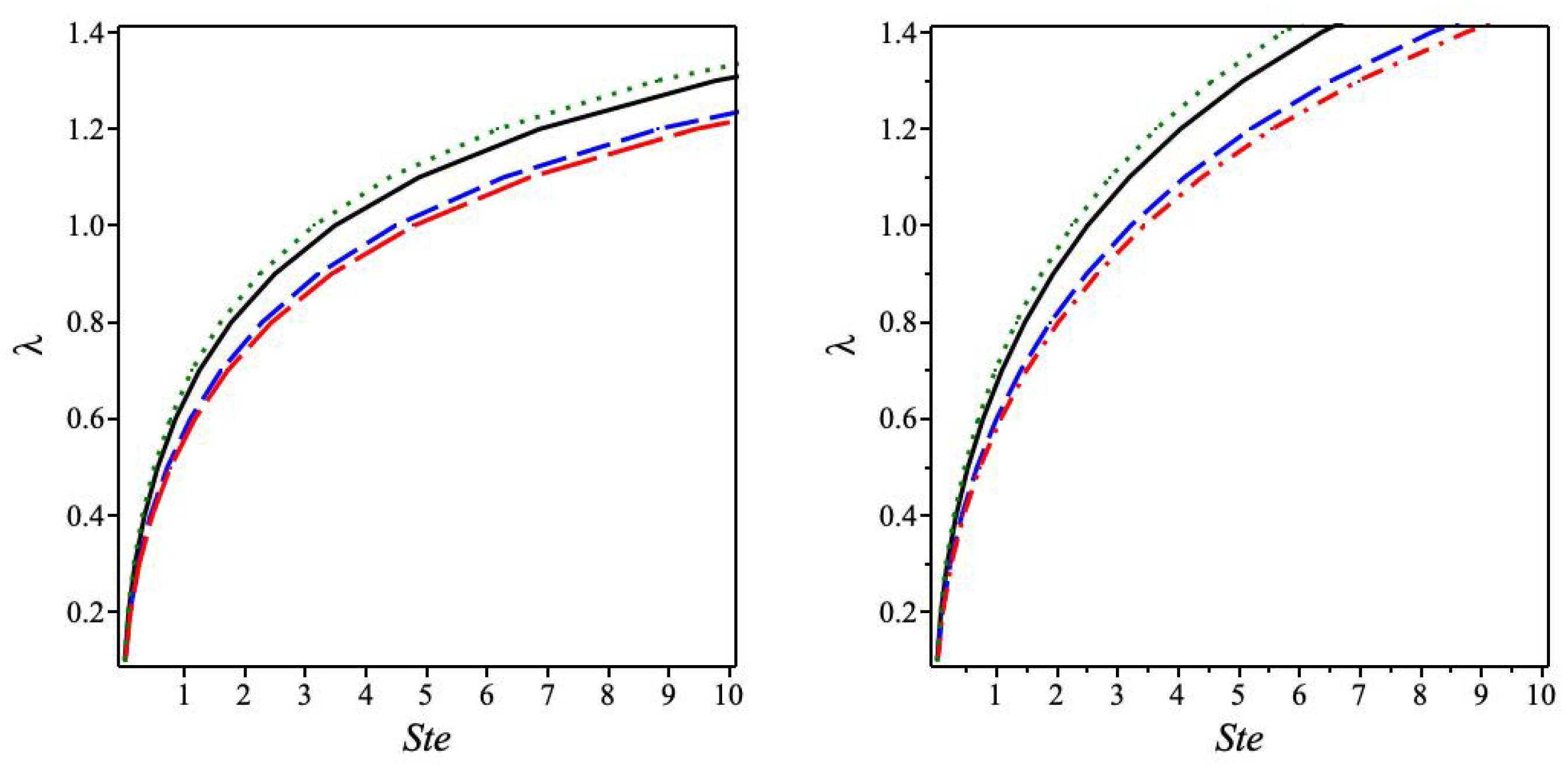
To explore the solutions of the nonlinear Equation (28), we present in Figure 1 the variation of λ in terms of the Stefan constant S t e following Equation (28) for δ 1 = δ 2 = 1 (left panel), δ 1 = δ 2 = 5 (right panel), and various values of p = 0.5 , 1 , 1.5 , 2.5 . It is obvious that a small value of Stefan’s constant S t e allows for the achievement of the boundary condition λ = 1 , for the case δ 1 = δ 2 = 5 .

3.2. Case 2: Ψ 1 ( x ) Ψ 2 ( x )

From (25) and Ψ 2 Ψ 1 1 + δ 2 , x [ 0 , λ ] , we have
2 λ S t e = 4 S t e e ( 1 + δ 2 ) λ 2 0 λ e ( 1 + δ 2 ) ξ 2 β ( ξ ) d ξ + K 1 e ( 1 + δ 2 ) λ 2 .
Substituting the expression of K 1 into (29), we obtain the nonlinear equation of λ , which corresponds to the first approximation y 1 .
λ π 1 + δ 2 erf ( λ 1 + δ 2 ) + 4 e ( 1 + δ 2 ) λ 2 π 2 1 + δ 2 erf ( λ 1 + δ 2 ) 1 0 λ e ( 1 + δ 2 ) x 2 β ( x ) d x ( 1 + δ 1 p + 1 ) e ( 1 + δ 2 ) λ 2 S t e = 0 .
With the appropriate choice of the function β ( x ) = 1 2 e ( 1 + δ 2 ) x 2 , we get the transcendental equation
erf ( λ 1 + δ 2 ) λ 1 + δ 2 ( e ( 1 + δ 2 ) λ 2 + 1 ) π + ( e ( 1 + δ 2 ) λ 2 1 ) = ( 1 + δ 2 ) ( 1 + δ 1 p + 1 ) S t e .
Similarly, from (25) and Ψ 2 Ψ 1 1 1 + δ 1 , x [ 0 , λ ] , we have
2 λ S t e = 4 S t e e λ 2 1 + δ 1 0 λ e ξ 2 1 + δ 1 β ( ξ ) d ξ + K 2 e λ 2 1 + δ 1 .
Substituting the value of K 2 into (43), we obtain the nonlinear equation of λ , which corresponds to the second approximation y 2
λ π 1 + δ 1 erf ( λ 1 + δ 2 ) + 4 e λ 2 1 + δ 1 π 1 + δ 1 2 erf ( λ 1 + δ 1 ) 1 0 λ e ( 1 + δ 1 ) x 2 β ( x ) d x ( 1 + δ 1 p + 1 ) e λ 2 1 + δ 1 S k e = 0 .
With the appropriate choice of the function β ( x ) = 1 2 e x 2 1 + δ 1 , we get the transcendental equation
λ π 1 + δ 1 erf ( λ 1 + δ 1 ) ( e λ 2 1 + δ 1 + 1 ) + ( δ 1 + 1 ) ( e λ 2 1 + δ 1 1 ) = ( 1 + δ 1 p + 1 ) S t e
Thus, we have deduced the approximate solutions of BVP (1) and (2) in implicit forms.
Lemma 3
If Ψ 1 ( x ) Ψ 2 ( x ) and ( y , λ ) is a solution of BVP (1) and (2), then the first approximate solution y 1 is given by (16) and (17), and λ satisfies the corresponding nonlinear algebraic Equation (30).
and
Lemma 4
If Ψ 1 ( x ) Ψ 2 ( x ) and ( y , λ ) is a solution of BVP (1) and (2), then the second approximate solution y 2 is given by (21) and (22), and λ satisfies the corresponding nonlinear algebraic Equation (33).
To investigate the solutions of the nonlinear Equations (31) and (34), we show in Figure 2 the change of λ in terms of the Stefan constant S t e , using Equations (31) (left panel) and (34) (right panel), for δ 1 = 1 , δ 2 = 0.1 as well as a range of p = 0.5 , 1 , 5 , 10 . Obviously, the boundary value λ = 1 for the first instance necessitates a large value of Stefan’s constant S t e , but the boundary value for the second case may be achieved with a modest value of S t e . The boundary requirement λ = 1 is also satisfied in the second case for modest values of Stefan’s constant S t e , whereas the first example needed huge values of S t e .

4. Remarks on the General Case: δ 1 > 1 and δ 2 0

It is useful to consider the general case with δ 1 > 1 and δ 2 > 0 before addressing the numerical discussion of the proposed approximations. Based on the previous procedure, we obtain
1 Ψ 2 Ψ 1 1 + δ 2 1 + δ 1 , δ 1 > 1 a n d δ 2 0 .
For
Ψ 2 Ψ 1 1 + δ 2 1 + δ 1 , x [ 0 , λ ] .
With a simple substitution of this into (3) and (8), we obtain the first approximate solution to BVP (1):
y 1 , δ i + δ 1 p + 1 y 1 , δ i p + 1 = 1 + δ 1 p + 1 + 4 S t e 0 x e 1 + δ 2 1 + δ 1 η 2 0 η e 1 + δ 2 1 + δ 1 ξ 2 β ( ξ ) d ξ d η + K 1 , δ i 0 x e 1 + δ 2 1 + δ 1 η 2 d η ,
where
K 1 , δ i = 1 + δ 1 p + 1 + 4 S t e 0 λ e 1 + δ 2 1 + δ 1 x 2 0 x β ( ξ ) e 1 + δ 2 1 + δ 1 ξ 2 d ξ d x 0 λ e 1 + δ 2 1 + δ 1 x 2 d x .
By using this case and repeating the above calculations, we can obtain λ in terms of S t e . Thus,
2 λ S t e = 4 S t e e 1 + δ 2 1 + δ 1 λ 2 0 λ e 1 + δ 2 1 + δ 1 ξ 2 β ( ξ ) d ξ + K 1 , δ i e 1 + δ 2 1 + δ 1 λ 2 .
Similarly, for
Ψ 2 Ψ 1 1 , x [ 0 , λ ] ,
with a simple substitution of this into (3) and (8), we obtain the second approximate solution to BVP (1), as follows:
y 2 , δ i + δ 1 p + 1 y 2 , δ i p + 1 = 1 + δ 1 p + 1 + 4 S t e 0 x e η 2 0 η e ξ 2 β ( ξ ) d ξ d η + K 2 , δ i 0 x e η 2 d η ,
where
K 2 , δ i = 1 + δ 1 p + 1 + 4 S t e 0 λ e x 2 0 x β ( ξ ) e ξ 2 d ξ d x 0 λ e x 2 d x ,
and the values of λ in terms of the Stefan number S t e are given by
2 λ S t e = 4 S t e e λ 2 0 λ e ξ 2 β ( ξ ) d ξ + K 2 , δ i e λ 2 .
In these cases, the proof is almost identical to that in the above cases when δ i 0 , i = 1 , 2 .

5. Discussion

For numerical validation, we utilized the Maple software, which is a powerful tool offering advanced numerical techniques. Additionally, we created a user-friendly program with simple statements to solve boundary value problems (BVP) using this software. The program automatically detects the type of problem and selects an appropriate algorithm. In our case, the middefer method was employed, which is a midpoint method that incorporates enhancement schemes. The Richardson extrapolation method is typically faster for enhancement schemes, while deferred corrections use less memory for challenging problems. Furthermore, this method can handle harmless end-point singularities that the trapezoidal scheme cannot. The numerical technique also employs a beneficial strategy using the continuation method, which modifies the coefficient of the second-order derivative of the equation. This method reduces the global error by selecting an appropriate number of maxmesh [30].
To begin with, it is interesting to explore whether the prior results numerically satisfy the requirement y ( λ ) = 2 λ S t e , which is associated with the system (1). We will restrict our investigation to the δ 1 = δ 2 case.
In Table 1, we present a comparison between the numerical value of the first derivative y ( λ ) of Equation (2) and the value 2 λ / S t e obtained from Equation (28). It is clear that for a modestly large values of p, the two results are in good agreement with our approximation at this stage.
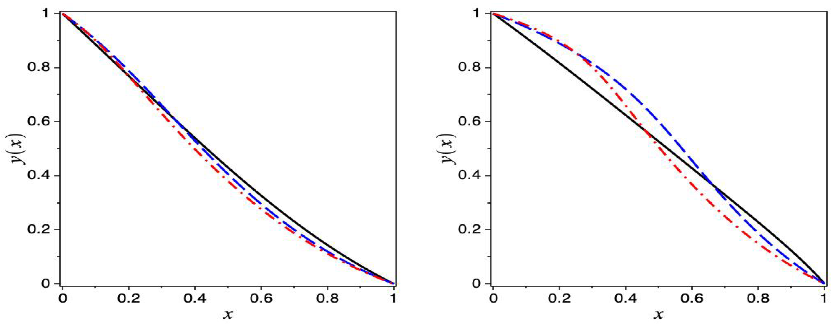
In Figure 3, we present the numerical solution in terms of the independent variable x for two cases, δ 1 = δ 2 = 1 (left panel) and δ 1 = δ 2 = 5 (right panel), and for different values of p = 1 , 5 , 10 .
In Figure 4, we present the analytical solution in the implicit form given by Equation (23) in terms of the independent variable x for two cases, δ 1 = δ 2 = 1 (left panel) and δ 1 = δ 2 = 5 (right panel), and for different values of p = 1 , 5 , 10 . The obtained results show good agreement between the analytical solution in the implicit form given by Equation (23) and the numerical solution when the nonlinear approximated equation given by Equation (28) is used for the case δ 1 = δ 2 .
The numerical values for the situation δ 1 = δ 2 = 5 and various values of the parameter p = 1 , 5 , 10 are included in Table 2 to allow for a more detailed comparison of the numerical solution of BVP (1) with the analytical solution in implicit form given by Equation (23). It is well-established and prevalent that these ideals perfectly coincide. They make our proposed approximation more acceptable in the situation of δ 1 = δ 2 and, with this approximation in hand, will provide instruments to study more complex physical cases.
In Table 3, we present a comparison between the value of the numerical first derivation y ( λ ) of Equation (2) and the value 2 λ / S t e obtained from Equation (31) for δ 1 = 1 , δ 2 = 0.1 . It is clear that, for large values of p, the two values are in good agreement. Thus, the suggested approximation shows that the condition y ( λ ) = 2 λ S t e is well satisfied for λ > 0 in the case δ 1 δ 2 and large values of p .
In Figure 5, we present the numerical solutions y ( x ) of BVP (1) in terms of the independent variable x (left panel) and the first approximation y 1 ( x ) given by Equation (16) (right panel). Both cases are for δ 1 = 1 , δ 2 = 0.1 , and for different values of p = 1 , 5 , 10 . The obtained results show good agreement between the first approximation in Equation (16) and the numerical solution when the nonlinear approximated Equation (31) is used for the case δ 1 δ 2 .
To further illustrate the comparison between the numerical solution and the first approximation solution, we present the numerical values in Table 4 for the case δ 1 = 1 , δ 2 = 0.1 and different values of p = 1 , 5 , 10 . Good agreement is present between both solutions.
Now, we can explore numerically the second approximation in Equation (21) of the BVP (1) with the boundary λ = 1 for the case δ 1 δ 2 . We present in Table 5 a comparison between the numerical values of BVP (1) and the second approximation in Equation (21) for an appropriate choice of the function, β ( x ) = 1 2 e x 2 1 + δ 1 , with δ 1 = 0.1 , δ 2 = 1 , and different values of p = 1 , 5 , 10 . It turns out that the second approximate values are in good agreement with the numerical values. On the other hand, the choice of the values for the parameters δ 1 and δ 2 is guided by the satisfaction of the condition y ( λ ) = 2 λ S t e .

6. Conclusions

We have discussed the conceptual model, which is more precise, realistic, and practical for actual applications, that arises from the phase-change Stefan issue with variable thermal coefficients. This proposed model has two approximately appropriate solutions. Finding the explicit forms of the solutions in specific circumstances allows for the determination of the associated thermal coefficients of thermal conductivity. It is extensively discussed in a fascinating scenario where the thermal coefficient is higher than −1.
Exceptional approximations are provided, and the obtained results are in good agreement with those obtained numerically. We predict that the approximation solutions we have proposed will be useful in investigating more useful heat transfer processes that can be governed by the one-phase Stefan equation with variable thermal coefficients of a high order.

Author Contributions

Conceptualization, L.B., S.B. and A.K.; methodology, L.B., S.B. and A.K.; software, S.B.; validation, L.B., S.B. and A.K.; formal analysis, L.B., S.B. and A.K.; investigation, L.B., S.B. and A.K.; writing—original draft preparation, L.B., S.B. and A.K.; writing—review and editing, L.B., S.B. and A.K. All authors have read and agreed to the published version of the manuscript.

Funding

This research received no external funding.

Institutional Review Board Statement

Hereby we confirm that the article is not under consideration in other journals.

Informed Consent Statement

Not applicable.

Data Availability Statement

Data available on the request through the corresponding author.

Acknowledgments

The authors extend their appreciation to the Deanship of Scientific Research at Imam Mohammad Ibn Saud Islamic University for funding this work through Research Group No. RG-21-09-14.

Conflicts of Interest

The authors declare no conflict of interest.

References

  1. Cho, S.H.; Sunderland, J.E. Phase change problems with temperature-dependent thermal Conductivity. J. Heat Transfer 1974, 96, 214–217. [Google Scholar] [CrossRef]
  2. Oliver, D.L.R.; Sunderland, J.E. A phase-change problem with temperature-dependent thermal conductivity and specific heat. Int. J. Heat Mass Transfer 1987, 30, 2657–2661. [Google Scholar] [CrossRef]
  3. Ceretani, A.N.; Salva, N.N.; Tarzia, D.A. Existence and uniqueness of the modified error function. Appl. Math. Lett. 1987, 70, 14–17. [Google Scholar] [CrossRef]
  4. Bougouffa, S.; Khanfer, A.; Bougoffa, L. On the approximation of the modified error function. Math. Meth. Appl. Sci. 2022, 1–9. [Google Scholar] [CrossRef]
  5. Khanfer, A.; Bougoffa, L. A Stefan problem with nonlinear thermal conductivity. Math. Meth. Appl. Sci. 2022, 1–10. [Google Scholar] [CrossRef]
  6. Bollati, J.; Natale, M.F.; Semitiel, J.A.; Tarzia, D.A. Exact solution for non-classical one-phase Stefan problem with variable thermal coefficients and two different heat source terms. Comp. Appl. Math. 2022, 41, 375. [Google Scholar] [CrossRef]
  7. Briozzo, A.C.; Tarzia, D.A. Existence, Uniqueness and an Explicit Solution for a One-Phase Stefan Problem for a Non-Classical Heat Equation, Free Boundary Problems; International Series of Numerical Mathematics; Birkhäuser: Basel, Switzerland, 2006; Volume 15, pp. 117–124. [Google Scholar]
  8. Bougoffa, L. A note on the existence and uniqueness solutions of the modified error function. Math. Methods Appl. Sci. 2018, 41, 5526–5534. [Google Scholar] [CrossRef]
  9. Bougoffa, L.; Rach, R.; Mennouni, A. On the existence, uniqueness and new analytic approximate solution of the modified error function in two-phase Stefan problems. Math. Methods Appl. Sci. 2021, 44, 10948–10956. [Google Scholar] [CrossRef]
  10. Zhou, Y.; Xia, L. Exact solution for Stefan problem with general power-type latent heat using Kummer function. Int. J. Heat Mass Transf. 2015, 84, 114–118. [Google Scholar] [CrossRef]
  11. Kumar, A.; Singh, A.K. A moving boundary problem with variable specific heat and thermal conductivity. J. King Saud Univ.-Sci. 2020, 32, 384–389. [Google Scholar] [CrossRef]
  12. Ribera, H.; Myers, T. A mathematical model for nanoparticle melting with size-dependent latent heat and melt temperature. Microfluid. Nanofluidics 2016, 20, 147. [Google Scholar] [CrossRef]
  13. Font, F.; Myers, T.; Mitchell, S. A mathematical model for nanoparticle melting with density change. Microfluid. Nanofluidics 2015, 18, 233–243. [Google Scholar] [CrossRef]
  14. Briozzo, A.C.; Natale, M.F. One-phase Stefan problem with temperature-dependent thermal conductivity and a boundary condition of Robin type. J. Appl. Anal. 2015, 21, 89–97. [Google Scholar] [CrossRef]
  15. Bougoffa, L.; Khanfer, A. On the solutions of a phase change problem with temperature-dependent thermal conductivity and specific heat. Results Phys. 2020, 19, 103646. [Google Scholar] [CrossRef]
  16. Voller, V.R.; Swenson, J.B.; Paola, C. An analytical solution for a Stefan problem with variable latent heat. Int. J. Heat Mass Transf. 2004, 47, 5387–5390. [Google Scholar] [CrossRef]
  17. Beasley, J.D. Thermal conductivities of some novel nonlinear optical materials. Appl. Opt. 1994, 33, 1000–1003. [Google Scholar] [CrossRef]
  18. Aggarwal, R.L.; Fan, T.V. Thermal diffusivity, specific heat, thermal conductivity, coefficient of thermal expansion, and refractive-index change with temperature in AgGaSe_2. Appl. Opt. 2005, 44, 2673. [Google Scholar] [CrossRef]
  19. Henager, C.H.; Pawlewicz, W.T. Thermal conductivities of thin, sputtered optical films. Appl. Opt. 1993, 32, 91. [Google Scholar] [CrossRef]
  20. de Azevedo, A.M.; dos Santos Magalhães, E.; da Silva, R.G.D. A comparison between nonlinear and constant thermal properties approaches to estimate the temperature in LASER welding simulation. Case Stud. Therm. Eng. 2022, 35, 102135. [Google Scholar] [CrossRef]
  21. Xiao, Y.; Wu, H. An explicit coupled method of FEM and meshless particle method for simulating transient heat transfer process of friction stir welding. Math. Probl. Eng. 2020, 2020, 2574127. [Google Scholar] [CrossRef]
  22. Brizes, E.; Jaskowiak, J.; Abke, T.; Ghassemi-Armaki, H.; Ramirez, A.J. Evaluation of heat transfer within numerical models of resistance spot welding using high-speed thermography. J. Mater. Process. Technol. 2021, 297, 117276. [Google Scholar] [CrossRef]
  23. Gladkov, S.O.; Bogdanova, S.B. On the Theory of Nonlinear Thermal Conductivity. Tech. Phys. 2016, 61, 157–164. [Google Scholar] [CrossRef]
  24. Tomeczek, J.; Palugniok, H. Specific heat capacity and enthalpy of coal pyrolysis at elevated temperatures. Fuel 1996, 75, 1089–1093. [Google Scholar] [CrossRef]
  25. Saxena, S.K. Earth mineralogical model: Gibbs free energy minimization computation in the system MgO–FeO–SiO2. Geochim. Cosmochim. Acta 1996, 60, 2379–2395. [Google Scholar] [CrossRef]
  26. Hanrot, F.; Ablitzer, D.; Houzelot, J.L.; Dir, M. Experimental measurement of the true specific heat capacity of coal and semicoke during carbonization. Fuel 1994, 73, 305–309. [Google Scholar] [CrossRef]
  27. Haemmerich, D.; Dos Santos, I.; Schutt, D.J.; Webster, J.G.; Mahvi, D.M. In vitro measurements of temperature-dependent specific heat of liver tissue. Med. Eng. Phys. 2006, 28, 194–197. [Google Scholar] [CrossRef]
  28. Alam, M.N.; Tunç, C. New solitary wave structures to the (2+1)-dimensional KD and KP equations with spatiotemporal dispersion. J. King Saud Univ.-Sci. 2020, 32, 3400–3409. [Google Scholar] [CrossRef]
  29. Akinshilo, A.T.; Davodi, A.G.; Rezazadeh, H.; Sobamowoand, G.; Tunç, C. Heat transfer and flow of MHD micropolar nanofluid through the porous walls, magnetic fields, and thermal radiation. Palest. J. Math. 2022, 11, 604–616. [Google Scholar]
  30. Ascher, U.; Petzold, L. Computer Methods for Ordinary Differential Equations and Differential-Algebraic Equations; SIAM: Philadelphia, PA, USA, 1998. [Google Scholar]
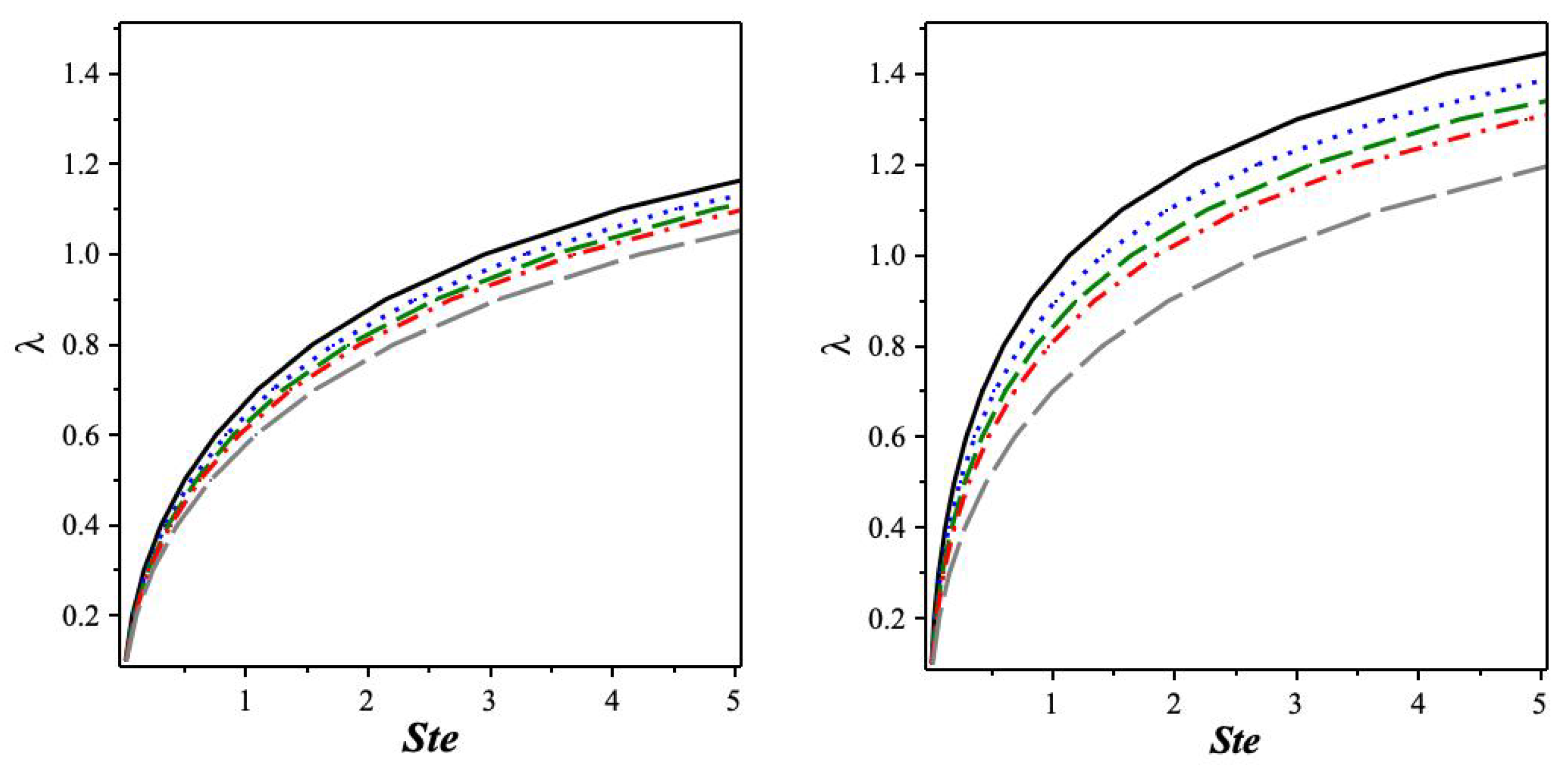
Figure 1. The variation of λ , in terms of the Stefan constant S t e , from Equation (28). For δ 1 = δ 2 = 1 (left panel), δ 1 = δ 2 = 5 (right panel), different values of p = 0.5 , 1 , 1.5 , 2.5 from the highest line to the lowest, respectively.
Axioms 12 00497 g001
Figure 2. The variation of λ , in terms of the Stefan constant S t e , from Equations (31) and (34). (Left panel) from Equation (31), (right panel) from Equation (34), for δ 1 = 1 , δ 2 = 0.1 , and different values of p = 0.5 , 1 , 5 , 10 from the highest line to the lowest, respectively.
Axioms 12 00497 g002
Figure 3. The numerical solution for the boundary λ = 1 for different values of p. (Left panel) δ 1 = δ 2 = 1 , (right panel) δ 1 = δ 2 = 5 . Solid black line: p = 1 , dashed blue line: p = 5 , and dashed–dotted red line: p = 10 .
Axioms 12 00497 g003
Figure 4. The analytical solution in implicit form given by Equation (23) for the boundary λ = 1 for different values of p. (Left panel) δ 1 = δ 2 = 1 , (right panel) δ 1 = δ 2 = 5 . Solid black line: p = 1 , dashed blue line: p = 5 , and dashed–dotted red line: p = 10 .
Axioms 12 00497 g004
Figure 5. Comparison between the numerical solutions of BVP (1) and the first approximation in Equation (16) for the boundary λ = 1 , for different values of p. The (left panel) represents the numerical solutions, while the (right panel) represents the first approximation as in Equation (16). In both cases δ 1 = 1 , δ 2 = 0.1 , solid black line: p = 1 , dashed blue line: p = 5 , and dashed–dotted red line: p = 10 . For the function, β ( x ) = 1 2 e ( 1 + δ 2 ) x 2 .
Axioms 12 00497 g005
Table 1. Comparison between the numerical value of the first derivative y ( λ ) and analytic expression ( 2 λ / S t e ) from Equation (28) for the case δ 1 = δ 2 = 1 .
p0.10.511.52510
2 λ / S t e −0.7758−0.6773−0.6096−0.5689−0.5418−0.4741−0.4433
y ( λ ) −0.4972−0.6441−0.6102−0.5698−0.5427−0.4760−0.4433
Table 2. Comparison between the numerical solution y n u m of BVP (1) for the boundary λ = 1 and the analytical approximation y a p p given by Equation (23) for δ 1 = δ 2 = 5 and for different values of p = 1 , 5 , 10 . For the function, β ( x ) , see the text.
p = 1 p = 5 p = 10
x y app y num y app y num y app y num
01.000001.000001.000001.000001.000001.00000
0.10.9099600.9099040.9496650.9496180.9572710.957223
0.20.8166900.8165900.8892240.8891940.8962050.896159
0.30.7210900.7208600.8147920.8147630.8005570.800429
0.40.6239840.6236940.7203190.7202190.6592030.659085
0.50.5260440.5257060.5993100.5990760.5058680.505774
0.60.4276540.4271910.4560120.4559110.3677320.367636
0.70.3286950.3282490.3128720.3128590.2488490.248768
0.80.2280780.2275400.1875510.1875080.1488300.148778
0.90.1224160.1224370.08374420.08371480.06644190.0664179
1.0 4 × 10 6 0.000000.000000.000000.000000.00000
Table 3. Comparison between the numerical value of the first derivative y ( λ ) and analytic expression ( 2 λ / S t e ) from Equation (31) for δ 1 = 1 , δ 2 = 0.1 .
p0.10.511.52510
2 λ / S t e −0.7310−0.6382−0.5740−0.5360−0.5102−0.4468−0.4178
y ( λ ) −0.6851−0.8026−0.7092−0.6315−0.5855−0.4897−0.4539
Table 4. Comparison between the numerical solution y n u m of BVP (1) for the boundary λ = 1 and the first approximation y 1 Equation (16) for δ 1 = 1 , δ 2 = 0.1 and for different values of p = 1 , 5 , 10 . For the function, β ( x ) = 1 2 e ( 1 + δ 2 ) x 2 .
p = 1 p = 5 p = 10
x y 1 y num y 1 y num y 1 y num
01.000001.000001.000001.000001.000001.00000
0.10.883530.8943050.9013840.9059880.8984490.902000
0.20.765330.7856590.7842700.7937800.7648440.772572
0.30.647520.6763220.6536880.6675040.6229020.633430
0.40.532290.5675230.5208630.5368250.4901170.501984
0.50.421780.4600920.3965900.4125530.3714420.383526
0.60.318020.3554520.2865880.3009620.2680650.279297
0.70.222770.2555410.1925620.2042560.1800660.189469
0.80.137460.1615060.1142700.1224980.1068510.113620
0.90.063060.07535240.0506000.0548360.04731410.0508684
1.0 8 × 10 6 0.000000.0000130.000000.000000.00000
Table 5. Comparison between the numerical solution y n u m of BVP (1) for the boundary λ = 1 and the second approximation y 2 of Equation (21) for δ 1 = 0.1 , δ 2 = 1 and for different values of p = 1 , 5 , 10 . For the function, β ( x ) = 1 2 e x 2 1 + δ 1 .
p = 1 p = 5 p = 10
x y 2 y num y 2 y num y 2 y num
01.00001.000001.000001.000001.000001.00000
0.10.8591280.8448840.8608070.8558190.8594060.855716
0.20.7230920.6968540.7230680.7143100.7198000.713261
0.30.5942570.5599260.5917720.5807420.5880460.579486
0.40.4746240.4367560.4702820.4582810.4669550.457202
0.50.3657370.3286850.3605650.3486770.3579140.347866
0.60.2686110.2359520.2635710.2527390.2616130.252179
0.70.1837260.1579800.1795270.1705700.1781900.170217
0.80.1110450.0936450.1081170.1017100.1073110.101518
0.90.0500850.0415100.04861590.04525480.04825360.0451840
1.00.000000.000000.000000.000000.000000.00000
Disclaimer/Publisher’s Note: The statements, opinions and data contained in all publications are solely those of the individual author(s) and contributor(s) and not of MDPI and/or the editor(s). MDPI and/or the editor(s) disclaim responsibility for any injury to people or property resulting from any ideas, methods, instructions or products referred to in the content.