

A New Extension of the Kumaraswamy Exponential Model with Modeling of Food Chain Data
 , ,
, ,  ,
, 
Abstract
1. Introduction
- The new KMKE distribution gives more flexibility than the SEWE model and other well-known statistical models for food chain data as we prove in Section 7.
- The new recommended distribution is quite versatile and comprises three sub-models.
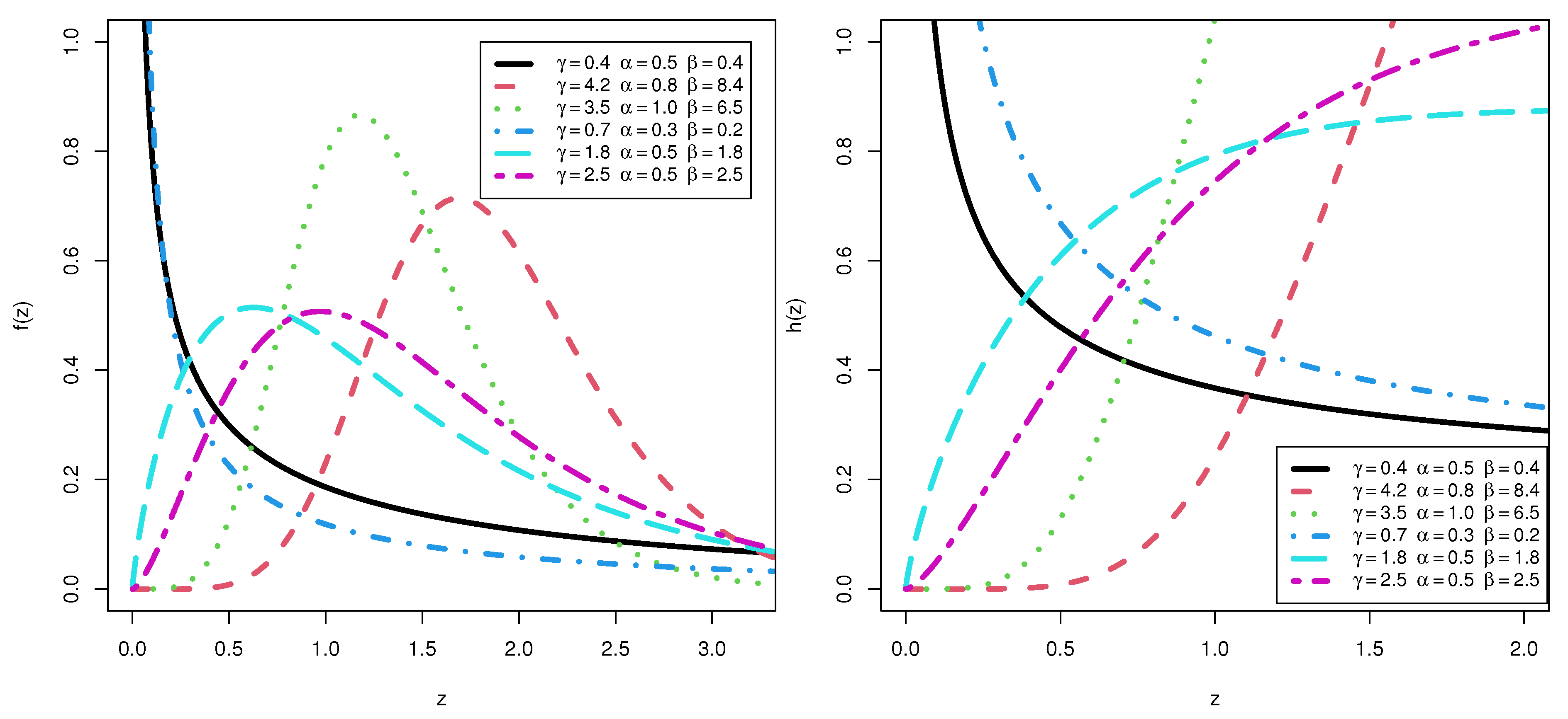
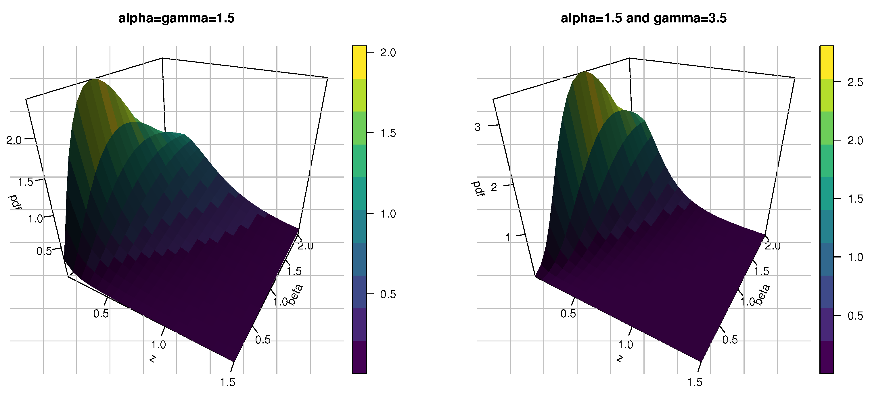
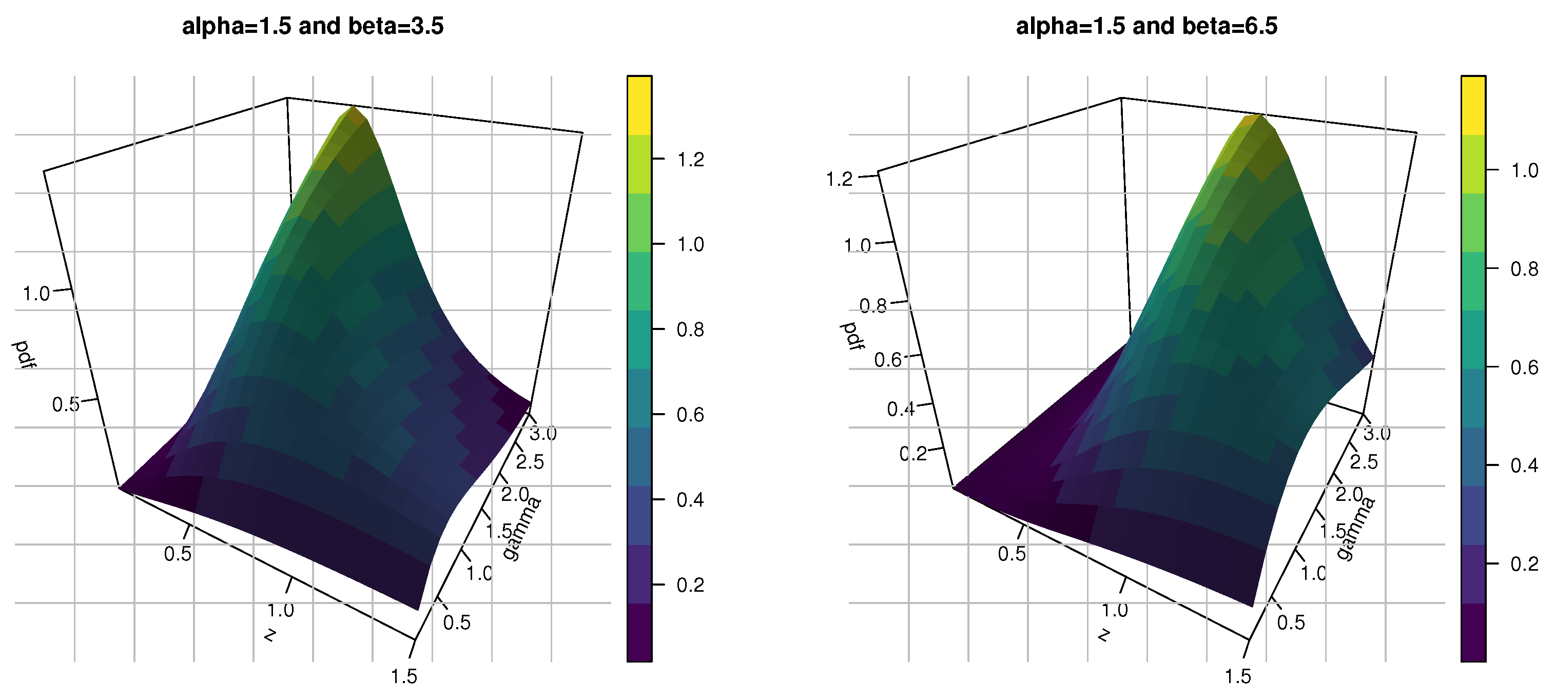
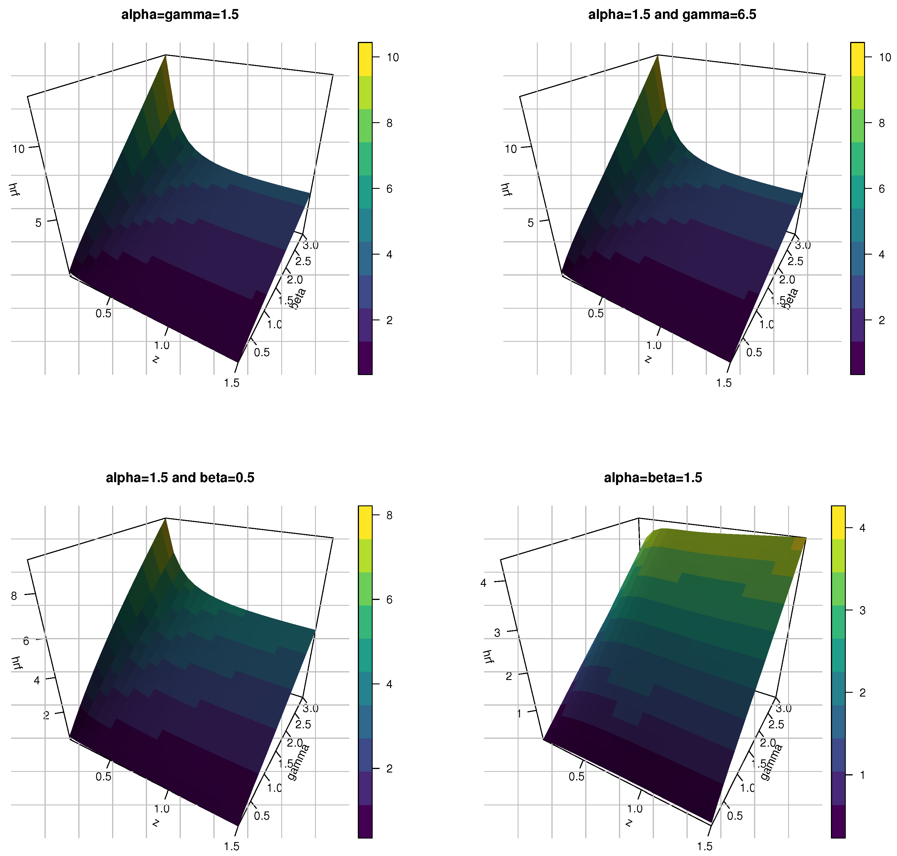
- The shapes of the pdf for the KMKE model can be decreasing, right skewness and uni-modal. However, the hazard rate function (hrf) for the KMKE model can be decreasing, increasing and j-shaped.
- Numerous statistical and computational characteristics of the recently proposed model are investigated.
- The parameters of the KMKE model are estimated utilizing maximum likelihood and Bayesian techniques.
2. Relevant Literature
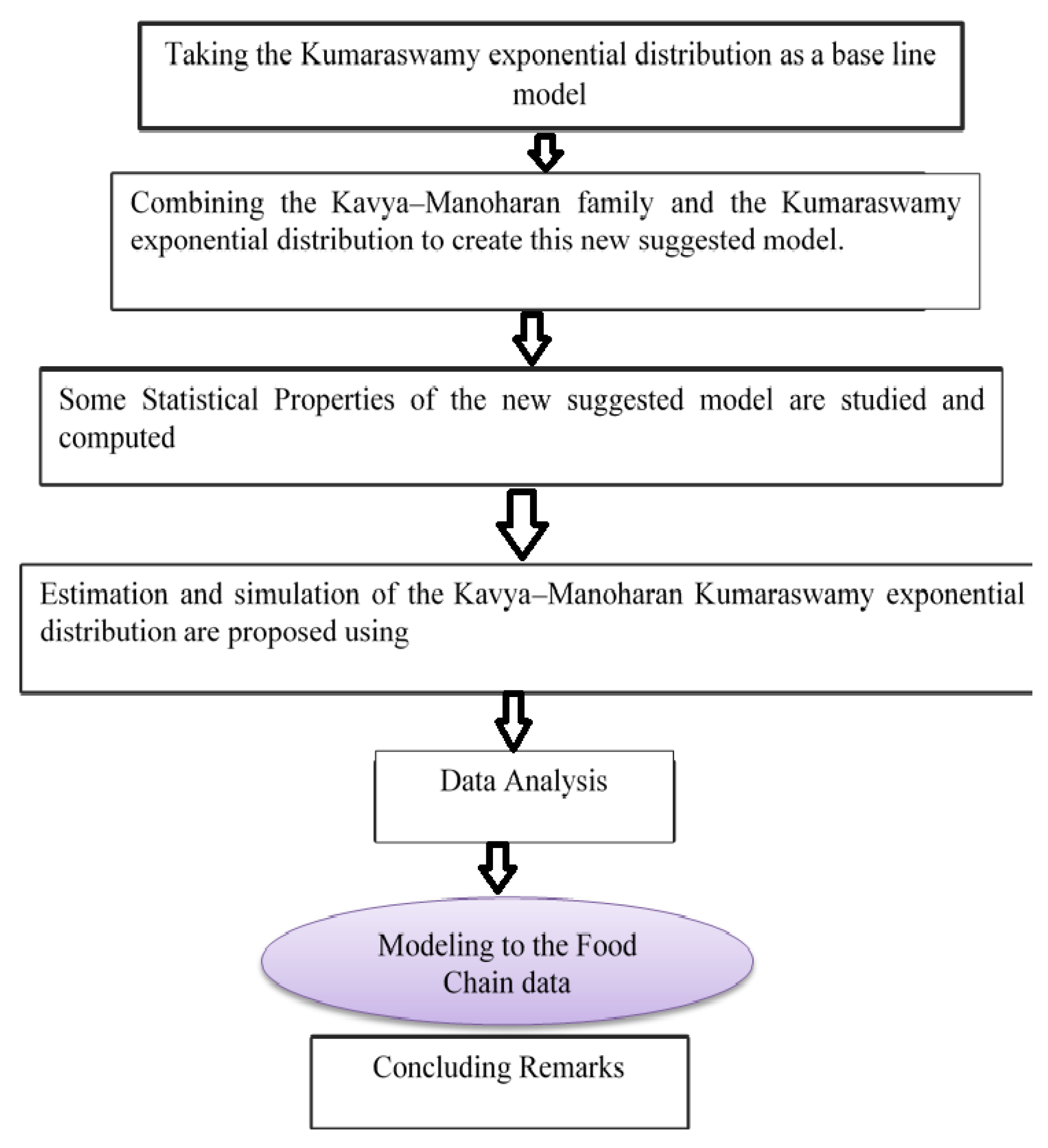
3. The Construction of the Kavya–Manoharan Kumaraswamy Exponential Model
4. Statistical and Computational Features
4.1. Quantile Function
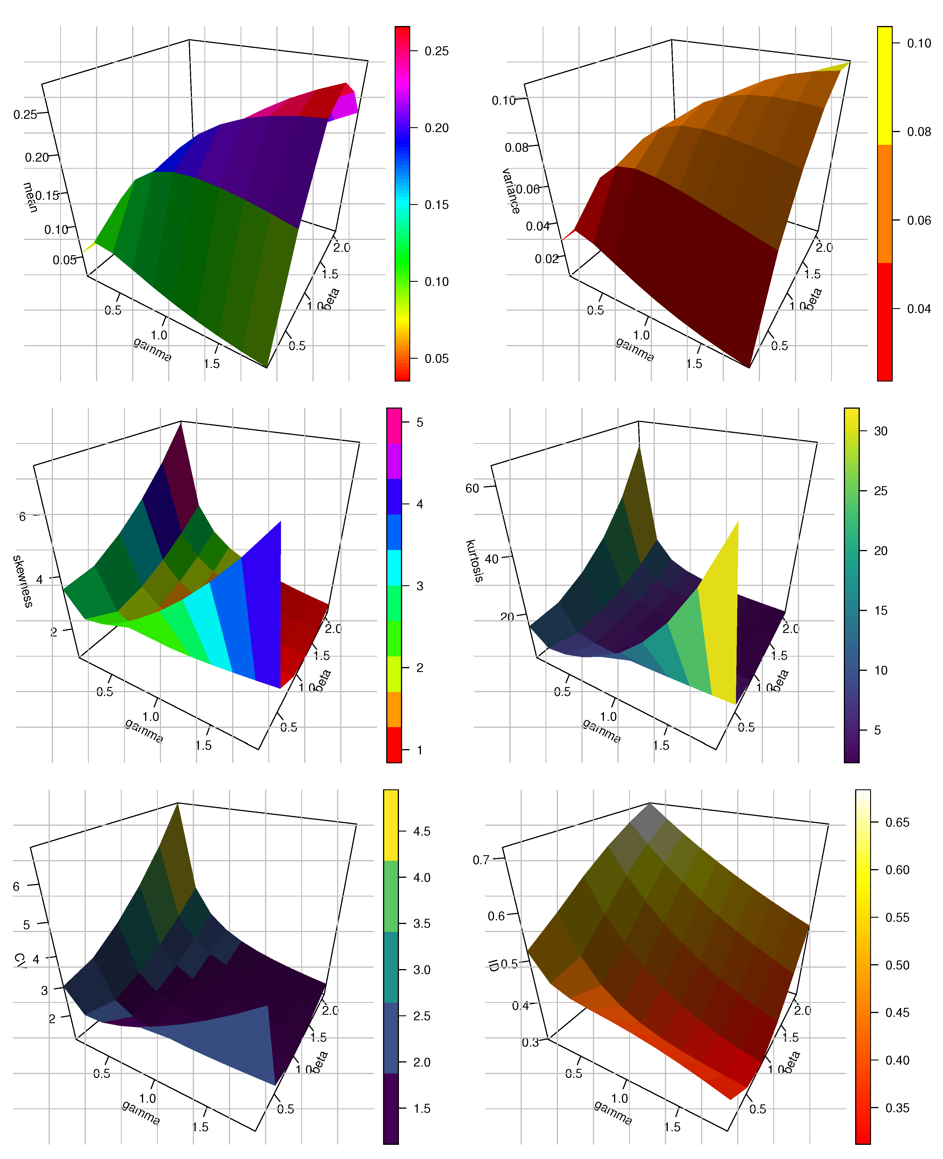
4.2. Moments
5. Estimation Methods
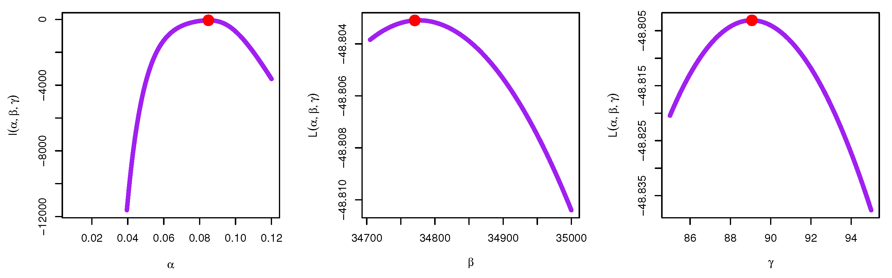
5.1. Maximum Likelihood Estimation
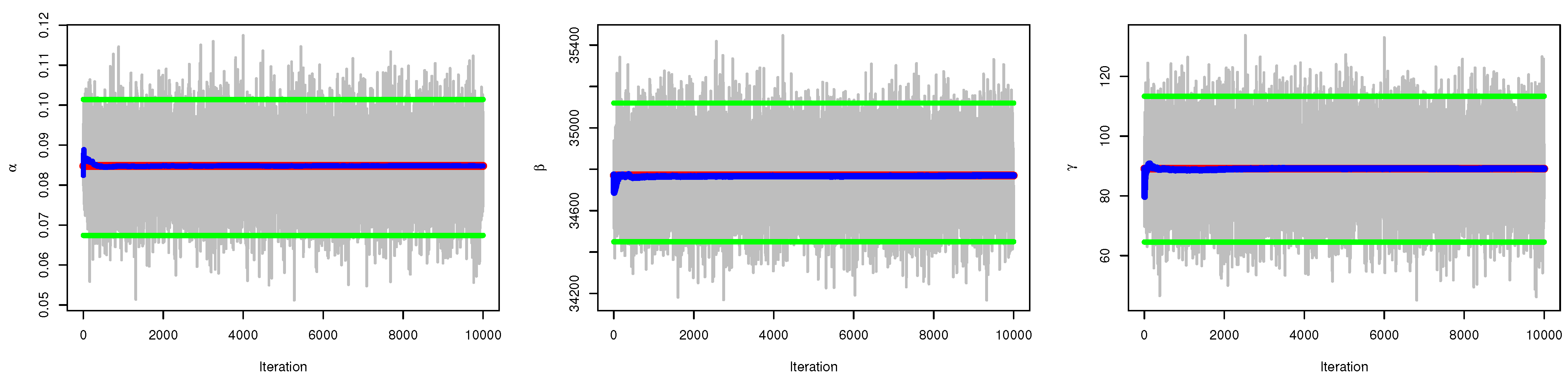
5.2. Bayesian Estimation
6. Simulation
6.1. Simulation Study
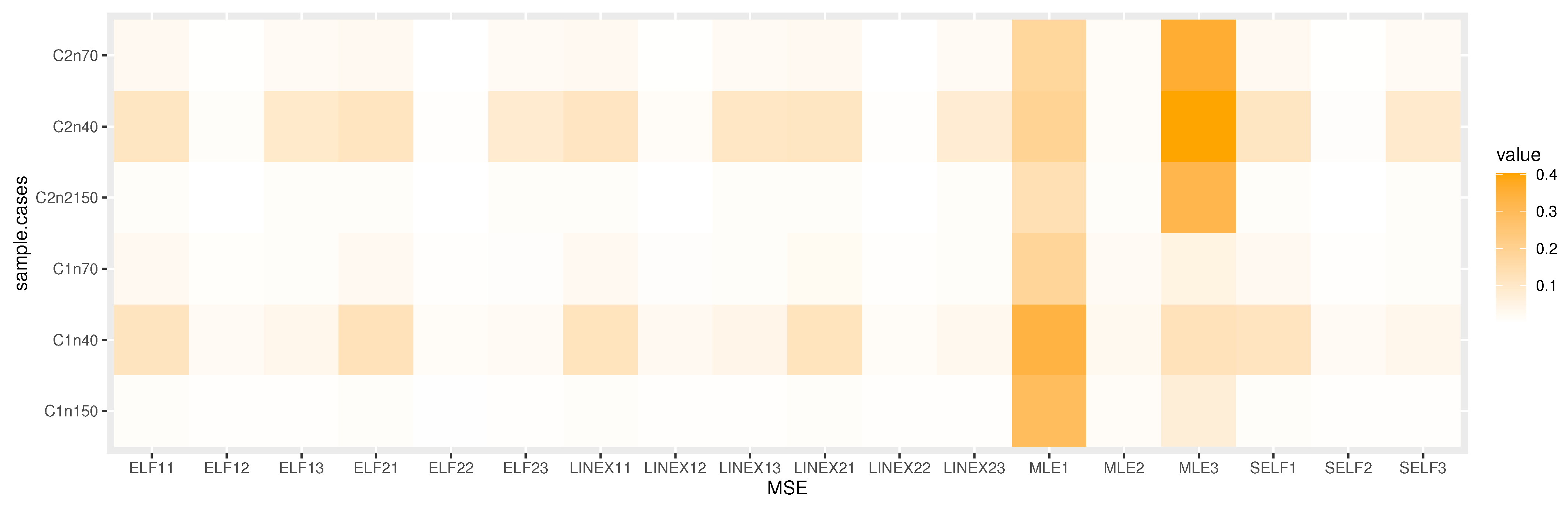
6.2. Final Thoughts on the Simulation Results
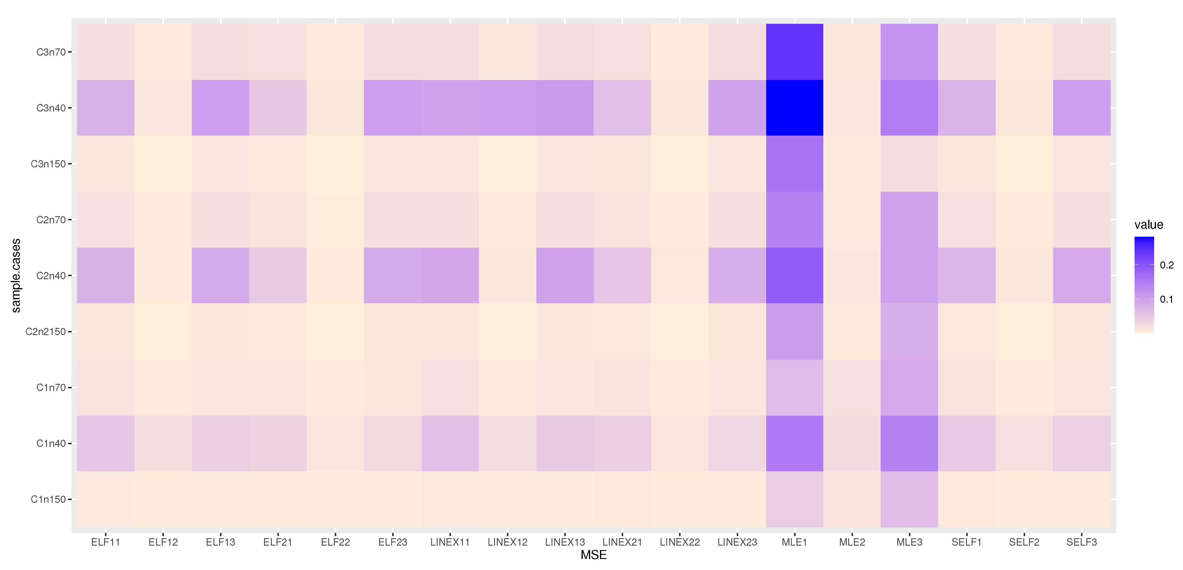
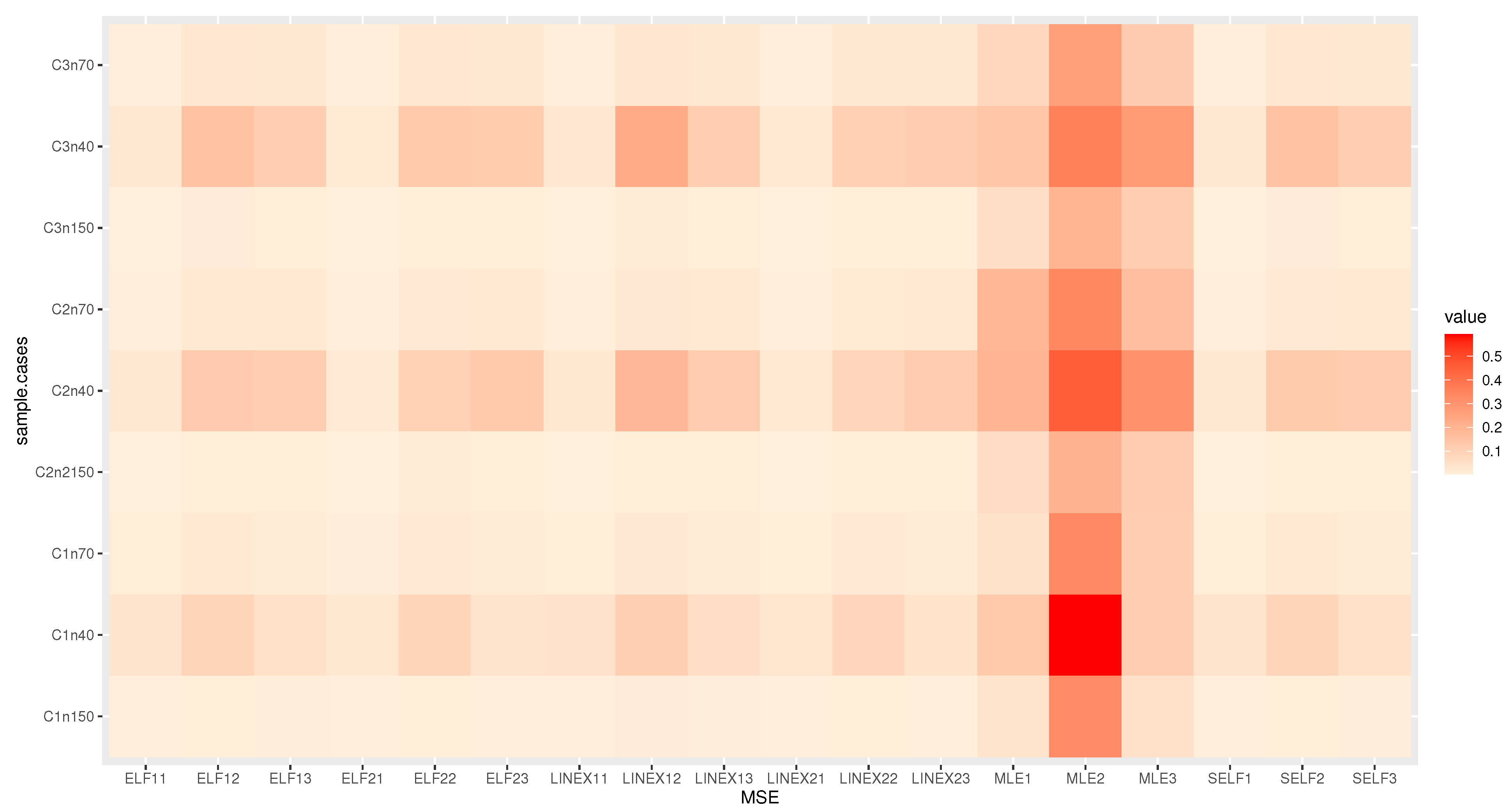
- The Bayesian estimation is superior to the MLE in every situation, we observe.
- The Bayesian estimation with positive weight asymmetric loss function is superior to the Bayesian estimation with negative weight asymmetric loss function, as we note.
- We note that the Bayesian estimation method with positive weight asymmetric loss function is better than the other estimation method.
- The Bayesian estimation with symmetric loss function is superior to the Bayesian estimation with negative weight asymmetric loss function, in some simulations.
- Bayesian credible and HPD intervals are the shortest LCI.
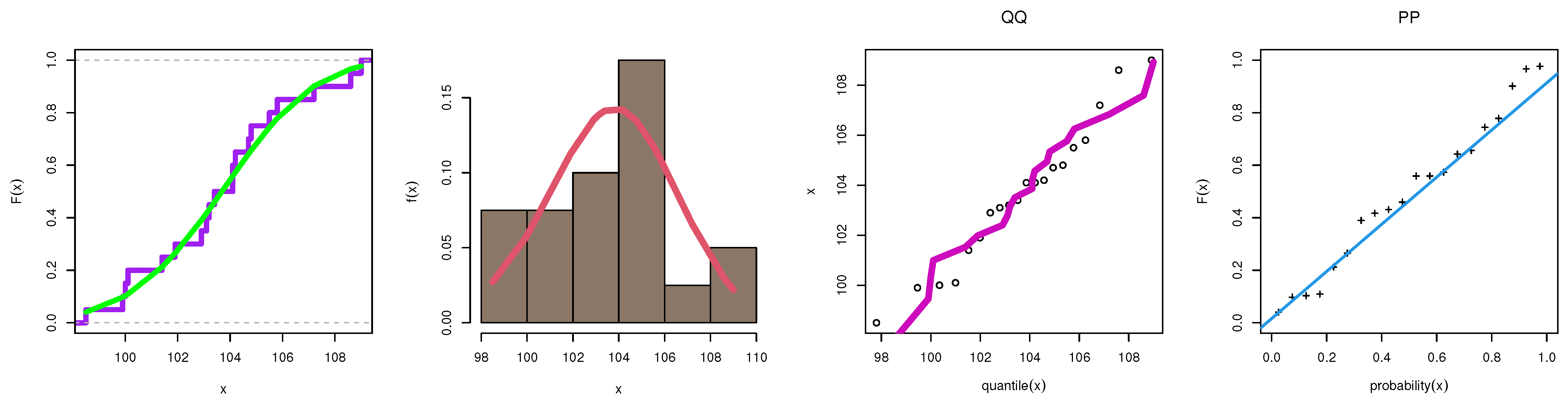
7. Modeling Food Data
8. Concluding Remarks
Author Contributions
Funding
Data Availability Statement
Acknowledgments
Conflicts of Interest
List of Symbols
| Z | Random variable |
| Cumulative distribution function of Kumaraswamy generated family | |
| Cumulative distribution function of exponential distribution | |
| Probability density function of Kumaraswamy exponential distribution | |
| Probability density function of Kumaraswamy exponential distribution | |
| Scale parameter | |
| Shape parameter | |
| Shape parameter | |
| Cumulative distribution function of the Kavya–Manoharan Kumaraswamy exponential distribution | |
| Probability density function of the Kavya–Manoharan Kumaraswamy exponential distribution | |
| Reliability function of the Kavya–Manoharan Kumaraswamy exponential distribution | |
| Hazard rate function of the Kavya–Manoharan Kumaraswamy exponential distribution | |
| Reversed hazard rate function of the Kavya–Manoharan Kumaraswamy exponential distribution | |
| Cumulative hazard rate function of the Kavya–Manoharan Kumaraswamy exponential distribution | |
| Quantile function | |
| The moment | |
| Moment generating function | |
| The incomplete moment | |
| The conditional moment | |
| Log-likelihood function | |
| n | Sample size |
| Shape parameter of hyper-parameter | |
| Scale parameter of hyper-parameter | |
| N | The number of samples |
| Constant of posterior distribution | |
| Squared-error loss function | |
| Bayesian estimator under SELF | |
| Average expectation | |
| LINEX loss function | |
| Bayesian estimator under LINEX | |
| c | Shape parameter of LINEX loss function |
| Entropy loss function | |
| Bayesian estimator under entropy |
Appendix A
References
- Schneider, K.; Hoffmann, I. Nutrition ecology—A concept for systemic nutrition research and integrative problem solving. Ecol. Food Nutr. 2011, 50, 1–17. [Google Scholar] [CrossRef] [PubMed]
- Wezel, A.; Bellon, S.; Doré, T.; Francis, C.; Vallod, D.; David, C. Agroecology as a science, a movement and a practice. A review. Agron. Sustain. Dev. 2009, 29, 503–515. [Google Scholar] [CrossRef]
- Lappé, F.M. Diet for a Small Planet: How to Enjoy a Rich Protein Harvest by Getting Off the Top of the Food Chain. 1971. [Google Scholar]
- Gussow, J.D.; Clancy, K.L. Dietary guidelines for sustainability. J. Nutr. Educ. 1986, 18, 1–5. [Google Scholar] [CrossRef]
- Djekic, I.; Sanjuán, N.; Clemente, G.; Jambrak, A.R.; Djukić-Vuković, A.; Brodnjak, U.V.; Pop, E.; Thomopoulos, R.; Tonda, A. Review on environmental models in the food chain-Current status and future perspectives. J. Clean. Prod. 2018, 176, 1012–1025. [Google Scholar] [CrossRef]
- Almetwally, E.M.; Meraou, M.A. Application of Environmental Data with New Extension of Nadarajah-Haghighi Distribution. Comput. J. Math. Stat. Sci. 2022, 1, 26–41. [Google Scholar] [CrossRef]
- Abubakari, A.G.; Anzagra, L.; Nasiru, S. Chen Burr-Hatke Exponential Distribution: Properties, Regressions and Biomedical Applications. Comput. J. Math. Stat. Sci. 2023, 2, 80–105. [Google Scholar] [CrossRef]
- Marín, S.; Freire, L.; Femenias, A.; Sant’Ana, A.S. Use of predictive modelling as tool for prevention of fungal spoilage at different points of the food chain. Curr. Opin. Food Sci. 2021, 41, 1–7. [Google Scholar] [CrossRef]
- Alyami, S.A.; Elbatal, I.; Alotaibi, N.; Almetwally, E.M.; Elgarhy, M. Modeling to Factor Productivity of the United Kingdom Food Chain: Using a New Lifetime-Generated Family of Distributions. Sustainability 2022, 14, 8942. [Google Scholar] [CrossRef]
- Yu, J.; Chen, H.; Zhang, X.; Cui, X.; Zhao, Z. A Rice Hazards Risk Assessment Method for a Rice Processing Chain Based on a Multidimensional Trapezoidal Cloud Model. Foods 2023, 12, 1203. [Google Scholar] [CrossRef]
- Kumaraswamy, P. A generalized probability density function for double-bounded random processes. J. Hydrol. 1980, 46, 79–88. [Google Scholar] [CrossRef]
- Cordeiro, G.M.; de Castro, M. A new family of generalized distributions. J. Stat. Comput. Simul. 2011, 81, 883–898. [Google Scholar] [CrossRef]
- de Araujo Rodrigues, J.; Madeira Silva, A.P.C. The Exponentiated Kumaraswamy-Exponential Distribution. Curr. J. Appl. Sci. Technol. 2015, 10, 1–12. [Google Scholar] [CrossRef]
- Bakouch, H.; Moala, F.; Saboor, A.; Samad, H. A bivariate Kumaraswamy-exponential distribution with application. Math. Slovaca 2019, 69, 1185–1212. [Google Scholar] [CrossRef]
- Chacko, M.; Mohan, R. Estimation of parameters of Kumaraswamy-Exponential distribution under progressive type-II censoring. J. Stat. Comput. Simul. 2017, 87, 1951–1963. [Google Scholar] [CrossRef]
- Al-saiary, Z.A.; Bakoban, R.A.; Al-zahrani, A.A. Characterizations of the Beta Kumaraswamy Exponential Distribution. Mathematics 2020, 8, 23. [Google Scholar] [CrossRef]
- El-Damrawy, H.H.; Teamah, A.A.M.; El-Shiekh, B.M. Truncated Bivariate Kumaraswamy Exponential Distribution. J. Stat. Appl. Pro. 2022, 11, 461–469. [Google Scholar]
- Chesneau, C.; Jamal, F. The Sine Kumaraswamy-G Family of Distributions. J. Math. Ext. 2021, 15, 1–33. [Google Scholar]
- Hassan, A.S.; Mohamed, R.E.; Kharazmi, O.; Nagy, H.F. A New Four Parameter Extended Exponential Distribution with Statistical Properties and Applications. Pak. J. Stat. Oper. Res. 2022, 18, 179–193. [Google Scholar] [CrossRef]
- Sule, I.; Doguwa, S.; Isah, A.; Jibril, H. The Topp Leone Kumaraswamy-G Family of Distributions with Applications to Cancer Disease Data. JBE 2020, 6, 40–51. [Google Scholar] [CrossRef]
- Arshad, R.M.I.; Tahir, M.H.; Chesneau, C.; Jamal, F. The Gamma Kumaraswamy-G family of distributions: Theory, inference and applications. Stat. Transit. New Ser. 2020, 21, 17–40. [Google Scholar] [CrossRef]
- Afify, A.Z.; Alizadeh, M. The odd Dagum family of distributions: Properties and applications. J. Appl. Probab. Stat. 2020, 15, 45–72. [Google Scholar]
- Tahir, M.H.; Cordeiro, G.M.; Alizadeh, M.; Mansoor, M.; Zubair, M.; Hamedani, G.G. The odd generalized exponential family of distributions with applications. J. Stat. Distrib. Appl. 2015, 2, 1–28. [Google Scholar] [CrossRef]
- Al-Babtain, A.A.; Elbatal, I.; Chesneau, C.; Elgarhy, M. Sine Topp-Leone-G family of distributions: Theory and applications. Open Phys. 2020, 18, 74–593. [Google Scholar] [CrossRef]
- Cordeiro, G.M.; Alizadeh, M.; Ozel, G.; Hosseini, B.; Ortega, E.M.M.; Altun, E. The generalized odd log-logistic class of distributions: Properties, regression models and applications. J. Stat. Comput. Simul. 2017, 87, 908–932. [Google Scholar] [CrossRef]
- Al-Babtain, A.A.; Elbatal, I.; Al-Mofleh, H.; Gemeay, A.M.; Afify, A.Z.; Sarg, A.M. The Flexible BurrX-G Family: Properties, Inference, and Applications in the Engineering Science. Symmetry 2021, 13, 474. [Google Scholar] [CrossRef]
- Alotaibi, N.; Elbatal, I.; Almetwally, E.M.; Alyami, S.A.; Al-Moisheer, A.S.; Elgarhy, M. Truncated Cauchy Power Weibull-G Class of Distributions: Bayesian and Non-Bayesian Inference Modelling for COVID-19 and Carbon Fiber Data. Mathematics 2022, 10, 1565. [Google Scholar] [CrossRef]
- Reyad, H.; Jamal, F.; Othman, S.; Hamedani, G.G. The transmuted Gompertz-G family of distribu-tions: Properties and applications. Tbil. Math. J. 2018, 11, 47–67. [Google Scholar]
- Badr, M.; Elbatal, I.; Jamal, F.; Chesneau, C.; Elgarhy, M. The Transmuted Odd Fréchet-G class of Distributions: Theory and Applications. Mathematics 2020, 8, 958. [Google Scholar] [CrossRef]
- Reyad, H.; Jamal, F.; Othman, S.; Hamedani, G.G. The transmuted odd Lindley-G family of distributions. Asian J. Probab. Stat. 2018, 1, 1–25. [Google Scholar] [CrossRef]
- Elbatal, I.; Alotaibi, N.; Almetwally, E.M.; Alyami, S.A.; Elgarhy, M. On Odd Perks-G Class of Distributions: Properties, Regression Model, Discretization, Bayesian and Non-Bayesian Estimation, and Applications. Symmetry 2022, 14, 883. [Google Scholar] [CrossRef]
- Bantan, R.A.; Jamal, F.; Chesneau, C.; Elgarhy, M. A New Power Topp–Leone Generated Family of Distributions with Applications. Entropy 2019, 21, 1177. [Google Scholar] [CrossRef]
- Yousof, H.M.; Rasekhi, M.; Altun, E.; Alizadeh, M. The extended odd Fréchet family of distributions:properties, applications and regression modeling. Int. J. Math. Comput. 2019, 30, 1–16. [Google Scholar]
- Ocloo, S.K.; Brew, L.; Nasiru, S.; Odoi, B. On the Extension of the Burr XII Distribution: Applications and Regression. Comput. J. Math. Stat. Sci. 2023, 2, 1–30. [Google Scholar] [CrossRef]
- Afify, A.Z.; Cordeiro, G.M.; Ibrahim, N.A.; Jamal, F.; Nasir, M.A. Marshall-Olkin odd Burr III-G family: Theory, estimation, and engineering applications. IEEE Access 2021, 9, 4376–4387. [Google Scholar] [CrossRef]
- Bantan, R.A.; Chesneau, C.; Jamal, F.; Elgarhy, M. On the analysis of new COVID-19 cases in Pakistan using an exponentiated version of the M family of distributions. Mathematics 2020, 8, 953. [Google Scholar] [CrossRef]
- Ahmad, Z.; Mahmoudi, E.; Alizadeh, M.; Roozegar, R.; Afify, A.Z. exponential TX family of distributions:properties and an application to insurance data. J. Math. 2021, 2021, 3058170. [Google Scholar] [CrossRef]
- Bantan, R.A.; Jamal, F.; Chesneau, C.; Elgarhy, M. Truncated inverted Kumaraswamy generated family of distributions with applications. Entropy 2019, 21, 1089. [Google Scholar] [CrossRef]
- Nassar, M.; Kumar, D.; Dey, S.; Cordeiro, G.M.; Afify, A.Z. The Marshal-Olkin alpha power family of distributions with applications. J. Comput. Appl. Math. 2019, 351, 41–53. [Google Scholar] [CrossRef]
- Alghamdi, S.M.; Shrahili, M.; Hassan, A.S.; Mohamed, R.E.; Elbatal, I.; Elgarhy, M. Analysis of Milk Production and Failure Data: Using Unit Exponentiated Half Logistic Power Series Class of Distributions. Symmetry 2023, 15, 714. [Google Scholar] [CrossRef]
- Shah, Z.; Khan, D.M.; Khan, Z.; Faiz, N.; Hussain, S.; Anwar, A.; Ahmad, T.; Kim, K.-I. A New Generalized Logarithmic-X Family of Distributions with Biomedical Data Analysis. Appl. Sci. 2023, 13, 3668. [Google Scholar] [CrossRef]
- Abbas, S.; Muhammad, M.; Jamal, F.; Chesneau, C.; Muhammad, I.; Bouchane, M. A New Extension of the Kumaraswamy Generated Family of Distributions with Applications to Real Data. Computation 2023, 11, 26. [Google Scholar] [CrossRef]
- Ampadu, C.B. Some Structural Properties of the Generalized Kumaraswamy (GKw) qT-X Class of Distributions. Earthline J. Math. Sci. 2023, 12, 27–52. [Google Scholar] [CrossRef]
- Ghosh, I. A New Class of Alternative Bivariate Kumaraswamy-Type Models: Properties and Applications. Stats 2023, 6, 232–252. [Google Scholar] [CrossRef]
- Nik, A.S.; Chesneau, C.; Bakouch, H.S.; Asgharzadeh, A. A new truncated (0, b)-F family of lifetime distributions with an extensive study to a submodel and reliability data. Afr. Mat. 2023, 34, 3. [Google Scholar] [CrossRef]
- Oluyede, B.; Liyanage, G.W. The Gamma Odd Weibull Generalized-G Family of Distributions: Properties and Applications. Rev. Colomb. EstadíStica 2023, 46, 1–44. [Google Scholar]
- Aslam, M.; Jun, C.-H.; Fernandez, A.J.; Ahmad, M.; Rasool, M. Repetitive group sampling plan based on truncated tests for Weibull models. Res. J. Appl. Sci. Eng. Technol. 2014, 7, 1917–1924. [Google Scholar] [CrossRef]
- Fernandez, A.J.; Perez-Gonzalez, C.J.; Aslam, M.; Jun, C.H. Design of progressively censored group sampling plans for Weibull distributions: An optimization problem. Eur. J. Oper. Res. 2011, 211, 525–532. [Google Scholar] [CrossRef]
- Kavya, P.; Manoharan, M. Some parsimonious models for lifetimes and applications. J. Statist. Comput. Simul. 2021, 91, 3693–3708. [Google Scholar] [CrossRef]
- Cordeiro, G.M.; Ortega, E.M.; Nadarajah, S. The kumaraswamy weibull distribution with application to failure data. J. Frankl. Inst. 2010, 347, 1399–1429. [Google Scholar] [CrossRef]
- Gomes, A.E.; de-Silva, C.Q.; Cordeiro, G.M.; Ortega, E.M. A new lifetime model: The Kumaraswamy generalized Rayleigh distribution. J. Stat. Comput. Simul. 2014, 84, 290–309. [Google Scholar] [CrossRef]
- Cordeiro, G.M.; Ortega, E.M.; Silva, G.O. The Kumaraswamy modified Weibull distribution: Theory and applications. J. Stat. Comput. Simul. 2014, 84, 1387–1411. [Google Scholar] [CrossRef]
- Al-Babtain, A.; Fattah, A.A.; A-Hadi, N.A.; Merovci, F. The Kumaraswamy-transmuted exponentiated modified Weibull distribution. Commun. Stat.-Simul. Comput. 2017, 46, 3812–3832. [Google Scholar]
- Mansour, M.M.; Hamed, M.S.; Mohamed, S.M. A New Kumaraswamy transmuted modified Weibull Distribution: With Application. J. Stat. Adv. Theory Appl. 2015, 13, 101–133. [Google Scholar]
- Chukwu, A.U.; Ogunde, A.A. On Kumaraswamy Gompertz Makeham distribution. Am. J. Math. Stat. 2016, 6, 122–127. [Google Scholar]
- Cordeiro, G.M.; Nadarajah, S.; Ortega, E.M. The Kumaraswamy Gumbel distribution. Stat. Methods Appl. 2012, 21, 139–168. [Google Scholar] [CrossRef]
- De Pascoa, M.A.; Ortega, E.M.; Cordeiro, G.M. The Kumaraswamy generalized gamma distribution with application in survival analysis. Stat. Methodol. 2011, 8, 411–433. [Google Scholar] [CrossRef]
- Nagarjuna, V.B.V.; Vardhan, R.V.; Chesneau, C. Kumaraswamy generalized power Lomax distribution and Its Applications. Stats 2021, 4, 28–45. [Google Scholar] [CrossRef]
- Paranaíba, P.F.; Ortega, E.M.; Cordeiro, G.M.; Pascoa, M.A.D. The Kumaraswamy Burr XII distribution: Theory and practice. J. Stat. Comput. Simul. 2013, 83, 2117–2143. [Google Scholar] [CrossRef]
- Ogunde, A.A.; Chukwu, A.U.; Oseghale, I.O. The Kumaraswamy generalized inverse Lomax distribution and Applications to Reliability and survival data. Sci. Afr. 2022, 5, e01483. [Google Scholar] [CrossRef]
- Huang, S.; Oluyede, B.O. Exponentiated Kumaraswamy-Dagum distribution with applications to income and lifetime data. J. Stat. Distrib. App. 2014, 1, 8. [Google Scholar] [CrossRef]
- Bantan, R.A.R.; Chesneau, C.; Jamal, F.; Elgarhy, M.; Almutiry, W.; Alahmadi, A. Study of a Modified Kumaraswamy Distribution. Mathematics 2021, 9, 2836. [Google Scholar] [CrossRef]
- Elgarhy, M.; Sharma, V.K.; Elbatal, I. Transmuted Kumaraswamy Lindley distribution with application. J. Stat. Manag. Syst. 2018, 21, 1083–1104. [Google Scholar] [CrossRef]
- George, R.; Thobias, S. Kumaraswamy Marshall-Olkin Exponential distribution. Commun. Stat.-Theory Methods 2019, 48, 1920–1937. [Google Scholar] [CrossRef]
- Usman, R.M.; Haq, M.; Junaid, T. Kumaraswamy half-logistic distribution: Properties and applications. J. Stat. Appl. Prob. 2017, 6, 597–609. [Google Scholar] [CrossRef]
- De Santana, T.V.F.; Ortega, E.M.M.; Cordeiro, G.M.; Silva, G.O. The Kumaraswamy-log-logistic distribution. J. Stat. Theory Appl. 2012, 11, 265–291. [Google Scholar]
- Cakmakyapan, S.; Ozel, G.; El Gebaly, Y.M.; Hamedani, G.G. The Kumaraswamy Marshall-Olkin log-logistic distribution with application. J. Stat. Theory Appl. 2018, 17, 59–76. [Google Scholar] [CrossRef]
- Mead, M.E.; Afify, A.; Butt, N. The Modified Kumaraswamy Weibull Distribution: Properties and Applications in Reliability and Engineering Sciences. Pak. J. Stat. Oper. Res. 2020, 16, 433–446. [Google Scholar] [CrossRef]
- Hassan, A.S.; Almetwally, E.M.; Ibrahim, G.M. Kumaraswamy inverted Topp-Leone distribution with applications to COVID-19 data. Comput. Mater. Contin. 2021, 68, 337–358. [Google Scholar] [CrossRef]
- Alotaibi, N.; Elbatal, I.; Shrahili, M.; Al-Moisheer, A.S.; Elgarhy, M.; Almetwally, E.M. Statistical Inference for the Kavya- Manoharan Kumaraswamy Model under Ranked Set Sampling with Applications. Symmetry 2023, 15, 587. [Google Scholar] [CrossRef]
- Ishaq, A.I.; Usman, A.; Musa, T.; Agboola, S. On some properties of Generalized Transmuted Kumaraswamy distribution. Pak. J. Stat. Oper. Res. 2019, 15, 577–586. [Google Scholar] [CrossRef]
- Jamal, F.; Nasir, M.A.; Ozel, G.; Elgarhy, M.; Khan, N.M. Generalized inverted Kumaraswamy generated family of distributions: Theory and applications. J. Appl. Stat. 2019, 46, 2927–2944. [Google Scholar] [CrossRef]
- Reyad, H.; Jamal, F.; Othman, S.; Yahia, N. The Topp Leone Generalized Inverted Kumaraswamy Distribution: Properties and Applications. Asian Res. J. Math. 2019, 13, 48226. [Google Scholar] [CrossRef]
- Mdlongwa, P.; Oluyede, B.O.; Amey, A.K.; Fagbamigbe, A.F.; Makubate, B. Fagbamigbe, and B.Makubate, Kumaraswamy log-logistic Weibull distribution: Model, theory and application to lifetime and survival data. Heliyon 2019, 5, e01144. [Google Scholar] [CrossRef]
- Kawsar, F.; Jan, U.; Ahmad, S.P. Statistical Properties and Applications of the Exponentiated Inverse Kumaraswamy Distribution. J. Reliab. Stat. Stud. 2018, 11, 93–102. [Google Scholar]
- Madaki, U.Y.; Abu Bakar, M.R.; Handique, L. Beta Kumaraswamy Burr Type X Distribution and Its Properties. ASEANA Sci. Educ. J. 2022, 2, 9–36. [Google Scholar]
- Usman, R.M.; Haq, M.A.U. The Marshall-Olkin extended inverted Kumaraswamy distribution: Theory and applications. J. King Saud-Univ.-Sci. 2018, 32, 356–365. [Google Scholar] [CrossRef]
- Nawaz, T.; Hussain, S.; Ahmad, T.; Naz, F.; Abid, M. Kumaraswamy generalized Kappa distribution with application to stream flow data. J. King Saud-Univ.-Sci. 2018, 32, 172–182. [Google Scholar] [CrossRef]
- Saracoglu, B.; Tanis, C. A new statistical distribution: Cubic rank transmuted Kumaraswamy distribution Weibull its properties. J. Natl. Sci. Found. SriLanka 2018, 46, 505–518. [Google Scholar] [CrossRef]
- Kaile, N.K.; Isah, A.; Dikko, H.G. Odd Generalized Exponential Kumaraswamy distribution: Its properties and application to real-life data. Atbu J. Sci. Technol. Educ. (JOSTE) 2018, 6, 137–148. [Google Scholar]
- Muhammad, M.; Muhammad, I.; Yaya, A.M. The Kumaraswamy Exponentiated U-Quadratic Distribution: Properties and Application. Asian J. Probab. Stat. 2018, 1, 41224. [Google Scholar] [CrossRef]
- Nasir, A.; Bakouch, H.S.; Jamal, F. Kumaraswamy odd Burr G family of distributions with applications to reliability data. Stud. Sci. Math. Hung. Mar 2018, 55, 94–114. [Google Scholar] [CrossRef]
- Elgarhy, M.; Haq, M.A.; Ain, Q.U. Exponentiated Generalized Kumaraswamy Distribution with Applications. Ann. Data Sci. 2018, 5, 273–292. [Google Scholar] [CrossRef]
- Sharma, D.; Chakrabarty, T.K. On Size Biased Kumaraswamy Distribution. Stat. Opt. Inform. Comput. 2016, 4, 252–264. [Google Scholar] [CrossRef]
- Selim, M.A.; Badr, A.M. The Kumaraswamy Generalized Power Weibull Distribution. Math. Theory Model. 2016, 6, 110–124. [Google Scholar]
- Elsayed, E.A. Reliability Engineering, 2nd ed.; John Wiley Sons: Hoboken, NJ, USA, 2012. [Google Scholar]
- Mood, A.M.; Graybill, F.A.; Boes, D.C. Introduction to the Theory of Statistics, 3rd ed.; McGraw Hill: New York, NY, USA, 1974. [Google Scholar]
- Tolba, A. Bayesian and Non-Bayesian Estimation Methods for Simulating the Parameter of the Akshaya Distribution. Comput. J. Math. Stat. Sci. 2022, 1, 13–25. [Google Scholar] [CrossRef]
- Abo-Kasem, O.E.; Salem, S.; Hussien, A. On Joint Type-II Generalized Progressive Hybrid Censoring Scheme. Comput. J. Math. Stat. Sci. 2023, 2, 123–158. [Google Scholar]
- Dey, S.; Singh, S.; Tripathi, Y.M.; Asgharzadeh, A. Estimation and prediction for a progressively censored generalized inverted exponential distribution. Stat. Methodol. 2016, 32, 185–202. [Google Scholar] [CrossRef]
- Varian, H.R. A Bayesian approach to real estate assessment. Studies in Bayesian econometric and statistics in Honor of Leonard. J. Savage 1975, 32, 195–208. [Google Scholar]
- Algarni, A.; MAlmarashi, A.; Elbatal, I.; SHassan, A.; Almetwally, E.M.; MDaghistani, A.; Elgarhy, M. Type I Half Logistic Burr XG Family: Properties, Bayesian, and Non-Bayesian Estimation under Censored Samples and Applications to COVID-19 Data. Math. Probl. Eng. 2021, 2021, 5461130. [Google Scholar] [CrossRef]
- Khatun, N.; Matin, M.A. A study on LINEX loss function with different estimating methods. Open J. Stat. 2020, 10, 52. [Google Scholar] [CrossRef]
- Arshad, M.; Abdalghani, O. On estimating the location parameter of the selected exponential population under the LINEX loss function. Braz. J. Probab. Stat. 2020, 34, 167–182. [Google Scholar] [CrossRef]
- Calabria, R.; Pulcini, G. An engineering approach to Bayes estimation for the Weibull distribution. Microelectron. Reliab. 1994, 34, 789–802. [Google Scholar] [CrossRef]
- Metropolis, N.; Rosenbluth, A.W.; Rosenbluth, M.N.; Teller, A.H.; Teller, E. Equation of state calculations by fast computing machines. J. Chem. Phys. 1953, 21, 1087–1092. [Google Scholar] [CrossRef]
- El-Damcese, M.A.; Mustafa, A.; Eliwa, M.S. Exponentaited Generalized Weibull Gompertz Distribution. arXiv 2014, arXiv:1412.0705. [Google Scholar]
- Afify, A.Z.; Mead, M.E. On five-parameter Burr XII distribution: Properties and applications. S. Afr. Stat. J. 2017, 51, 67–80. [Google Scholar]
- Tahir, M.H.; Cordeiro, G.M.; Mansoor, M.; Zubair, M. The Weibull-Lomax distribution: Properties and applications. Hacet. J. Math. Stat. 2015, 44, 455–474. [Google Scholar] [CrossRef]
- Almetwally, E.M.; Sabry, M.A.; Alharbi, R.; Alnagar, D.; Mubarak, S.A.; Hafez, E.H. Marshall-olkin alpha power Weibull distribution: Different methods of estimation based on type-I and type-II censoring. Complexity 2021, 2021, 5533799. [Google Scholar] [CrossRef]
- Alsuhabi, H.; Alkhairy, I.; Almetwally, E.M.; Almongy, H.M.; Gemeay, A.M.; Hafez, E.H.; Sabry, M. A superior extension for the Lomax distribution with application to COVID-19 infections real data. Alex. Eng. J. 2022, 61, 11077–11090. [Google Scholar] [CrossRef]
- Almetwally, E.M.; Alharbi, R.; Alnagar, D.; Hafez, E.H. A new inverted topp-leone distribution: Applications to the COVID-19 mortality rate in two different countries. Axioms 2021, 10, 25. [Google Scholar] [CrossRef]
- Almetwally, E.M. The odd Weibull inverse topp–leone distribution with applications to COVID-19 data. Ann. Data Sci. 2022, 9, 121–140. [Google Scholar] [CrossRef]
- Zhang, T.; Xie, M. Failure data analysis with extended Weibull distribution. Commun. Stat. Comput. 2007, 36, 579–592. [Google Scholar] [CrossRef]
- Khan, W.A.; Alatawi, M.S.; Ryoo, C.S.; Duran, U. Novel Properties of q-Sine-Based and q-Cosine-Based q-Fubini Polynomials. Symmetry 2023, 15, 356. [Google Scholar] [CrossRef]


| Model | Modeling | Authors |
|---|---|---|
| The new suggested model (KMKE model) | Food chain data | New |
| K-Weibull model | Failure times data | [50] |
| K-generalized Rayleigh model | Engineering data | [51] |
| K-modified Weibull model | Failure times data | [52] |
| K-transmuted exponentiated modified Weibull model | Medical data | [53] |
| K-transmuted modified Weibull model | Failure times data | [54] |
| K-Gompertz Makeham model | Physics data | [55] |
| K-Gumbel model | Engineering data | [56] |
| K-generalized gamma model | Industrial and medical data | [57] |
| K-generalized power Lomax model | Physics data | [58] |
| K-Burr XII model | Engineering, physics and medical data | [59] |
| K-generalized inverse Lomax model | Reliability and survival data | [60] |
| K-Dagum model | Income and lifetime data | [61] |
| Modified K model | Engineering data | [62] |
| Transmuted K-Lindley model | Medical data | [63] |
| K-Marshall–Olkin exponential model | Medical data | [64] |
| K-half logistic model | Physics and medical data | [65] |
| K-log logistic model | Medical data | [66] |
| K-Marshall–Olkin log-logistic model | Physics data | [67] |
| Modified K Weibull model | Reliability and engineering data | [68] |
| K-inverted Topp–Leone model | COVID-19 data | [69] |
| Kavya–Manoharan-K model | COVID-19 and physics data | [70] |
| Transmuted K model | Medical and environmental data | [71] |
| Generalized inverted K-G | Physics data | [72] |
| Topp–Leone generalized inverted K model | Physics data | [73] |
| K log-logistic Weibull model | Failure times data | [74] |
| Exponentiated inverse K model | Economic data | [75] |
| Beta K Burr Type X model | Physics and medical data | [76] |
| Marshall–Olkin extended inverted K model | Physics, failure and medical data | [77] |
| K generalized Kappa model | Geological data | [78] |
| Cubic rank transmuted K model | Food and industrial data | [79] |
| K Marshall–Olkin log-logistic model | Physics data | [67] |
| Odd generalized exponential K model | Geological and environmental data | [80] |
| K exponentiated U-quadratic model | Medical data | [81] |
| K odd Burr-G | Physics and engineering data | [82] |
| Exponentiated generalized K model | Environmental, agriculture and engineering data | [83] |
| Size-biased K model | Engineering data | [84] |
| K generalized power Weibull model | Engineering data | [85] |
| Exponentiated K-Dagum model | Income and lifetime data | [61] |
| Model | |||
|---|---|---|---|
| KMKE | - | - | - |
| KM- Topp–Leone exponential | - | 2 | - |
| KM- exponentiated exponential | - | - | 1 |
| KM- exponential | - | 1 | 1 |
| = 0.5, = 0.4 | MLE | SELF | LINEX c = −1.2 | LINEX c = 1.2 | ELF c = −1.2 | ELF c = 1.2 | ||||||||||||||
|---|---|---|---|---|---|---|---|---|---|---|---|---|---|---|---|---|---|---|---|---|
| n | Bias | MSE | LACI | Bias | MSE | LCCI | Bias | MSE | LCCI | Bias | MSE | LCCI | Bias | MSE | LCCI | Bias | MSE | LCCI | ||
| 0.5 | 40 | 0.1445 | 0.1540 | 1.4311 | 0.0940 | 0.0510 | 0.7638 | 0.1177 | 0.0620 | 0.8008 | 0.0705 | 0.0415 | 0.7209 | 0.1066 | 0.0546 | 0.7633 | 0.0237 | 0.0381 | 0.7249 | |
| 0.1306 | 0.0269 | 0.3887 | 0.0919 | 0.0184 | 0.3302 | 0.1023 | 0.0224 | 0.3430 | 0.0816 | 0.0150 | 0.3127 | 0.0984 | 0.0202 | 0.3340 | 0.0571 | 0.0108 | 0.3083 | |||
| 0.1640 | 0.1442 | 1.4311 | 0.0791 | 0.0395 | 0.6464 | 0.0979 | 0.0480 | 0.7020 | 0.0607 | 0.0322 | 0.5960 | 0.0889 | 0.0424 | 0.6670 | 0.0279 | 0.0278 | 0.5870 | |||
| 70 | 0.0608 | 0.0681 | 0.9954 | 0.0492 | 0.0172 | 0.4605 | 0.0560 | 0.0188 | 0.4672 | 0.0424 | 0.0158 | 0.4544 | 0.0532 | 0.0178 | 0.4605 | 0.0228 | 0.0147 | 0.4560 | ||
| 0.1179 | 0.0183 | 0.2602 | 0.0582 | 0.0066 | 0.2139 | 0.0618 | 0.0071 | 0.2180 | 0.0547 | 0.0060 | 0.2106 | 0.0607 | 0.0069 | 0.2157 | 0.0454 | 0.0050 | 0.2083 | |||
| 0.1596 | 0.0922 | 0.9954 | 0.0413 | 0.0117 | 0.3662 | 0.0468 | 0.0127 | 0.3674 | 0.0360 | 0.0108 | 0.3598 | 0.0445 | 0.0121 | 0.3647 | 0.0251 | 0.0098 | 0.3621 | |||
| 150 | 0.0449 | 0.0451 | 0.8142 | 0.0437 | 0.0087 | 0.3183 | 0.0470 | 0.0092 | 0.3259 | 0.0404 | 0.0081 | 0.3147 | 0.0456 | 0.0089 | 0.3212 | 0.0223 | 0.0074 | 0.3126 | ||
| 0.1165 | 0.0159 | 0.1896 | 0.0578 | 0.0052 | 0.1589 | 0.0597 | 0.0054 | 0.1625 | 0.0456 | 0.0049 | 0.1565 | 0.0591 | 0.0053 | 0.1606 | 0.0451 | 0.0043 | 0.1543 | |||
| 0.1436 | 0.0662 | 0.8142 | 0.0344 | 0.0062 | 0.2708 | 0.0370 | 0.0066 | 0.2759 | 0.0318 | 0.0059 | 0.2647 | 0.0360 | 0.0064 | 0.2731 | 0.0246 | 0.0054 | 0.2616 | |||
| 1.7 | 40 | 0.3260 | 0.1931 | 1.1554 | 0.1486 | 0.0729 | 0.8499 | 0.1805 | 0.0935 | 0.9256 | 0.1169 | 0.0558 | 0.7739 | 0.1639 | 0.0796 | 0.8640 | 0.0607 | 0.0481 | 0.8048 | |
| 0.0864 | 0.0113 | 0.2430 | 0.0565 | 0.0104 | 0.2146 | 0.0682 | 0.0110 | 0.2254 | 0.0458 | 0.0091 | 0.2041 | 0.0609 | 0.0105 | 0.2250 | 0.0339 | 0.0091 | 0.2036 | |||
| 0.0968 | 0.1019 | 1.1554 | 0.0503 | 0.0901 | 1.1350 | 0.0874 | 0.1006 | 1.1495 | 0.0131 | 0.0831 | 1.1221 | 0.0575 | 0.0908 | 1.1262 | 0.0132 | 0.0890 | 1.1664 | |||
| 70 | 0.2740 | 0.1419 | 1.0138 | 0.0604 | 0.0186 | 0.4642 | 0.0685 | 0.0205 | 0.4716 | 0.0524 | 0.0169 | 0.4578 | 0.0651 | 0.0194 | 0.4639 | 0.0361 | 0.0158 | 0.4654 | ||
| 0.0811 | 0.0090 | 0.1934 | 0.0354 | 0.0044 | 0.1487 | 0.0377 | 0.0054 | 0.1495 | 0.0331 | 0.0036 | 0.1472 | 0.0369 | 0.0047 | 0.1491 | 0.0277 | 0.0029 | 0.1474 | |||
| 0.1487 | 0.1005 | 1.0138 | 0.0212 | 0.0210 | 0.5670 | 0.0298 | 0.0219 | 0.5699 | 0.0126 | 0.0203 | 0.5507 | 0.0229 | 0.0211 | 0.5651 | 0.0129 | 0.0206 | 0.5597 | |||
| 150 | 0.2688 | 0.1075 | 0.7365 | 0.0514 | 0.0091 | 0.3213 | 0.0551 | 0.0098 | 0.3290 | 0.0478 | 0.0085 | 0.3141 | 0.0536 | 0.0094 | 0.3249 | 0.0404 | 0.0077 | 0.3116 | ||
| 0.0740 | 0.0066 | 0.1318 | 0.0294 | 0.0016 | 0.1023 | 0.0302 | 0.0016 | 0.1029 | 0.0286 | 0.0015 | 0.1012 | 0.0300 | 0.0016 | 0.1026 | 0.0263 | 0.0014 | 0.0989 | |||
| 0.0710 | 0.0825 | 0.7365 | 0.0179 | 0.0102 | 0.3891 | 0.0218 | 0.0105 | 0.3893 | 0.0140 | 0.0099 | 0.3890 | 0.0187 | 0.0102 | 0.3891 | 0.0142 | 0.0100 | 0.3902 | |||
| 3 | 40 | 0.4328 | 0.2818 | 1.2054 | 0.1428 | 0.0775 | 0.8571 | 0.1717 | 0.0980 | 0.9234 | 0.1143 | 0.0604 | 0.7936 | 0.1498 | 0.0805 | 0.8620 | 0.0558 | 0.0523 | 0.8153 | |
| 0.0941 | 0.0116 | 0.2039 | 0.0829 | 0.0105 | 0.1237 | 0.1090 | 0.1034 | 0.1925 | 0.0582 | 0.0094 | 0.1923 | 0.0855 | 0.0106 | 0.2004 | 0.0498 | 0.0094 | 0.1822 | |||
| 0.2276 | 0.1485 | 1.2054 | 0.0333 | 0.1037 | 1.1906 | 0.0652 | 0.1101 | 1.2040 | 0.0011 | 0.0996 | 1.1774 | 0.0351 | 0.1038 | 1.1910 | 0.0134 | 0.1033 | 1.2095 | |||
| 70 | 0.4255 | 0.2423 | 0.9707 | 0.0574 | 0.0208 | 0.5085 | 0.0641 | 0.0224 | 0.5166 | 0.0507 | 0.0192 | 0.4998 | 0.0594 | 0.0211 | 0.5095 | 0.0346 | 0.0183 | 0.5118 | ||
| 0.0908 | 0.0100 | 0.1639 | 0.0333 | 0.0074 | 0.1338 | 0.0358 | 0.0103 | 0.1349 | 0.0310 | 0.0053 | 0.1330 | 0.0340 | 0.0077 | 0.1342 | 0.0264 | 0.0042 | 0.1305 | |||
| 0.1816 | 0.1177 | 0.9707 | 0.0048 | 0.0227 | 0.5639 | 0.0118 | 0.0230 | 0.5656 | -0.0023 | 0.0226 | 0.5664 | 0.0051 | 0.0227 | 0.5640 | 0.0004 | 0.0227 | 0.5683 | |||
| 150 | 0.3773 | 0.1607 | 0.5305 | 0.0514 | 0.0102 | 0.3328 | 0.0545 | 0.0109 | 0.3401 | 0.0482 | 0.0096 | 0.3286 | 0.0523 | 0.0104 | 0.3340 | 0.0314 | 0.0088 | 0.3255 | ||
| 0.0825 | 0.0075 | 0.1040 | 0.0253 | 0.0011 | 0.0783 | 0.0258 | 0.0011 | 0.0791 | 0.0249 | 0.0010 | 0.0778 | 0.0255 | 0.0011 | 0.0785 | 0.0235 | 0.0010 | 0.0774 | |||
| 0.1440 | 0.0258 | 0.5305 | 0.0031 | 0.0111 | 0.3980 | 0.0105 | 0.0113 | 0.3982 | 0.0080 | 0.0110 | 0.3977 | 0.0041 | 0.0111 | 0.3981 | 0.0004 | 0.0111 | 0.3957 | |||
| MLE | SELF | LINEX c = −1.2 | LINEX c = 1.2 | ELF c = −1.2 | ELF c = 1.2 | |||||||||||||||
|---|---|---|---|---|---|---|---|---|---|---|---|---|---|---|---|---|---|---|---|---|
| n | Bias | MSE | LACI | Bias | MSE | LCCI | Bias | MSE | LCCI | Bias | MSE | LCCI | Bias | MSE | LCCI | Bias | MSE | LCCI | ||
| 0.5 | 40 | 0.1630 | 0.1298 | 1.2599 | 0.0606 | 0.0401 | 0.7178 | 0.0751 | 0.0464 | 0.7495 | 0.0463 | 0.0346 | 0.6763 | 0.0644 | 0.0411 | 0.7205 | 0.0167 | 0.0309 | 0.6627 | |
| 0.6417 | 0.5919 | 1.6645 | 0.0864 | 0.0951 | 1.0774 | 0.1182 | 0.1123 | 1.1213 | 0.0550 | 0.0843 | 1.0349 | 0.0899 | 0.0954 | 1.0806 | 0.0477 | 0.0937 | 1.0550 | |||
| 0.1161 | 0.1152 | 1.2599 | 0.0751 | 0.0523 | 0.7778 | 0.0936 | 0.0614 | 0.8249 | 0.0570 | 0.0444 | 0.7511 | 0.0799 | 0.0537 | 0.7748 | 0.0200 | 0.0398 | 0.7325 | |||
| 70 | 0.0417 | 0.0482 | 0.8452 | 0.0205 | 0.0104 | 0.3666 | 0.0246 | 0.0110 | 0.3716 | 0.0164 | 0.0099 | 0.3610 | 0.0218 | 0.0105 | 0.3683 | 0.0064 | 0.0095 | 0.3620 | ||
| 0.5048 | 0.3385 | 1.1347 | 0.0398 | 0.0237 | 0.5758 | 0.0472 | 0.0254 | 0.5835 | 0.0325 | 0.0224 | 0.5670 | 0.0406 | 0.0239 | 0.5784 | 0.0312 | 0.0227 | 0.5702 | |||
| 0.1842 | 0.1144 | 0.8452 | 0.0299 | 0.0140 | 0.4264 | 0.0348 | 0.0148 | 0.4326 | 0.0249 | 0.0132 | 0.4221 | 0.0314 | 0.0141 | 0.4265 | 0.0128 | 0.0127 | 0.4249 | |||
| 150 | 0.1410 | 0.0391 | 0.8045 | 0.0168 | 0.0052 | 0.2569 | 0.0187 | 0.0054 | 0.2621 | 0.0149 | 0.0051 | 0.2558 | 0.0174 | 0.0053 | 0.2578 | 0.0061 | 0.0049 | 0.2524 | ||
| 0.5564 | 0.3282 | 1.0533 | 0.0355 | 0.0110 | 0.3667 | 0.0389 | 0.0119 | 0.3691 | 0.0320 | 0.0103 | 0.3612 | 0.0358 | 0.0111 | 0.3669 | 0.0305 | 0.0103 | 0.3626 | |||
| 0.0604 | 0.0546 | 1.0449 | 0.0236 | 0.0082 | 0.2991 | 0.0262 | 0.0092 | 0.3013 | 0.0211 | 0.0073 | 0.2977 | 0.0244 | 0.0083 | 0.2986 | 0.0125 | 0.0069 | 0.2997 | |||
| 1.7 | 40 | 0.2562 | 0.2002 | 1.4386 | 0.0786 | 0.0271 | 0.5305 | 0.0895 | 0.0312 | 0.5599 | 0.0678 | 0.0234 | 0.5055 | 0.0815 | 0.0278 | 0.5329 | 0.0458 | 0.0198 | 0.5047 | |
| 0.5409 | 0.4577 | 1.5938 | 0.1248 | 0.1263 | 1.0458 | 0.1602 | 0.1887 | 1.0943 | 0.0907 | 0.0894 | 0.9739 | 0.1283 | 0.1281 | 1.0457 | 0.0877 | 0.1027 | 1.0044 | |||
| 0.0102 | 0.3130 | 1.4386 | −0.0046 | 0.1202 | 1.3193 | 0.0301 | 0.1225 | 1.3294 | −0.0394 | 0.1204 | 1.3188 | −0.0009 | 0.1195 | 1.3142 | −0.0460 | 0.1307 | 1.3629 | |||
| 70 | 0.2480 | 0.1925 | 1.3683 | 0.0307 | 0.0066 | 0.2859 | 0.0338 | 0.0070 | 0.2897 | 0.0276 | 0.0063 | 0.2818 | 0.0317 | 0.0067 | 0.2857 | 0.0200 | 0.0059 | 0.2807 | ||
| 0.4794 | 0.3415 | 1.3108 | 0.0487 | 0.0228 | 0.5228 | 0.0559 | 0.0253 | 0.5293 | 0.0416 | 0.0209 | 0.5132 | 0.0495 | 0.0229 | 0.5245 | 0.0398 | 0.0228 | 0.5152 | |||
| −0.0924 | 0.1667 | 1.2683 | 0.0037 | 0.0243 | 0.6074 | 0.0142 | 0.0245 | 0.6077 | −0.0001 | 0.0243 | 0.6130 | 0.0078 | 0.0243 | 0.6071 | −0.0008 | 0.0247 | 0.6169 | |||
| 150 | 0.1905 | 0.0663 | 0.6791 | 0.0291 | 0.0032 | 0.1852 | 0.0306 | 0.0033 | 0.1865 | 0.0277 | 0.0031 | 0.1834 | 0.0296 | 0.0033 | 0.1851 | 0.0192 | 0.0029 | 0.1820 | ||
| 0.4187 | 0.2066 | 0.6932 | 0.0471 | 0.0112 | 0.3477 | 0.0507 | 0.0114 | 0.3504 | 0.0404 | 0.0111 | 0.3436 | 0.0476 | 0.0111 | 0.3469 | 0.0384 | 0.0140 | 0.3442 | |||
| −0.0678 | 0.1216 | 0.6791 | 0.0019 | 0.0104 | 0.3929 | 0.0053 | 0.0105 | 0.3931 | −0.0001 | 0.0104 | 0.3939 | 0.0022 | 0.0104 | 0.3930 | −0.0007 | 0.0105 | 0.3951 | |||
| 3 | 40 | 0.2534 | 0.1426 | 1.0980 | 0.0801 | 0.0258 | 0.5305 | 0.0903 | 0.0289 | 0.5458 | 0.0701 | 0.0230 | 0.5150 | 0.0830 | 0.0263 | 0.5303 | 0.0474 | 0.0212 | 0.5222 | |
| 0.5037 | 0.3608 | 1.2831 | 0.1410 | 0.1542 | 1.1107 | 0.1825 | 0.2317 | 1.1644 | 0.1019 | 0.1087 | 1.0485 | 0.1454 | 0.1558 | 1.1143 | 0.0963 | 0.1347 | 1.0918 | |||
| −0.0634 | 0.2833 | 1.0980 | −0.0079 | 0.1179 | 1.3328 | 0.0280 | 0.1183 | 1.3187 | −0.0438 | 0.1213 | 1.3426 | −0.0058 | 0.1175 | 1.3283 | −0.0311 | 0.1231 | 1.3580 | |||
| 70 | 0.2146 | 0.0804 | 0.7271 | 0.0320 | 0.0068 | 0.2887 | 0.0351 | 0.0072 | 0.2958 | 0.0288 | 0.0065 | 0.2875 | 0.0329 | 0.0069 | 0.2888 | 0.0211 | 0.0061 | 0.2931 | ||
| 0.4584 | 0.2673 | 0.9372 | 0.0639 | 0.0290 | 0.5607 | 0.0724 | 0.0334 | 0.5711 | 0.0554 | 0.0258 | 0.5389 | 0.0648 | 0.0291 | 0.5617 | 0.0535 | 0.0289 | 0.5414 | |||
| −0.0681 | 0.1243 | 0.7271 | −0.0044 | 0.0259 | 0.6245 | 0.0033 | 0.0257 | 0.6209 | −0.0120 | 0.0262 | 0.6263 | −0.0039 | 0.0258 | 0.6247 | −0.0091 | 0.0262 | 0.6267 | |||
| 150 | 0.2083 | 0.0595 | 0.4978 | 0.0271 | 0.0032 | 0.1900 | 0.0285 | 0.0033 | 0.1920 | 0.0257 | 0.0031 | 0.1886 | 0.0276 | 0.0032 | 0.1901 | 0.0202 | 0.0029 | 0.1864 | ||
| 0.4220 | 0.2014 | 0.5992 | 0.0541 | 0.0118 | 0.3386 | 0.0577 | 0.0131 | 0.3429 | 0.0506 | 0.0107 | 0.3320 | 0.0545 | 0.0119 | 0.3394 | 0.0501 | 0.0108 | 0.3319 | |||
| −0.0513 | 0.1173 | 0.4978 | 0.0022 | 0.0112 | 0.4100 | 0.0033 | 0.0112 | 0.4079 | −0.0013 | 0.0112 | 0.4116 | 0.0024 | 0.0112 | 0.4098 | 0.0001 | 0.0112 | 0.4120 | |||
| MLE | SELF | LINEX c = −1.2 | LINEX c = 1.2 | ELF c = −1.2 | ELF c = 1.2 | |||||||||||||||
|---|---|---|---|---|---|---|---|---|---|---|---|---|---|---|---|---|---|---|---|---|
| n | Bias | MSE | LACI | Bias | MSE | LCCI | Bias | MSE | LCCI | Bias | MSE | LCCI | Bias | MSE | LCCI | Bias | MSE | LCCI | ||
| 0.5 | 40 | 0.3204 | 0.8668 | 3.4284 | −0.0230 | 0.0998 | 1.2106 | 0.0099 | 0.1009 | 1.2289 | −0.0558 | 0.1015 | 1.1995 | −0.0201 | 0.0994 | 1.2044 | −0.0553 | 0.1064 | 1.2332 | |
| 0.7350 | 0.7654 | 1.8610 | 0.1198 | 0.1096 | 1.0823 | 0.1537 | 0.1407 | 1.1266 | 0.0862 | 0.0887 | 1.0433 | 0.1233 | 0.1108 | 1.0850 | 0.0818 | 0.0954 | 1.0746 | |||
| 0.1720 | 0.1555 | 3.4284 | 0.0810 | 0.0289 | 0.5330 | 0.0946 | 0.0343 | 0.5627 | 0.0677 | 0.0242 | 0.5075 | 0.0846 | 0.0299 | 0.5402 | 0.0408 | 0.0199 | 0.4891 | |||
| 70 | 0.2746 | 0.8403 | 3.4300 | −0.0038 | 0.0231 | 0.5906 | 0.0036 | 0.0230 | 0.5856 | −0.0112 | 0.0232 | 0.5944 | −0.0031 | 0.0230 | 0.5895 | −0.0107 | 0.0235 | 0.5982 | ||
| 0.6511 | 0.5762 | 1.5304 | 0.0442 | 0.0240 | 0.5759 | 0.0516 | 0.0251 | 0.5832 | 0.0368 | 0.0233 | 0.5674 | 0.0450 | 0.0241 | 0.5769 | 0.0349 | 0.0248 | 0.5713 | |||
| 0.2121 | 0.1267 | 3.4300 | 0.0243 | 0.0078 | 0.3137 | 0.0279 | 0.0082 | 0.3164 | 0.0207 | 0.0074 | 0.3107 | 0.0254 | 0.0078 | 0.3138 | 0.0115 | 0.0071 | 0.3114 | |||
| 150 | 0.0761 | 0.1278 | 1.3698 | 0.0044 | 0.0109 | 0.3858 | 0.0035 | 0.0110 | 0.3870 | 0.0011 | 0.0109 | 0.3878 | 0.0035 | 0.0109 | 0.3856 | 0.0013 | 0.0109 | 0.3885 | ||
| 0.5633 | 0.3521 | 0.7315 | 0.0489 | 0.0113 | 0.3596 | 0.0522 | 0.0118 | 0.3639 | 0.0455 | 0.0108 | 0.3578 | 0.0492 | 0.0113 | 0.3601 | 0.0334 | 0.0107 | 0.3584 | |||
| 0.1441 | 0.0702 | 1.3698 | 0.0232 | 0.0035 | 0.2105 | 0.0249 | 0.0037 | 0.2118 | 0.0214 | 0.0033 | 0.2090 | 0.0237 | 0.0035 | 0.2103 | 0.0111 | 0.0031 | 0.2043 | |||
| 1.7 | 40 | 0.8060 | 2.1020 | 4.7266 | 0.0428 | 0.0867 | 1.1478 | 0.0723 | 0.0933 | 1.1575 | 0.0135 | 0.0825 | 1.1326 | 0.0452 | 0.0868 | 1.1458 | 0.0156 | 0.0863 | 1.1548 | |
| 0.5608 | 0.4956 | 1.6690 | 0.0874 | 0.0607 | 0.8378 | 0.1111 | 0.0674 | 0.8772 | 0.0642 | 0.0556 | 0.7973 | 0.0900 | 0.0606 | 0.8436 | 0.0592 | 0.0603 | 0.8156 | |||
| 0.2774 | 0.8488 | 4.7266 | 0.0518 | 0.0960 | 1.1694 | 0.0821 | 0.1060 | 1.2057 | 0.0214 | 0.0885 | 1.1471 | 0.0547 | 0.0963 | 1.1679 | 0.0191 | 0.0933 | 1.1781 | |||
| 70 | 0.6543 | 1.1461 | 3.3232 | 0.0117 | 0.0229 | 0.5906 | 0.0187 | 0.0234 | 0.5955 | 0.0047 | 0.0224 | 0.5811 | 0.0123 | 0.0229 | 0.5905 | 0.0053 | 0.0227 | 0.5864 | ||
| 0.4902 | 0.3146 | 1.0690 | 0.0473 | 0.0190 | 0.4825 | 0.0537 | 0.0196 | 0.4924 | 0.0409 | 0.0187 | 0.4751 | 0.0481 | 0.0190 | 0.4837 | 0.0387 | 0.0215 | 0.4757 | |||
| 0.1217 | 0.2325 | 3.3232 | 0.0121 | 0.0239 | 0.5973 | 0.0193 | 0.0244 | 0.5976 | 0.0048 | 0.0235 | 0.5964 | 0.0128 | 0.0239 | 0.5969 | 0.0042 | 0.0239 | 0.6000 | |||
| 150 | 0.5267 | 0.8022 | 3.1668 | 0.0110 | 0.0105 | 0.4068 | 0.0167 | 0.0106 | 0.4063 | 0.0038 | 0.0103 | 0.4067 | 0.0120 | 0.0105 | 0.4070 | 0.0041 | 0.0104 | 0.4079 | ||
| 0.3560 | 0.2364 | 0.8854 | 0.0469 | 0.0093 | 0.3196 | 0.0500 | 0.0098 | 0.3233 | 0.0378 | 0.0089 | 0.3155 | 0.0472 | 0.0094 | 0.3201 | 0.0343 | 0.0088 | 0.3155 | |||
| -0.1046 | 0.2050 | 3.0668 | 0.0120 | 0.0107 | 0.4050 | 0.0156 | 0.0109 | 0.4074 | 0.0039 | 0.0106 | 0.4035 | 0.0127 | 0.0107 | 0.4044 | 0.0039 | 0.0106 | 0.4055 | |||
| 3 | 40 | 0.8234 | 1.4545 | 3.4559 | 0.0740 | 0.0971 | 1.1755 | 0.1059 | 0.1094 | 1.1947 | 0.0424 | 0.0878 | 1.1452 | 0.0766 | 0.0977 | 1.1757 | 0.0457 | 0.0923 | 1.1783 | |
| 0.4873 | 0.3432 | 1.2753 | 0.0922 | 0.0654 | 0.7968 | 0.1154 | 0.0881 | 0.8305 | 0.0696 | 0.0504 | 0.7560 | 0.0946 | 0.0662 | 0.7991 | 0.0661 | 0.0572 | 0.7675 | |||
| 0.2195 | 0.8011 | 3.4559 | 0.0058 | 0.1180 | 1.3609 | 0.0420 | 0.1216 | 1.3737 | −0.0302 | 0.1180 | 1.3614 | 0.0079 | 0.1178 | 1.3566 | −0.0170 | 0.1209 | 1.3838 | |||
| 70 | 0.6272 | 0.6506 | 1.9889 | 0.0103 | 0.0211 | 0.5549 | 0.0174 | 0.0216 | 0.5545 | 0.0031 | 0.0208 | 0.5482 | 0.0109 | 0.0212 | 0.5542 | 0.0037 | 0.0211 | 0.5534 | ||
| 0.4289 | 0.2312 | 0.8523 | 0.0337 | 0.0225 | 0.4743 | 0.0412 | 0.0224 | 0.4810 | 0.0263 | 0.0234 | 0.4664 | 0.0347 | 0.0219 | 0.4746 | 0.0215 | 0.0329 | 0.4695 | |||
| 0.2217 | 0.1809 | 1.9889 | 0.0047 | 0.0249 | 0.6148 | 0.0144 | 0.0252 | 0.6171 | −0.0012 | 0.0246 | 0.6083 | 0.0071 | 0.0249 | 0.6162 | 0.0019 | 0.0248 | 0.6135 | |||
| 150 | 0.5738 | 0.6187 | 1.8251 | 0.0103 | 0.0094 | 0.3702 | 0.0184 | 0.0097 | 0.3721 | 0.0029 | 0.0093 | 0.3688 | 0.0105 | 0.0095 | 0.3698 | 0.0023 | 0.0093 | 0.3696 | ||
| 0.4170 | 0.1999 | 0.6333 | 0.0330 | 0.0075 | 0.3050 | 0.0424 | 0.0078 | 0.3067 | 0.0254 | 0.0072 | 0.3026 | 0.0340 | 0.0075 | 0.3052 | 0.0204 | 0.0072 | 0.3030 | |||
| 0.0464 | 0.1263 | 1.8251 | 0.0046 | 0.0106 | 0.3980 | 0.0082 | 0.0107 | 0.3987 | 0.0012 | 0.0105 | 0.3975 | 0.0051 | 0.0106 | 0.3979 | 0.0018 | 0.0106 | 0.3994 | |||
| MLE | SELF | LINEX c = −1.2 | LINEX c = 1.2 | ELF c = −1.2 | ELF c = 1.2 | |||||||||||||||
|---|---|---|---|---|---|---|---|---|---|---|---|---|---|---|---|---|---|---|---|---|
| n | Bias | MSE | LACI | Bias | MSE | LCCI | Bias | MSE | LCCI | Bias | MSE | LCCI | Bias | MSE | LCCI | Bias | MSE | LCCI | ||
| 0.5 | 40 | 0.0083 | 0.3381 | 2.2801 | 0.0033 | 0.1169 | 1.3099 | 0.0386 | 0.1191 | 1.3204 | −0.0320 | 0.1181 | 1.3132 | 0.0064 | 0.1163 | 1.3090 | −0.0323 | 0.1268 | 1.3544 | |
| 0.1379 | 0.0285 | 0.3821 | 0.0967 | 0.0328 | 0.3317 | 0.1068 | 0.0570 | 0.3433 | 0.0867 | 0.0179 | 0.3178 | 0.0994 | 0.0344 | 0.3362 | 0.0647 | 0.0148 | 0.3092 | |||
| 0.1991 | 0.1262 | 2.2801 | 0.1147 | 0.0360 | 0.5585 | 0.1295 | 0.0428 | 0.5770 | 0.1000 | 0.0299 | 0.5391 | 0.1183 | 0.0373 | 0.5626 | 0.0722 | 0.0234 | 0.4975 | |||
| 70 | 0.0450 | 0.1868 | 1.6861 | 0.0078 | 0.0253 | 0.6177 | 0.0154 | 0.0257 | 0.6219 | 0.0002 | 0.0251 | 0.6164 | 0.0084 | 0.0253 | 0.6186 | 0.0008 | 0.0254 | 0.6197 | ||
| 0.1253 | 0.0207 | 0.2775 | 0.0586 | 0.0078 | 0.2400 | 0.0618 | 0.0084 | 0.2440 | 0.0554 | 0.0073 | 0.2366 | 0.0597 | 0.0080 | 0.2398 | 0.0459 | 0.0061 | 0.2308 | |||
| 0.1478 | 0.0545 | 1.6861 | 0.0579 | 0.0110 | 0.3304 | 0.0623 | 0.0119 | 0.3397 | 0.0535 | 0.0102 | 0.3230 | 0.0592 | 0.0112 | 0.3312 | 0.0436 | 0.0089 | 0.3162 | |||
| 150 | −0.0186 | 0.2928 | 2.1209 | 0.0105 | 0.0116 | 0.4142 | 0.0140 | 0.0116 | 0.4153 | 0.0071 | 0.0115 | 0.4144 | 0.0108 | 0.0116 | 0.4140 | 0.0073 | 0.0116 | 0.4153 | ||
| 0.1209 | 0.0170 | 0.1923 | 0.0555 | 0.0049 | 0.1684 | 0.0570 | 0.0051 | 0.1699 | 0.0539 | 0.0047 | 0.1648 | 0.0560 | 0.0050 | 0.1693 | 0.0493 | 0.0041 | 0.1606 | |||
| 0.1692 | 0.0742 | 2.1209 | 0.0484 | 0.0059 | 0.2218 | 0.0506 | 0.0062 | 0.2305 | 0.0462 | 0.0056 | 0.2179 | 0.0491 | 0.0060 | 0.2239 | 0.0413 | 0.0049 | 0.2118 | |||
| 1.7 | 40 | 0.3465 | 0.1953 | 1.0757 | 0.0181 | 0.1107 | 1.3160 | 0.0507 | 0.1143 | 1.3186 | −0.0142 | 0.1096 | 1.2998 | 0.0209 | 0.1104 | 1.3154 | −0.0133 | 0.1159 | 1.3541 | |
| 0.1095 | 0.0159 | 0.2446 | 0.0443 | 0.0092 | 0.1889 | 0.0481 | 0.0156 | 0.1912 | 0.0407 | 0.0058 | 0.1861 | 0.0454 | 0.0097 | 0.1893 | 0.0325 | 0.0048 | 0.1839 | |||
| 0.5075 | 0.4021 | 1.0757 | 0.0860 | 0.0925 | 1.1049 | 0.1165 | 0.1052 | 1.1401 | 0.0556 | 0.0823 | 1.0806 | 0.0888 | 0.0932 | 1.1016 | 0.0544 | 0.0864 | 1.1150 | |||
| 70 | 0.2739 | 0.1824 | 1.0594 | 0.0058 | 0.0258 | 0.5942 | 0.0131 | 0.0261 | 0.6032 | −0.0015 | 0.0256 | 0.5983 | 0.0064 | 0.0258 | 0.5922 | −0.0009 | 0.0259 | 0.6005 | ||
| 0.1106 | 0.0145 | 0.1856 | 0.0332 | 0.0025 | 0.1311 | 0.0344 | 0.0026 | 0.1328 | 0.0319 | 0.0024 | 0.1298 | 0.0336 | 0.0025 | 0.1316 | 0.0278 | 0.0021 | 0.1288 | |||
| 0.6235 | 0.3596 | 1.0594 | 0.0265 | 0.0218 | 0.5531 | 0.0332 | 0.0225 | 0.5546 | 0.0197 | 0.0211 | 0.5511 | 0.0271 | 0.0218 | 0.5517 | 0.0192 | 0.0214 | 0.5540 | |||
| 150 | 0.2996 | 0.1379 | 0.8608 | 0.0041 | 0.0115 | 0.4127 | 0.0153 | 0.0117 | 0.4174 | 0.0087 | 0.0113 | 0.4112 | 0.0123 | 0.0115 | 0.4127 | 0.0090 | 0.0114 | 0.4123 | ||
| 0.1026 | 0.0116 | 0.1287 | 0.0323 | 0.0020 | 0.0917 | 0.0330 | 0.0023 | 0.0925 | 0.0316 | 0.0019 | 0.0913 | 0.0326 | 0.0021 | 0.0920 | 0.0296 | 0.0016 | 0.0903 | |||
| 0.5119 | 0.3213 | 0.8608 | 0.0233 | 0.0111 | 0.4042 | 0.0362 | 0.0116 | 0.4083 | 0.0294 | 0.0107 | 0.3999 | 0.0331 | 0.0112 | 0.4044 | 0.0293 | 0.0108 | 0.4013 | |||
| Models | AIC | CAIC | BIC | HQIC | CVM | AD | KSD | PVKS | |||||
|---|---|---|---|---|---|---|---|---|---|---|---|---|---|
| KMWE | 0.085 | 34770.449 | 89.070 | - | - | 103.606 | 106.593 | 105.106 | 104.189 | 0.033 | 0.246 | 0.094 | 0.994 |
| SEWE | 25.458 | 5.854 | 0.097 | 0.010 | - | 105.516 | 108.183 | 109.499 | 106.294 | 0.032 | 0.232 | 0.097 | 0.991 |
| EGWGP | 12.999 | 0.003 | 0.282 | 0.123 | 0.907 | 119.739 | 124.025 | 124.718 | 120.711 | 0.032 | 0.232 | 0.197 | 0.420 |
| EGWGP | 272.716 | 45.047 | 1048.387 | 22.000 | 0.073 | 140.606 | 144.892 | 145.585 | 141.578 | 0.033 | 0.238 | 0.331 | 0.025 |
| WL | 39.638 | 94.626 | 0.209 | 4.361 | - | 108.018 | 110.685 | 112.001 | 108.796 | 0.068 | 0.481 | 0.142 | 0.818 |
| MOAPW | 8.685 | 13.482 | 14.556 | 94.164 | 108.963 | 111.629 | 112.946 | 109.740 | 0.049 | 0.370 | 0.131 | 0.880 | |
| EOWL | 57.762 | 0.923 | 1.414 | - | 163.848 | 106.082 | 108.749 | 110.065 | 106.860 | 0.028 | 0.218 | 0.100 | 0.988 |
| MKITL | 112.748 | 0.174 | - | - | - | 104.023 | 104.729 | 106.014 | 104.412 | 0.068 | 0.482 | 0.142 | 0.817 |
| OWITL | 113.746 | 82.382 | - | - | 0.170 | 106.022 | 107.522 | 109.009 | 106.605 | 0.068 | 0.482 | 0.142 | 0.817 |
| EW | 38.762 | 132.052 | - | - | 55.135 | 106.086 | 107.586 | 109.073 | 106.669 | 0.069 | 0.488 | 0.142 | 0.813 |
| Methods | Estimates | SE | Lower | Upper | CV | |
|---|---|---|---|---|---|---|
| MLE | 0.0849 | 0.0110 | 0.0632 | 0.1065 | 13.01% | |
| 34,770.4490 | 2973.6521 | 28,942.0909 | 40,598.8070 | 8.55% | ||
| 89.0704 | 40.1604 | 10.3561 | 167.7847 | 45.09% | ||
| Bayesian | 0.0848 | 0.0088 | 0.0674 | 0.1014 | 10.38% | |
| 34,769.9281 | 172.2018 | 34,449.7473 | 35,119.9013 | 0.50% | ||
| 89.0796 | 12.2706 | 64.5373 | 113.3496 | 13.77% |
| Models | AIC | CAIC | BIC | HQIC | CVM | AD | KSD | PVKS | |||||
|---|---|---|---|---|---|---|---|---|---|---|---|---|---|
| KMWE | 0.082 | 20539.668 | 18.838 | - | - | 118.941 | 121.928 | 120.441 | 119.524 | 0.027 | 0.232 | 0.092 | 0.996 |
| SEWE | 27.567 | 2.619 | 0.017 | 0.020 | - | 121.234 | 123.900 | 125.217 | 122.011 | 0.029 | 0.251 | 0.094 | 0.995 |
| EGWGP | 7.494 | 0.054 | 4.458 | 1.189 | 0.650 | 123.381 | 127.667 | 128.359 | 124.353 | 0.031 | 0.267 | 0.100 | 0.989 |
| WL | 0.002 | 45.047 | 0.350 | 13.751 | - | 124.276 | 126.942 | 128.259 | 125.053 | 0.072 | 0.523 | 0.149 | 0.765 |
| MOAPW | 378.169 | 5.184 | 449.679 | 71.020 | - | 123.167 | 125.833 | 127.149 | 123.944 | 0.037 | 0.318 | 0.106 | 0.977 |
| EOWL | 46.765 | 1.246 | 1.120 | - | 122.998 | 121.761 | 124.428 | 125.744 | 122.539 | 0.029 | 0.239 | 0.100 | 0.989 |
| MKITL | 76.658 | 0.173 | - | - | - | 120.276 | 120.982 | 122.268 | 120.665 | 0.072 | 0.523 | 0.149 | 0.769 |
| OWITL | 77.449 | 38.926 | - | - | 0.167 | 122.275 | 123.775 | 125.262 | 122.858 | 0.072 | 0.523 | 0.149 | 0.766 |
| EW | 26.184 | 153.169 | - | - | 63.485 | 122.379 | 123.879 | 125.366 | 122.962 | 0.074 | 0.532 | 0.150 | 0.757 |
| Methods | Estimates | SE | Lower | Upper | CV | |
|---|---|---|---|---|---|---|
| MLE | 0.082 | 0.007 | 0.067 | 0.101 | 8.58% | |
| 20,539.668 | 123.556 | 34,449.747 | 35,119.901 | 0.60% | ||
| 18.838 | 7.919 | 64.537 | 113.350 | 42.04% | ||
| Bayesian | 0.082 | 0.007 | 0.068 | 0.095 | 8.46% | |
| 20,539.536 | 11.230 | 20,517.754 | 20,561.557 | 0.05% | ||
| 18.831 | 2.834 | 13.536 | 24.629 | 15.05% |
Disclaimer/Publisher’s Note: The statements, opinions and data contained in all publications are solely those of the individual author(s) and contributor(s) and not of MDPI and/or the editor(s). MDPI and/or the editor(s) disclaim responsibility for any injury to people or property resulting from any ideas, methods, instructions or products referred to in the content. |
© 2023 by the authors. Licensee MDPI, Basel, Switzerland. This article is an open access article distributed under the terms and conditions of the Creative Commons Attribution (CC BY) license (https://creativecommons.org/licenses/by/4.0/).
Share and Cite
Eldessouky, E.A.; Hassan, O.H.M.; Elgarhy, M.; Hassan, E.A.A.; Elbatal, I.; Almetwally, E.M. A New Extension of the Kumaraswamy Exponential Model with Modeling of Food Chain Data. Axioms 2023, 12, 379. https://doi.org/10.3390/axioms12040379
Eldessouky EA, Hassan OHM, Elgarhy M, Hassan EAA, Elbatal I, Almetwally EM. A New Extension of the Kumaraswamy Exponential Model with Modeling of Food Chain Data. Axioms. 2023; 12(4):379. https://doi.org/10.3390/axioms12040379
Chicago/Turabian StyleEldessouky, Eman A., Osama H. Mahmoud Hassan, Mohammed Elgarhy, Eid A. A. Hassan, Ibrahim Elbatal, and Ehab M. Almetwally. 2023. "A New Extension of the Kumaraswamy Exponential Model with Modeling of Food Chain Data" Axioms 12, no. 4: 379. https://doi.org/10.3390/axioms12040379
APA StyleEldessouky, E. A., Hassan, O. H. M., Elgarhy, M., Hassan, E. A. A., Elbatal, I., & Almetwally, E. M. (2023). A New Extension of the Kumaraswamy Exponential Model with Modeling of Food Chain Data. Axioms, 12(4), 379. https://doi.org/10.3390/axioms12040379