Abstract
In this paper, we solve an optimal reinsurance problem in the mathematical finance area. We assume that the surplus process of the insurance company follows a controlled diffusion process and the constant interest rate is involved in the financial model. During the whole optimization period, the company has a choice to buy reinsurance contract and decide the reinsurance retention level. Meanwhile, the bankruptcy at the terminal time is not allowed. The aim of the optimization problem is to minimize the distance between the terminal wealth and a given goal by controlling the reinsurance proportion. Using the stochastic control theory, we derive the Hamilton-Jacobi-Bellman equation for the optimization problem. Via adopting the technique of changing variable as well as the dual transformation, an explicit solution of the value function and the optimal policy are shown. Finally, several numerical examples are shown, from which we find several main factors that affect the optimal reinsurance policy.
Keywords:
Hamilton-Jacobi-Bellman equation; stochastic optimal control; dynamic programming principle; dual transformation MSC:
93E20; 91G30
1. Introduction
The optimal reinsurance problem has a long history in the actuarial science. An insurance company has the option of transferring parts of premiums to a reinsurance company to reduce the payment of large claims. In the academic field, regarding the reinsurance problem, Ref. [1] studied the optimal dividend payout problem of the insurer by controlling the dividend as well as the risk exposure. Ref. [2] explored the optimal controlled reinsurance proportion and investment to maximize the expected utility at the terminal time in which the surplus is modelled by a perturbed classical risk process. Ref. [3] dealt with the non-proportional reinsurance schemes to minimize the ruin probability when the surplus follows a continuous diffusion model. For more past developments about reinsurance optimization, we refer interested readers to the excellent books [4,5].
In our model, we consider an insurance company that aims to reach a given goal at the terminal time. During the whole time period, the company has the choice to buy the reinsurance contract and decide the reinsurance retention level. Ref. [6] explored the optimal reinsurance problem while aiming to minimize the distance between the terminal wealth and a given goal. Unlike [6], besides a given goal, we also set up a bankruptcy prohibition for the insurance company, which means that the terminal wealth is not allowed to drop below 0. There are several works that concerns the ruin prohibition and control optimizations in the financial modelling area. As an example, Ref. [7] studied a mean-variance portfolio selection optimization problem where the surplus process is not allowed to drop below 0 at any time. Ref. [8] studied the optimal reinsurance and investment optimization with bankruptcy prohibition under the mean-variance criterion. Ref. [9] solved the optimal mean-risk portfolio problem aiming to minimize the expected payoff in a complete market.
There is an important element, that is, the interest rate, in the financial market. The government uses the interest rate as an instrument to control the geometry of the economy. In general, the interest rate will usually decrease if the central bank discovers that the current economic situation is weak. The capital market is very sensitive about the interest rate, which means that the money will gradually flow out of the bank to product with high investment returns or consumption, houses, cars, restaurants, and so on. Vice versa, when there is too much money in the market, which causes inflation, the central bank will raise the interest rate and the money from the stock market, funds, or real estate will slowly flow to banks. In our model, we assume that the interest rate is a constant, in other words, during the whole optimization phase the economy is steady. There is fruitful research about the constant interest rate in the area of actuarial science. As an example, Ref. [10] studied the ruin probability of the compound Poisson model in the finite time horizon under constant interest force. Ref. [11] studied the optimal dividend problem of an insurance company under constant interest force. One can also see [12,13,14,15] for more studies about the effect of interest rate in actuarial science. In our paper, although the interest rate is a constant, mathematical difficulty is still an issue. Affected by the interest rate, the target and the ruin prohibition are mathematically expressed as two curved boundaries, which cause the main difficulties in mathematical calculation.
We usually use stochastic optimal control theory to solve some optimization problems. By applying the stochastic control theory, the Hamilton-Jacobi-Bellman (for short, HJB) can be derived. By solving an explicit classical solution for the HJB equation, the corresponding optimal strategy and the optimal value function of the optimization problem can also be solved. As the mentioned above, in our model, due to the bankruptcy prohibition and the target of the terminal time, there are three boundary conditions (including two curved boundaries) in the HJB equation, which cause the main difficulty to solve the equation. We adopt the changing of the variable technique to simplify the curved boundary conditions. After the change of variable, the new HJB equation is a fully nonlinear partial differential equation (for short, PDE). To solve such a PDE, the dual transformation technique is used to convert the fully nonlinear PDE to a semilinear PDE. After calculating an explicit solution to the semilinear PDE, we can derive an explicit solution to the optimal policy.
The rest of the paper is constructed as follows. Section 2 introduces the surplus model and the optimization problem of the insurance company and then shows the HJB equation of the optimization problem. Section 3 presents the changing of the variable technique to simplify the original problem. We derive a new optimization problem and the corresponding HJB equation. In Section 4, the dual transformation is used and an explicit solution of the HJB equation is shown. A verification theorem is presented to prove that the solution to the HJB equation is indeed the value function of the optimization problem. Section 5 presents several numerical examples to depict the impacts of different parameters on the optimal strategy.
2. The Model
Denote ( as a complete probability space with filtration . In the reality, the insurance company will receive premiums from individuals and then undertake possible loss for the insurant. Following the financial mathematical model of [16], we assume that the aggregate cumulative claims up to time t are written as follows:
where represents the expected loss in a unit time; is the diffusion volatility rate; and is a standard Brownian motion, which is adapted to the filtration . We assume that the insurance company sets the premium rate as , where is a constant representing the safety loading of the insurance contract. Denote i as the interest rate of the financial market, where is a positive constant. Then, the dynamics of the surplus of the insurance company can be mathematically expressed as follows:
Now, we add the feature of reinsurance in our model. We assume that the insurance company will transfer a proportion of claims to the reinsurance company. At the same time, parts of the premium will also be transferred to the reinsurance company. Mathematically speaking, at the time t, the retention level of the insurance company is denoted by , where ; the other proportion of claims will be paid by the reinsurance company. Meanwhile, the parts of the premium rate will be transferred to the reinsurance company from the insurance company, where is the safety loading of the reinsurance company. We assume that , which means that the reinsurance is non-cheap. Denote as the surplus process of the insurance company with the initial data and strategy .
In what follows, denote for simplicity when there is no confusion. Then, the surplus process of the insurance company can be rewritten as
Let be a finite time horizon. We assume that there is a non-bankruptcy constraint at the terminal time T for the insurance company. In other words, for any reinsurance strategy q, should be non-negative. To satisfy such a condition, at the time , if the surplus is
then for any time , the null strategy should be invoked to make sure that . Actually, when , if there exists a time such that , then there is always a positive probability that due to the Brownian motion in Equation (1).
On the other hand, if there exists a time such that the wealth
then no matter which strategy is chosen, there is always a positive probability that the terminal wealth . Eventually, the restriction of non-bankruptcy means that for any time , the surplus should satisfy
Now, we show a formal definition of the set of admissible strategies. For the initial time and the initial wealth , the set of admissible strategies is denoted by
In the model presented in this paper, we assume that the insurance company with a certain scale aims to achieve a given goal G for the surplus at the terminal time T, where is a constant. We define the loss function to measure the expected discounted distance between the final wealth and the goal:
where represents a discount factor to reflect the time value.
For any initial time and initial wealth the insurance company aims to minimize the loss function by choosing the optimal reinsurance policy. Now, we analyze more details about the constraints of surplus. If the initial wealth is
where t is the initial time, then the null strategy will be invoked so that and the loss function is minimized with value . If the initial wealth
this kind of situation is not in consideration since it is meaningless to reach the goal G when the initial value is large enough. Eventually, combining with Equation (2), we can narrow down the domain of the surplus to
Until now, the set of all admissible strategies in (3) can be replaced by
Now, we define the value function as follows:
In what follows, for simplicity, denote
By using the dynamic programming principle, the HJB equation of the optimization problem (5) is
with the following boundary conditions:
From the theory of dynamic programming principle, as long as we find a continuously differentiable solution for (6) and (7), then such a solution equals the value function , which is defined in (5). One can refer to [17] for the standard proof of such a conclusion. Unfortunately, there are several complex boundaries in (7). Solving such an equation can be quite difficult. Thus, we seek the help of the changing variable that was used in [18] to simplify the boundary conditions in the next section.
3. Changing of Variable
Define the diffeomorphism , where and
For any strategy , , in which . We also denote for simplicity when there is no confusion. We can obtain that
which leads to
By some simple calculations, we see that
Moreover, for any given , if , then ; if , then . Regarding the new dynamics of , the set of all admissible strategies can be written as
For any , in terms of , the original loss function (4) can be transformed to
The new value function is defined as
Now, we pay attention to solving the optimization problem (9). Again, by using the dynamic programming principle, the new version of the HJB equation is written by
with the boundary conditions:
As stated in Section 2, a continuously differentiable solution for (10) and (11) equals the value function defined in (9). Before solving Equations (10) and (11), we explore some properties of the value function.
Proposition 1.
The value function S defined in (9) is a decreasing function with regard to the variable z.
We omit the proof since the conclusion is obvious.
Proposition 2.
The value function defined in (9) is convex on the variable z.
Proof.
For any let be the β-optimal policies with initial data , respectively, i.e.,
Notice that
Denote for simplicity. For any fixed , let and the corresponding reinsurance strategy of the surplus be , where . Then, we can obtain that
where the last inequality is due to the convexity of the function . Combining (12) with the fact that
we obtain that
Since is arbitrary, the convexity of the value function on the variable z is proved. □
Remark 1.
By the definition of and S, i.e., Equations (5) and (9), for any , it satisfies , where is defined in (8). For any fixed time the mapping is linear. Due to linearity, the convexity of on z is equivalent to the convexity of on the variable y. Proposition 2 implies that the value function is also convex on
4. Solving the HJB Equation
If there exists a continuously differentiable solution s for (10), then the minimizer of (10) is
Substitute (13) into (10) it gives
Differentiate (14) with respect to z it leads to
In this section, the dual transformation is used to transfer the above fully nonlinear PDE to a semilinear PDE. For each , define the mapping by
where denotes the set of positive real numbers. Assume that for any given , is the unique minimizer of . If the function s is smooth enough, then the minimizer satisfies
Differentiate (16) with respect to it gives
Substituting (16)–(19) into (15), we have
where is a positive constant. Combining with the boundary condition of (11), we have
Following the similar analysis of [19], we can obtain the other two boundary conditions as follows:
Apparently, (20) admits a Kolmogorov probabilistic representation of
where satisfies the following stochastic differential equation:
in which is a standard Brownian motion. Obviously, it is easy to see that
Combining (22), (23) with (21) it leads to
Using the fact that follows a normal distribution, we can directly calculate that
where is the distribution function of standard normal distribution. Now, we are ready to show an expression of the solution to the HJB Equations (10) and (11).
Proposition 3.
Let τ be the function defined in (24), and define
This conclusion follows the direct calculations. Now, we show that the solution defined in Proposition 3 equals to the value function of the optimization problem (9), which is also called the verification theorem.
Theorem 1.
Proof.
We only prove the case of since the case of is trivial.
For any admissible strategy and initial state , denote as the corresponding surplus process under the strategy . Define the stopping time
where and . Applying the Itô formula to and taking expectation on both sides of the Itô formula, we arrive at
Since the function s solves (10), we obtain that
Substitute (28) into (27) it gives
Combining (29) with the boundary conditions (11), we obtain that
Take the infimum over the set, is proved.
We have completely solved the optimal value function and the optimal policy for the optimization problem (9). In the following remark, we show the optimal policy for the original optimization problem (5) via Equation (8).
Remark 2.
5. Numerical Example
Now we present several examples to vividly show the optimal policy and the value function.
Example 1.
We assume that the parameters are as follows. The goal of the terminal time the interest rate ; the discount factor ; and the safety loading parameters , . The expected loss in unit time , and the diffusion volatility rate . The terminal time T is assumed to be 5.
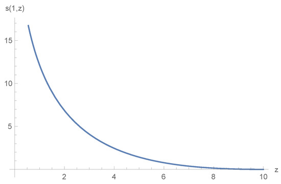
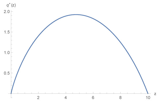
Figure 1 presents the value function of . Apparently, Figure 1 shows that the value function is decreasing and convex on the variable z, which verifies Propositions 1 and 2. Figure 2 shows the optimal policy of the different initial value z at time . As we can see, the reinsurance retention proportion will first increase and then decrease with respect to the wealth. This can explain that when the wealth is close to 0 or close to the target, the insurance company will prefer to transfer all of the risky claims to the reinsurance company and invest money on the risk-less asset.
Figure 1.
The optimal value function s with respect to z at time .
Figure 2.
The optimal reinsurance policy with respect to z at time .
Example 2.
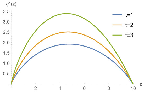
In this example, we use the same parameters as in Example 1, except that we change the time , respectively, and see the effect of the time variable on the optimal policy. Figure 3 shows the optimal reinsurance policy with respect to variable z at different times . As we can see, as time passes, the reinsurance retention proportion increases, which means that the insurance company would like to undertake more risks when the time is close to the deadline.
Figure 3.
The optimal reinsurance policy with respect to z at time .
Example 3.
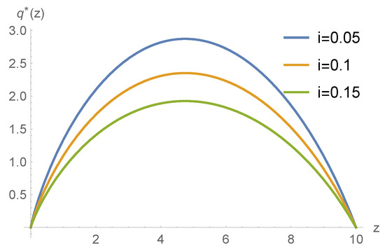
In this example, we use the same parameters as in Example 1, except that we change the interest rate , respectively. Figure 4 shows the effect of different interest rates on the optimal policy. As we can see, as the interest rate increases, the reinsurance retention proportion decreases, which means that the insurance company will prefer to invest more on the risk-less asset when the interest rate increases. This phenomenon is consistent with common sense because when the interest rates rise, investors are more inclined to keep their money in the bank.
Figure 4.
The optimal reinsurance policy with respect to z under different interest rates .
Example 4.
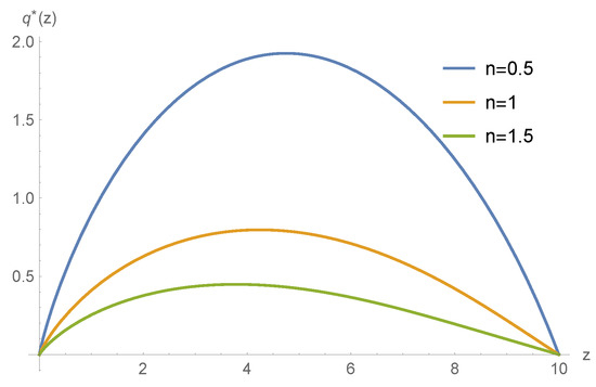
In this example, we use the same parameters as in Example 1 except that we change the diffusion volatility rate . As n increases, the risk of large claims also increases. As shown in Figure 5, as n increases, the reinsurance retention level decreases. In other words, if the claim risk is too high, the insurance company will prefer to transfer risks to the reinsurance company instead of keeping premiums.
Figure 5.
The optimal reinsurance policy with respect to z under different volatility rates .
Example 5.
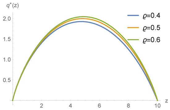
In this example, we still use the same parameters as in Example 1 except the reinsurance safety loading ϱ. Figure 6 shows the optimal reinsurance retention level with different reinsurance safety loadings. The increasing of safety loading means that the reinsurance contract is more expensive. Thus, the optimal choice is to increase the reinsurance retention level so that the insurer can keep more premiums in the insurance company.
Figure 6.
The optimal reinsurance policy with respect to z with different reinsurance safety loading .
Example 6.
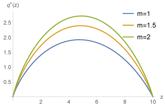
In this example, we still use the same parameters as in Example 1, except we change the expected loss in each unit time , respectively. Figure 7 shows that when m increases, the reinsurance retention level will also increase. This can be explained by the fact that when the parameter m increases, the insurance company obtains more premiums so that the optimal choice for the insurance company is to pull up the insurance retention level.
Figure 7.
The optimal reinsurance policy under different expected losses in unit time .
6. Conclusions
As an application of probability, this paper explores a reinsurance optimization problem that has multiple curved boundaries. To simplify the optimization problem, the technique of changing variables is used. After changing variables, we adopt the dual transformation to solve the new HJB equation. Eventually, an explicit expression of the value function as well as the optimal policy is shown. With some numerical experiments, we list several important influential factors that affect the reinsurance retention level in Table 1. For simplicity, the notation ↑ means “increases” and ↓ means “decreases”. Table 1 shows that the current time, the interest rate, the diffusion volatility rate, the reinsurance safety loading, and the expected loss in unit time will simultaneously affect the optimal reinsurance policy.

Table 1.
Factors that affect reinsurance policy.
Author Contributions
Y.Z. designed the research and wrote the paper. H.H. gave the methodology and the support of funding acquisition. All authors have read and agreed to the published version of the manuscript.
Funding
The work was sponsored by the Natural Science Foundation of Chongqing (cstc2020jcyj-msxmX0762, CSTB2022NSCQ-MSX0290) and the Talent Initial Funding for Scientific Research of Chongqing Three Gorges University (20190020).
Institutional Review Board Statement
Not applicable.
Informed Consent Statement
Not applicable.
Data Availability Statement
The data presented in this study are available upon request from the corresponding author.
Acknowledgments
The authors thank the editor and the referees for their valuable comments and suggestions, which improved greatly the quality of this paper.
Conflicts of Interest
The authors declare no conflict of interest.
References
- Jøjgaard, B.H.; Taksar, M. Controlling risk exposure and dividends payout schemes: Insurance company example. Math. Financ. 1999, 9, 153–182. [Google Scholar] [CrossRef]
- Irgens, C.; Paulsen, J. Optimal control of risk exposure, reinsurance and investments for insurance portfolios. Insur. Math. Econ. 2004, 35, 21–51. [Google Scholar] [CrossRef]
- Hipp, C.; Taksar, M. Optimal non-proportional reinsurance control. Insur. Math. Econ. 2010, 47, 246–254. [Google Scholar] [CrossRef]
- Azcue, P.; Muler, N. Stochastic Optimization in Insurance: A Dynamic Programming Approach; Springer: New York, NY, USA, 2014. [Google Scholar]
- Schmidli, H. Stochastic Control in Insurance; Springer: London, UK, 2008. [Google Scholar]
- Bäuerle, N. Benchmark and mean-variance problems for insurers. Math. Meth. Oper. Res. 2005, 62, 159–165. [Google Scholar] [CrossRef]
- Bielecki, T.R.; Jin, H.; Pliska, S.R.; Zhou, X.Y. Continuous-time mean-variance portfolio selection with bankruptcy prohibition. Math. Financ. 2005, 15, 213–244. [Google Scholar] [CrossRef]
- Bi, J.; Meng, Q.; Zhang, Y. Dynamic mean-variance and optimal reinsurance problems under the no-bankruptcy constraint for an insurer. Ann. Oper. Res. 2014, 212, 43–59. [Google Scholar] [CrossRef]
- Wong, K.C.; Yam, S.C.P.; Zeng, J. Mean-risk portfolio management with bankruptcy prohibition. Insur. Math. Econ. 2019, 85, 153–172. [Google Scholar] [CrossRef]
- Tang, Q. The finite-time ruin probability of the compound Poisson model with constant interest force. J. Appl. Probab. 2005, 42, 608–619. [Google Scholar] [CrossRef]
- Albrecher, H.; Thonhauser, S. Optimal dividend strategies for a risk process under force of interest. Insur. Math. Econ. 2008, 43, 134–149. [Google Scholar] [CrossRef]
- Gao, Q.; Zhuang, J.; Huang, Z. Asymptotics for a delay–claim risk model with diffusion, dependence structures and constant force of interest. J. Comput. Appl. Math. 2019, 353, 219–231. [Google Scholar] [CrossRef]
- Chen, C.; Wang, S. Asymptotic ruin probability for a by–claim risk model with pTQAI claims and constant interest force. Commun. Stat. Theory Methods 2020, 49, 4367–4377. [Google Scholar] [CrossRef]
- Geng, B.; Liu, Z.; Wang, S. On asymptotic finite–time ruin probabilities of a new bidimensional risk model with constant interest force and dependent claims. Stoch. Models 2021, 37, 608–626. [Google Scholar] [CrossRef]
- Liu, X.; Gao, Q. Uniform asymptotics for the compound risk model with dependence structures and constant force of interest. Stochastics 2022, 94, 191–211. [Google Scholar] [CrossRef]
- Liang, X.; Palmowski, Z. A note on optimal expected utility of dividend payments with proportional reinsurance. Scand. Actuar. J. 2018, 4, 275–293. [Google Scholar] [CrossRef]
- Pham, H. Continuous-Time Stochastic Control and Optimization with Financial Applications; Springer: Berlin, Germany, 2009. [Google Scholar]
- Dadashi, H. Optimal investment strategy post retirement without ruin possibility: A numerical algorithm. J. Comput. Appl. Math. 2020, 363, 325–336. [Google Scholar] [CrossRef]
- Di Giacinto, M.; Federico, S.; Gozzi, F.; Vigna, E. Constrained Portfolio Choices in the Decumulation Phase of a Pension Plan. Carlo Alberto Notebooks, No. 155. 2010. Available online: http://ssrn.com/abstract=1600130 (accessed on 21 March 2023).


Disclaimer/Publisher’s Note: The statements, opinions and data contained in all publications are solely those of the individual author(s) and contributor(s) and not of MDPI and/or the editor(s). MDPI and/or the editor(s) disclaim responsibility for any injury to people or property resulting from any ideas, methods, instructions or products referred to in the content. |
© 2023 by the authors. Licensee MDPI, Basel, Switzerland. This article is an open access article distributed under the terms and conditions of the Creative Commons Attribution (CC BY) license (https://creativecommons.org/licenses/by/4.0/).