Article

Spectral Problem of the Hamiltonian in Quantum Mechanics without Reference to a Potential Function

1
Physics Department, King Fahd University of Petroleum & Minerals, Dhahran 31261, Saudi Arabia
2
Saudi Center for Theoretical Physics, Jeddah 21438, Saudi Arabia
*
Author to whom correspondence should be addressed.
Axioms 2023, 12(4), 334; https://doi.org/10.3390/axioms12040334
Submission received: 28 January 2023 / Revised: 17 March 2023 / Accepted: 27 March 2023 / Published: 29 March 2023
(This article belongs to the Special Issue Computation Methods on Quantum Systems)

Abstract

:
Following the celebrated postulates of quantum mechanics, we write the quantum mechanical wavefunction as a convergent series of suitably selected complete square-integrable basis functions in configuration space. The expansion coefficients of the series are energy orthogonal polynomials that contain all spectral information about the system. We exploit the properties of these polynomials to introduce physical systems with rich and highly nontrivial energy spectra. In this approach, no reference is made at all to the usual potential energy function. We consider, in this new approach, a few representative problems at the level of undergraduate students who took at least two courses in quantum mechanics and are familiar with the basics of orthogonal polynomials. Our aim is to expose students to quantum systems with rich energy spectra that goes beyond the very limited textbook examples of systems with very simple energy spectra (e.g., the harmonic oscillator, Coulomb, Morse, Pöschl–Teller, etc.) illustrating the physical significance of these energy polynomials in the description of a quantum system. To assist students, partial solutions are given in an appendix as tables and figures.

1. Introduction

According to the basic postulates of quantum mechanics, a quantum system is fully determined by its space–time wavefunction Ψ ( t , r ) and its Hamiltonian operator H. The wavefunction carries all information needed to calculate the expectation values of operators that represent physical observables. The Hamiltonian, on the other hand, generates the dynamics of the system through the famous Schrödinger equation: i t Ψ = H Ψ [1]. The Hamiltonian operator is the most vital among all observables and its eigenfunction Φ , defined by H Φ = E Φ , has a special place in quantum mechanics. Note that we designated the eigenvalue (measurement of H) as E because the physical unit of H is energy. Combining this eigenvalue equation with the Schrödinger equation gives the corresponding wavefunction for this measurement as Ψ = e i E t / Φ . Therefore, performing all such energy measurements on the system will give its full energy content, called the spectrum { E } . It also gives its total wavefunction as a linear combination (discrete and/or continuous) of all such energy components { e i E t / Φ } 
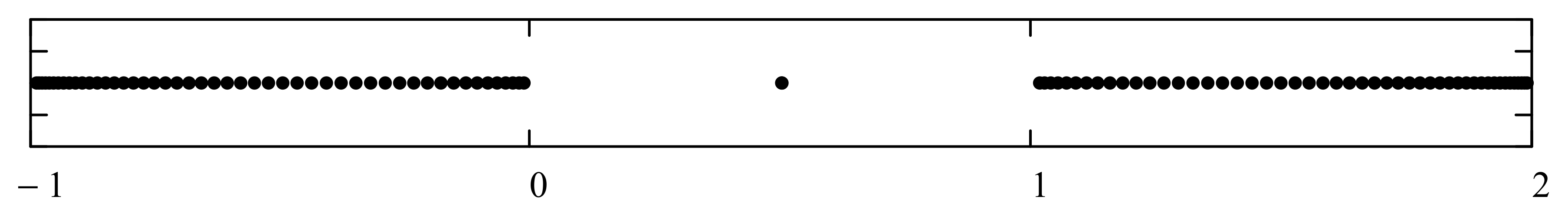
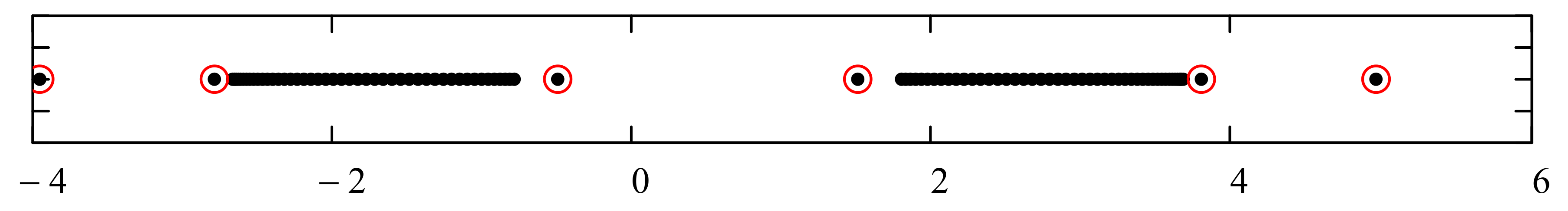
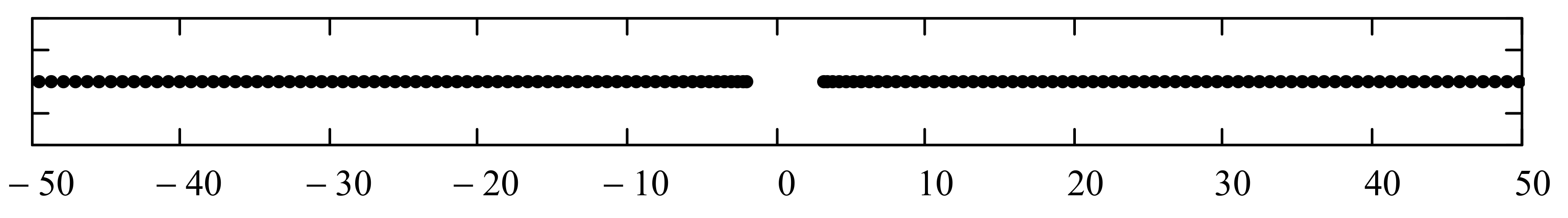
. Due to the extensive physical studies of the energy content of a countless number of quantum mechanical systems and due to parallel extensive mathematical studies of the spectrum of Hermitian operators in Hilbert spaces, people over time have understood very well the nature of the energy spectra. Generally speaking, the energy spectrum of a physical system consists of continuous and discrete parts. The continuous part is usually made up of several disconnected but continuous energy intervals called “energy bands,” which we designate here by the symbol Ω. The discrete part, on the other hand, consists of either a finite or countably infinite set of discrete energy values { E k } . In general, these two sets do not overlap. However, recently the topic of bound states imbedded in the continuum emerged in condensed matter physics [2].
Our starting point in this approach is to represent the total space–time wavefunction Ψ ( t , r ) , which gives full information about the physical system at a given time, by writing its general Fourier expansion over the entire energy spectrum as follows:
Ψ ( t , r ) = Ω e i E t / ψ ( r , E ) d E + k e i E k t / ψ k ( r ) .
Therefore, we assume that the system is fully determined if we can write down its continuous and discrete Fourier components ψ ( r , E ) and ψ k ( r ) . From this point onward, we adopt the atomic units = M = 1 and assume that the quantum mechanical system exists in a one-dimensional configuration space with coordinates x x x + , where x ± are the boundaries of the space.
In the traditional formulation of quantum mechanics, the continuous and discrete parts of the energy spectrum are determined by solving the stationary Schrödinger wave equation. The Hamiltonian operator for a single particle is defined by H = T + V ( x ) = 1 2 d 2 d x 2 + V ( x ) , where V(x) is the potential function that models the system. In this formulation, the Hamiltonian expression is analogous from the Hamiltonian formulation of classical mechanics where the momentum and position are promoted to operators as per first canonical quantization rules. Hence, the concept of a potential energy is deeply rooted in the Hamiltonian formulation of classical mechanics according to which the energy of a particle can always be expressed as the sum of its kinetic energy and potential energy. Since the potential energy of a particle depends on its position, then the potential becomes a function in configuration space and, by construction, it is the only Hamiltonian component that can be related to the classical force concept. For example, the potential function of a massive particle attached to a linear massless spring of constant k is 1 2 k x 2 and the spring force is F = d V d x = k x . The potential function of a particle of mass M moving in the gravitational field of a point mass is M G / r (G being the gravitational constant and r the radial distance to the point mass) and the gravitational force is F = d V ( r ) d r = G M / r 2 , etc. More sophisticated potential functions were also proposed to describe complex systems such as the generalized Morse potential V ( x ) = D ( e 2 μ x 2 α e μ x ) that describes the molecular vibrations of a diatomic molecule with D, α, and μ being physical parameters. This makes it clear that the concept of potential function was carried over from classical to quantum mechanics, through the construction of the system Hamiltonian, despite the fact that none of the postulates of the quantum theory requires it. However, the Aharonov–Bohm (AB) quantum effect defied this general consensus that particle dynamics are solely due to fields at their locations [3]. In particular, the AB effect has shown through a neat double-slit interference experiment that the electromagnetic field can vanish everywhere that the electron moves, but that the electron motion is strongly affected by the electromagnetic interaction. In quantum theory, the AB effect can be explained without the notion of potential function. Thus, one could conclude that the potential function in quantum mechanics might just be a useful auxiliary mathematical tool that can be disposed of after all.
Going back to the main quantum mechanical ingredient, which is the particle wavefunction, we notice that almost all wavefunctions of systems with known exact solutions of the wave equation (e.g., the Coulomb, oscillator, Morse, Pöschl–Teller, etc.) are written in terms of classic hypergeometric orthogonal polynomials in configurations space (such as, Hermite, Laguerre, and Jacobi polynomials). However, an alternative approach to quantum mechanics was recently proposed with the premise that the class of analytically realizable systems is much larger than the exactly solvable class in the conventional potential function formulation [4,5]. This vision proved right and successful as demonstrated in several recent studies [6,7,8,9]. In this alternative approach adopted in the present work, no mention is ever made of a potential function. Consequently, the Hamiltonian operator is not written as the sum H = T + V . Nonetheless, the sacred Fourier expansion in the energy of the wavefunction given in (1) is still maintained. In this approach, the continuous and discrete Fourier energy components are written as the following pointwise convergent series:
ψ ( x , E ) = n = 0 f n ( E ) ϕ n ( x ) ,
ψ k ( x ) = n = 0 g n ( E k ) ϕ n ( x ) ,
where { ϕ n ( x ) } n = 0 is a complete set of square-integrable functions, to be suitably selected shortly, and { f n , g n } 
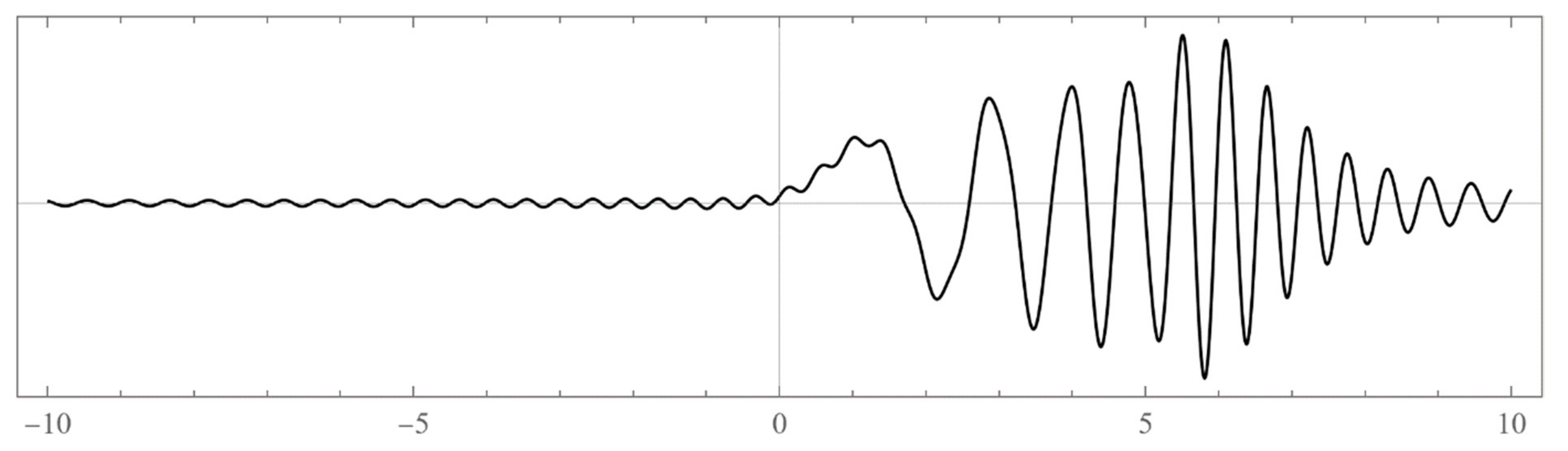
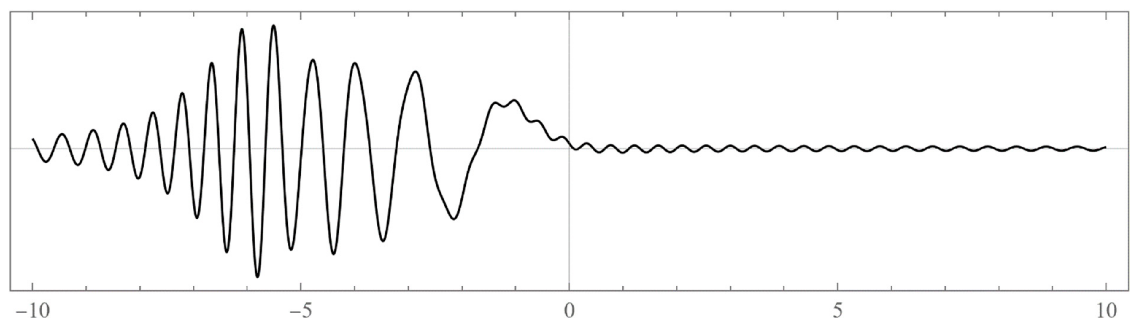
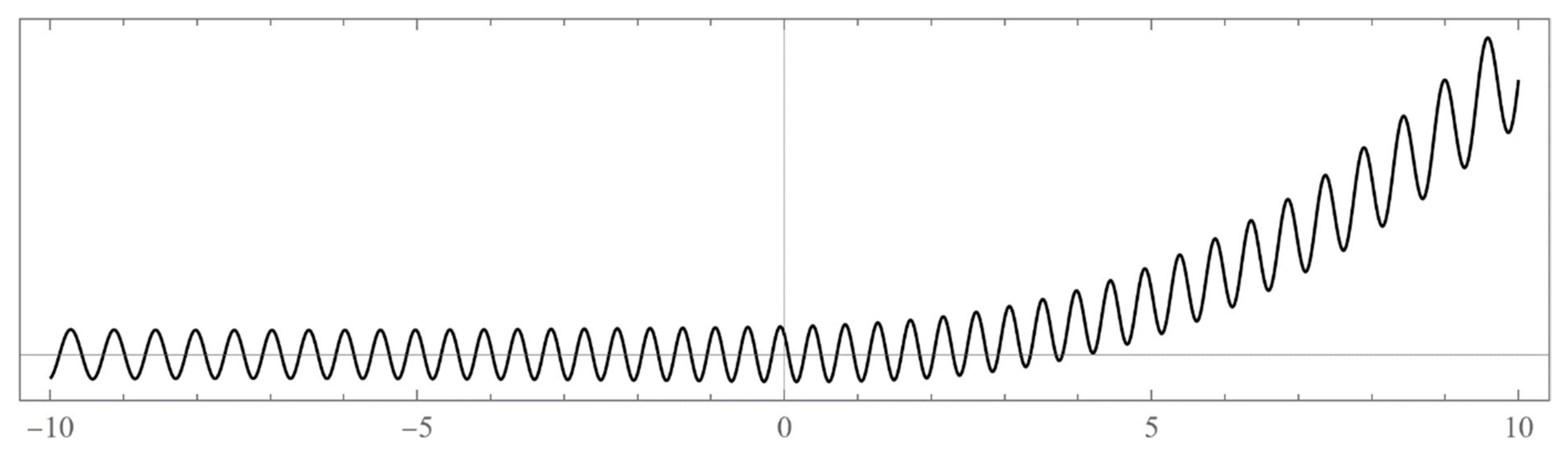
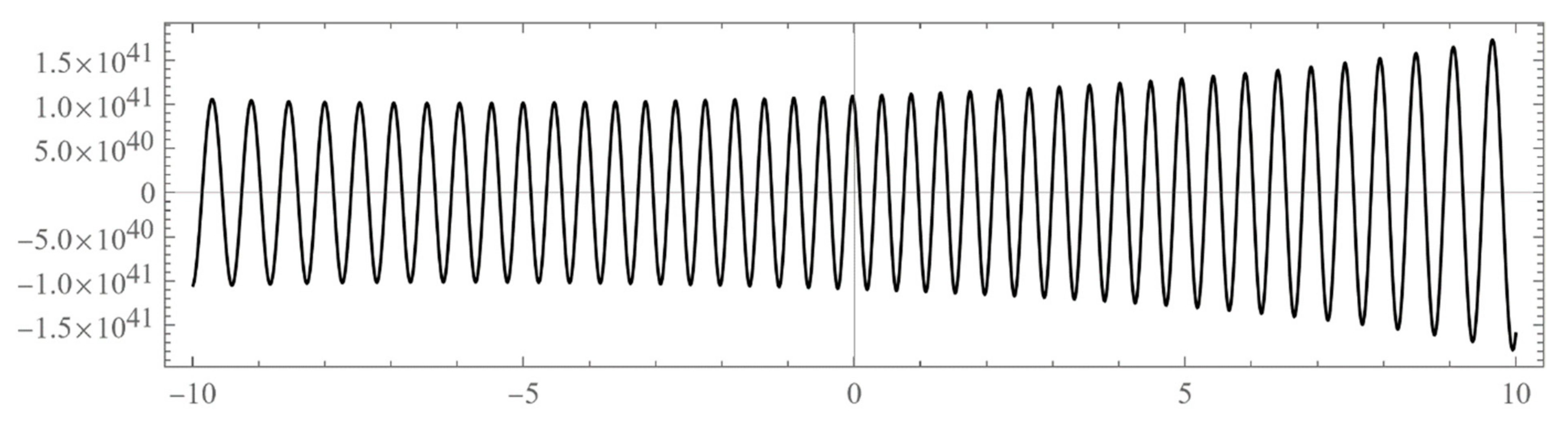
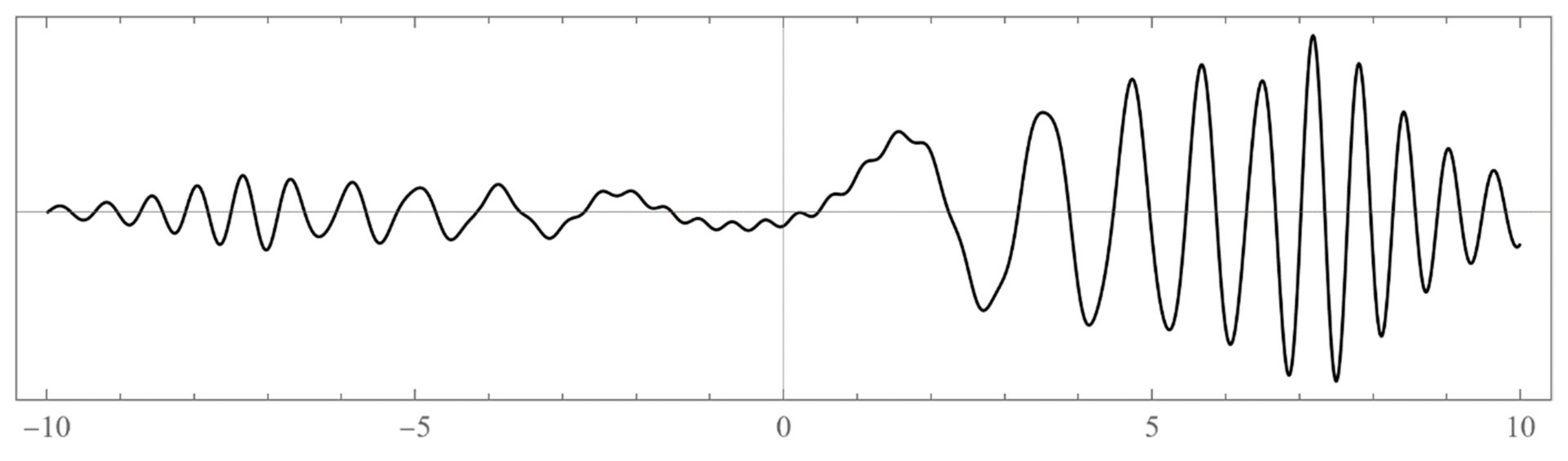
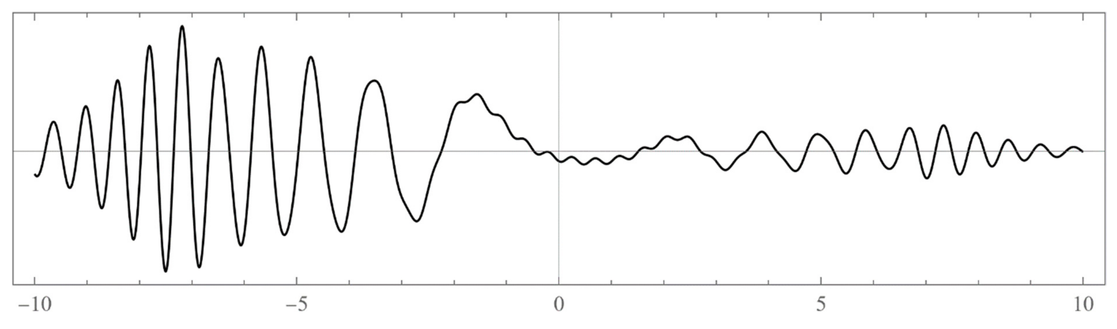
are proper expansion coefficients. The wavefunction (2a) associated with the continuous spectrum is characterized by bounded oscillations that do not vanish all the way to the boundaries of space. However, the wavefunction (2b) associated with bound states is characterized by a finite number of oscillatory-like behavior (with a number of nodes that equals the bound state excitation level 
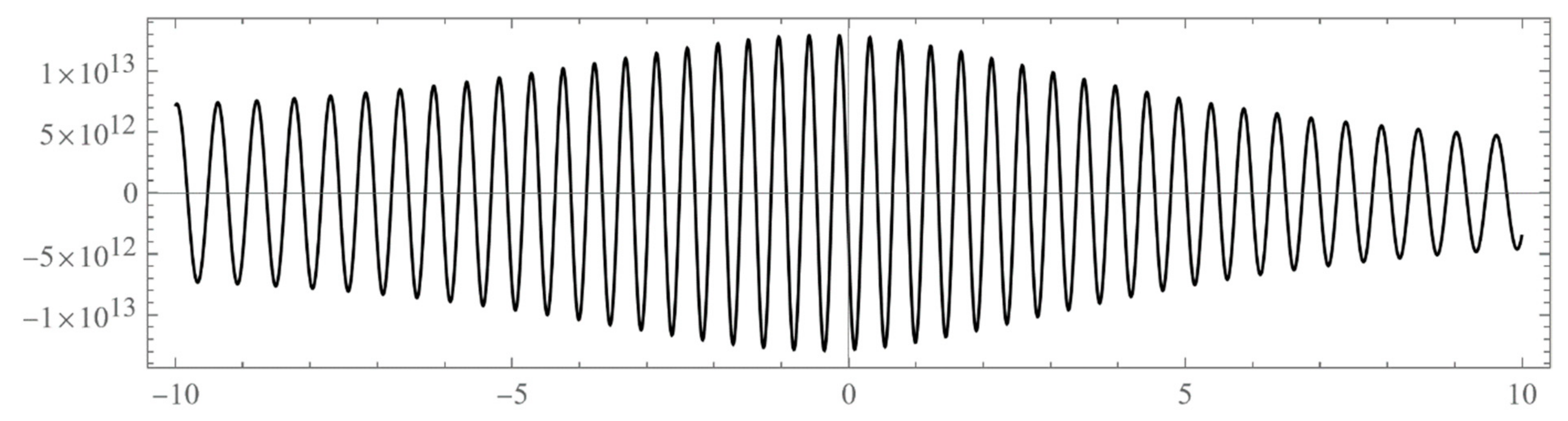
k) that vanishes rapidly at the boundaries. On the other hand, attempting to evaluate the wavefunction at an energy that does not belong to the spectrum will only result in a diverging series. That is, the result is non-stable endless oscillations that grow without bound all over space as the number of terms in the sum increases. Numerically, this is a signature of a nonphysical forbidden value of the selected energy.
We need to stress that in our present approach, we are not trying to reinvent quantum mechanics or propose a new theory. In fact, we are following the celebrated postulates of quantum mechanics exactly. The major novelty in our approach is that we expressed the quantum mechanical wavefunction as a convergent series of a suitably selected complete square integrable basis functions in configuration space that ensure a tridiagonal representation of our Hamiltonian. That is, in our present approach, we impose by construction that the action of the Hamiltonian operator on the basis set will have the following tridiagonal form:
H ϕ n ( x ) = a n ϕ n ( x ) + b n 1 ϕ n 1 ( x ) + b n ϕ n + 1 ( x ) ,
where a n and b n are real constants such that b n 0 for all n. The structure of the off-diagonal elements reflects the Hermitian nature of the Hamiltonian. Therefore, substituting (2a) and (2b) in the Schrödinger wave equation, i t Ψ ( t , x ) = H Ψ ( t , x ) , gives the following algebraic equation for the wavefunction expansion coefficients:
E f n ( E ) = a n f n ( E ) + b n 1 f n 1 ( E ) + b n f n + 1 ( E ) ,
E k g n ( E k ) = a n g n ( E k ) + b n 1 g n 1 ( E k ) + b n g n + 1 ( E k ) .
We should note that so far, the Hamiltonian operator is not assumed to take any specific form such as H = T + V . Note also that the expansion coefficient, a n and b n , are independent of E, as this is obvious from Equation (3); they just represent the matrix elements of H in the basis set { ϕ n ( x ) } n = 0 (if it happens to be an orthonormal set; see Equation (8) below). Generally, the solution of Equation (4a,b) is a polynomial in E, modulo an overall multiplicative arbitrary function of E. Therefore, if we factorize this overall multiplicative function by writing f n ( E ) = f 0 ( E ) P n ( E ) and g n ( E k ) =   g 0 ( E k ) P n ( E k ) , then P n ( E ) will be a polynomial of degree n in E with P 0 ( E ) = 1 . Equations (4a,b) become collectively the following symmetric three-term recursion relation for the energy polynomials { P n ( E ) } n = 0
E P n ( E ) = a n P n ( E ) + b n 1 P n 1 ( E ) + b n P n + 1 ( E ) ,
where E is an element of the total energy spectrum (continuous and discrete). Hence, in this approach, the Schrödinger wave equation in the standard quantum mechanical formulation is replaced by the above three-term recursion relation of the energy orthogonal polynomials.

2. The Energy Polynomials

These polynomials are solutions of the three-term recursion relation (5) for n = 0 , 1 , 2 , with the two initial seed values P 1 ( E ) = 0 and P 0 ( E ) = 1 . The spectral theorem of orthogonal polynomials (also known as the Favard theorem) [10,11] guarantees that with these initial values and the condition b n 0 , they form a complete sequence of orthogonal polynomials satisfying the following general orthogonality relation:
Ω ρ ( E ) P n ( E ) P m ( E ) d E + k ω k P n ( E k ) P m ( E k ) = δ n , m ,
where ρ ( E ) and ω k are the continuous and discrete components of the weight function, respectively (One can write the orthogonality (6) in a compact form as + ξ ( E ) P n ( E ) P m ( E ) d E = δ n , m , where ξ ( E ) = j ρ ( E ) θ ( E , E j ± ) + k ω k δ ( E E k ) and θ ( E , E j ± ) = { 1 , E j E E j + 0 , otherwise   ). One can show that ρ ( E ) = f 0 2 ( E ) and ω k = g 0 2 ( E k ) [4,5,6,7,8,9]. The zeros (roots) of these polynomials play a crucial role in determining some of the most important physical properties of the system, such as the allowed energy bands, density of states, bound state energies, etc. One way to find these zeros is as follows. Construct the following finite n × n tridiagonal symmetric matrix:
R = ( a 0 b 0 b 0 a 1 b 1 b 1 a 2 b 2 × × × × × × b n 3 a n 2 b n 2 b n 2 a n 1 ) .
Then, one can easily show that the zeros of P n ( E ) are the eigenvalues of R. Moreover, due to the special conditions on the recursion coefficients, all these zeros are distinct, in complete agreement with the fact that the 1D Schrödinger equation has no degeneracy. Additionally, the zeros of P n ( E ) interlace within those of P n + 1 ( E ) . Finally, what is left for determining the wavefunction in (1) and (2a,b) is only to know the basis set { ϕ n ( x ) } n = 0 . However, all physical characteristics of the system are contained in the energy polynomials, whereas the basis elements are used only to facilitate realization of the system in configuration space. Moreover, the parameters in the basis elements (if any) are either derived from the physical parameters in the energy polynomials or they are non-physical and could be used to improve computations. Thus, in this approach to quantum mechanics, a physical model is defined not by any potential function but by giving the pair { P n ( E ) , ϕ n ( x ) } . Moreover, one may specify the set { a n , b n } n = 0 as alternative to { P n ( E ) } n = 0 . Note, that if we adopt the potential picture and write H = T + V , then for a given set { a n , b n } n = 0 , the solution of Equation (3) for proper boundary conditions will determine the basis set { ϕ n ( x ) } n = 0 . However, in this alternative approach to quantum mechanics, Equation (3) which is equivalent to the recursion relation (5), is considered as an algebraic definition of the Hamiltonian in place of H = T + V . In fact, if the basis set is orthonormal (i.e., ϕ n | ϕ m = δ n , m ), then Equation (3) gives the following matrix representation of the Hamiltonian:
H n , m = ϕ n | H | ϕ m = a n δ n , m + b n 1 δ n , m + 1 + b n δ n , m 1 .
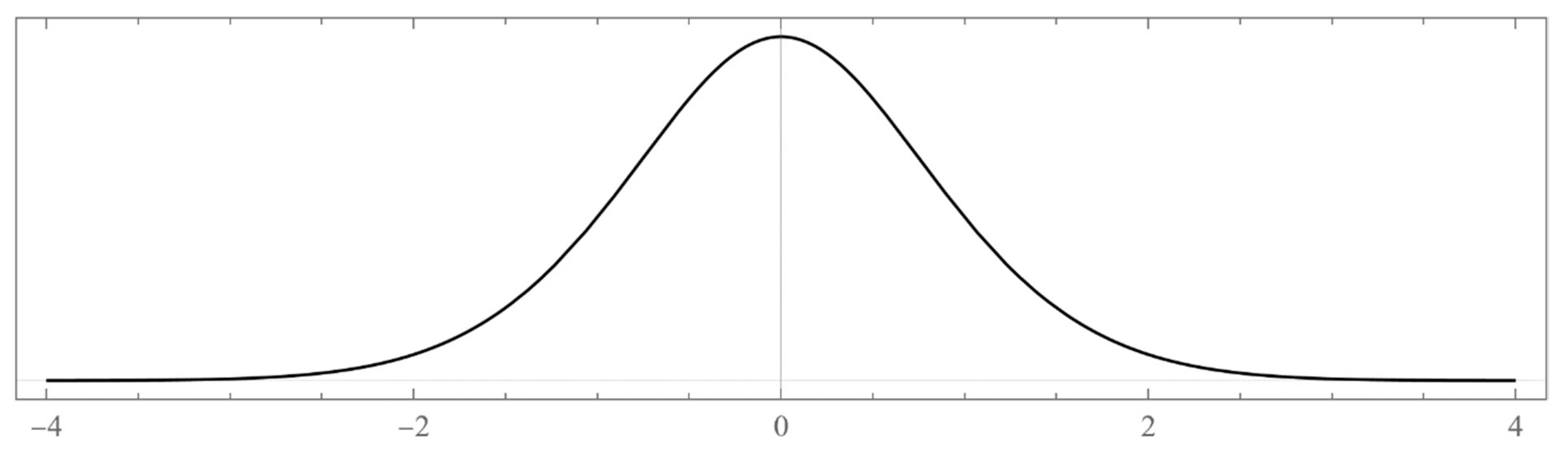
That is, the tridiagonal symmetric matrix (7) is a finite n × n submatrix representation of H. In the absence of any explicit constraint on the basis functions { ϕ n ( x ) } n = 0 (aside from square-integrability and completeness), we write them in a general form as ϕ n ( x ) = W ( y ) Q n ( y ) , where y = y ( x ) is a coordinate transformation, Q n ( y ) is a classic polynomial of degree n in y, and W ( y ) is a positive weight function designed to satisfy W ( y ± ) = 0 , where y ± = y ( x ± ) . Usually, y ( x ) takes us from the physical configuration space to the desirable finite or semi-infinite domains compatible with those of the polynomials Q n ( y ) .
In Section 3 and Section 4, we propose several problems within this approach to quantum mechanics. These are aimed at undergraduate students who took at least two courses of quantum mechanics and are familiar with the basics of orthogonal polynomials. To avoid any remarkable prerequisites in advanced quantum mechanics and/or mathematical analysis, the problems were designed with emphasis on the numerical aspect rather than the analytical aspect of the solution. For example, we provide an equivalent description of the orthogonal energy polynomials by giving their three-term recursion relation vis-à-vis the recursion coefficients { a n , b n } . Consequently, we just stress the importance of the structure of the recursion coefficients { a n , b n } in the three-term recursion relation (5). That is, we define the orthogonal energy polynomials through their recursion relation and initial values rather than through their analytic properties (e.g., weight function, generating function, Rodrigues formula, etc.). By doing so, we avoid mentioning the explicit form of these energy polynomials and their associated analytical properties which go beyond undergraduate level. Therefore, we use the three-term recursion relation and its coefficients as a defining tool for the associated energy polynomials. In particular, we want the students to become familiar with the key role played by the recursion coefficients { a n , b n } and how their asymptotic behavior affects the corresponding energy spectrum. Not only that, but the same coefficients are sufficient in determining important physical properties such as the density of states, a property that describes how closely packed energy levels are in a given system, which plays a pivotal role in computing transport properties of physical systems [12].
In the illustrative examples considered in this work, the configuration space is either the whole real line (Section 3) or only the non-negative part of the real line (Section 4) where we give a suitable square integrable basis set for each situation. Partial solutions for these examples are given in Appendix A in the form of figures and tables. Since the proposed problems are aimed at undergraduate students, we assume general rather than specialized knowledge of orthogonal polynomials.
Before we embark on computations related to specific problems, it is instructive at this point to digress on the numerical computations of the bound state energies. These are located outside the continuous energy bands and can be defined using any one of the following prescriptions:
i.
The set of energies { E k } that satisfy: lim n P n ( E k ) = 0 . That is, E k is an asymptotic zero for all energy polynomials in the limit of infinite (large enough) degrees (If for a particular value of the energy, P n ( E ^ ) = 0 for all n (not only asymptotically) then E ^ is not the energy of a bound state. In fact, this property makes the energy polynomials non-orthogonal. If we remove this zero by defining P n ( E ) = ( E E ^ ) Q n 1 ( E ) then the polynomials { Q n ( E ) } will form a true orthogonal sequence of energy polynomials).
ii.
The set of eigenvalues of the tridiagonal matrix (7) that lie outside the energy bands and do not change significantly (within the desired accuracy) if we vary the size of the matrix around a large enough size N × N . (It may happen that an eigenvalue E ^ of the matrix (7), which lies isolated outside the energy bands or in an energy gap, does not correspond to a bound state. It is advisable that one evaluates the polynomial at all such eigenvalues and performs the test lim n P n ( E ^ ) = 0 ).
iii.
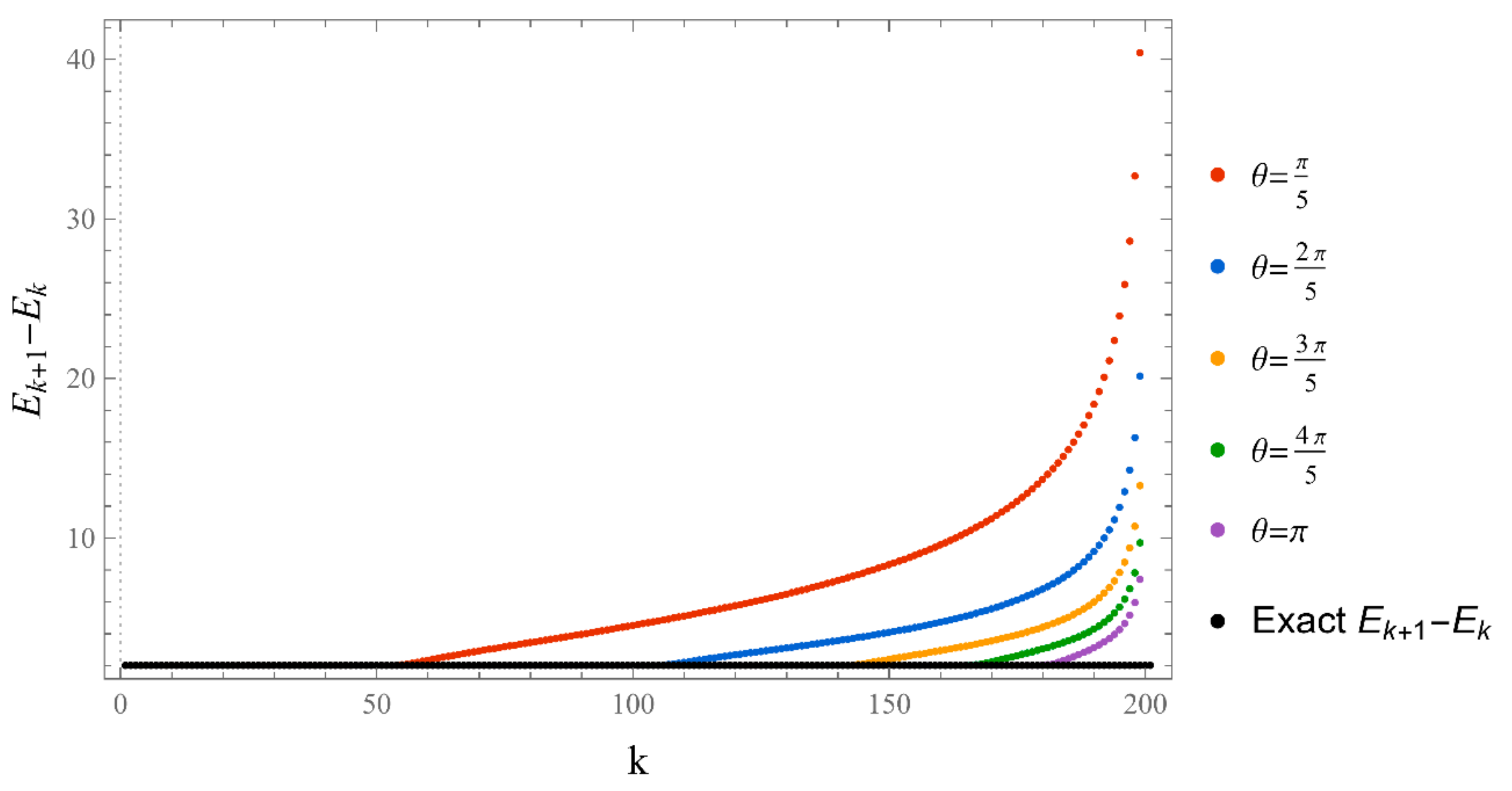
The set of energies that make the asymptotic limit ( n ) of the polynomial P n ( E ) vanish (Typically, these asymptotics take the form P n ( E ) 1 n α ρ ( E ) cos [ n β φ ( E ) + δ ( E ) ] , where α and β are positive real parameters, ρ ( E ) is the weight function, φ ( E ) is an entire function, and δ ( E ) is the scattering phase shift. If β 0 then n β ln ( n ) . As an illustration, we plot P n ( E ) as a function of n for a fixed E from within the bands in Problem II and verify the oscillatory behavior of the asymptotics (we take, for example, E =   λ 2 { 1.9 , 0.5 } ). We also show that the asymptotics in fact vanishes at the energy = λ 2 / 2 ).
However, since this manuscript is mainly addressed to undergraduate students, we have opted to use mainly the simple computational scheme (ii) based on matrix eigenvalues, which is a very much familiar problem to undergraduate students. Nevertheless, sometimes scheme (ii) produces erroneous results. Thus, if in doubt, one needs to double-check and independently verify the viability of the bound states using the asymptotic schemes (i) or (iii) (see, for example, problem III and Figure A12).
As it is now evident from the discussion above, the energy polynomials are totally determined if the recursion coefficients { a n , b n } and the two initial values { P 1 ( E ) , P 0 ( E ) } are given because then a unique polynomial solution of the three-term recursion relation (5) is obtained. The large n asymptotic values of { a n , b n } play an important role in determining the allowed energy intervals that the system can occupy (called “energy bands”). Moreover, these asymptotic values uniquely determine the boundaries of these energy bands. In fact, if this asymptotic limit is multivalued, that is lim n { a n , b n } = { A j , B j } j = 1 J with J being a positive integer number, then the continuous energy spectrum consists of J disconnected but continuous energy bands with J 1 gaps in between. Under these conditions, the infinite version of the matrix (7), which represents the Hamiltonian matrix, will have a tail consisting of identical J × J tridiagonal block matrices (with As on the diagonal and Bs on the off-diagonal) that repeats forever. If one or more of the asymptotic values { A j , B j } is/are infinite, then the size of some or all of the bands is also infinite. All points within the bands correspond to energies within the continuous scattering energy states. Bound states (if they exist) have energies that correspond to discrete points located outside the energy bands (inside the gaps or beyond the bands). We refer advanced readers to reference [13] for all necessary mathematical details related to the computations of the asymptotic limits lim n { a n , b n } = { A j , B j } j = 1 J and how they are used to define the boundaries of the energy bands.

3. Problems in the Infinite Domain

For the first set of problems, the configuration space is considered to be the whole real line where x ± = ± . Under such circumstances, we select the following suitable basis elements:
ϕ n ( x ) = λ / π 2 n n ! e λ 2 x 2 / 2 H n ( λ x ) ; x ] , + [ ,
where H n ( λ x ) is the Hermite polynomial of degree n and λ is a real positive parameter of inverse length dimension which represents an extra free parameter that helps in improving the convergence of the numerical computations once judiciously chosen. These basis elements are orthonormal since ϕ n | ϕ m = + ϕ n ( x ) ϕ m ( x ) d x = δ n , m . In the traditional potential formulation of quantum mechanics, the functions (9) are typically associated with the eigenfunctions of the one-dimensional harmonic oscillator whose energy spectrum is discrete, infinite, and bounded from below. However, in our present context, they are considered as elements of a complete basis set suitable for a wider range of analytical problems that may have discrete as well as continuous energy spectra.

3.1. Problem I

As stated above, if the coefficient of the recursion relation (5) has a single finite asymptotic limit, lim n a n = A and lim n b n = B , then it can be shown that the continuous energy spectrum of the corresponding Hamiltonian will consist of a single energy band with Ω [ A 2 B , A + 2 B ] . Take, for instance, a n = 0 and b n = λ 2 / 2 , which gives Ω [ λ 2 , + λ 2 ] . Calculate the zeros of P N ( E ) for large-enough N which are just the eigenvalues of the tridiagonal matrix (7) and show that the zeros do, in fact, lie within this energy band (shown in Table A1). The un-normalized wavefunction at an energy E is
ψ ˜ ( x , E ) : = n = 0 N P n ( E ) ϕ n ( x ) .
Plots of this function at the energies E = 0 , E = ± λ 2 / 2 and E = ± λ 2 are shown in Figure A2, Figure A3, Figure A4 and Figure A5. Figure A1 shows the zeros of the energy polynomial P N ( E ) in units of λ 2 for N = 100 and Table A1 shows the edges of the allowed energy band as we increase the degree of the polynomial N. If one tries to plot the wave function at | E | > λ 2 , that is outside the energy band, then the wavefunction will blow up—an indication that it is a forbidden energy state of the system as shown in Figure A6 for E = 3 λ 2 / 2 . For completeness, we would like to mention that the orthogonal energy polynomial associated with these recursion coefficients is the normalized version of the Chebyshev polynomial. Moreover, the initial values P 1 ( E ) = 0 and P 0 ( E ) = 1 make it the Chebyshev polynomial of the second kind U n ( E ) [14].

3.2. Problem II

We consider the orthogonal polynomial defined by the following recursion coefficients: a n = λ 2 / 2 , b 2 n = λ 2 2 ( n + 1 2 ) / ( n + 2 ) and b 2 n + 1 = λ 2 . In this case, the continuous energy spectrum will consist of two energy bands since lim n b n = λ 2 { 1 2 , 1 } , where the limits in the parentheses are for even and odd n, respectively. The zeros of P N ( E ) for large-enough N and the associated four boundaries of these two bands are shown explicitly in Figure A7 for N = 100 while the edges of the allowed energy bands are computed in Table A2 for different values of the degree of the polynomial. You will notice, however, that one of the zeros is isolated inside the energy gap between the two bands (in fact, it is located at the middle of the energy gap). This energy is associated with a bound state; let us call this energy and plot ψ ˜ ( x , ) , as shown in Figure A8. This should be a remarkable observation by the students: the basis (9), which is normally associated with the harmonic oscillator whose energy spectrum consists of an infinite number of discrete bound states, is now associated with this system that has only one bound state and two continuous energy bands.
We plot ψ ˜ ( x , E ) for an energy from within the left band and another from the right band as shown in Figure A9 and Figure A10, respectively. We also evaluate the wavefunction ψ ˜ ( x , E ) at an energy from within the forbidden gap but not equal to the bound state energy as shown in Figure A11, which shows extremely large unbounded oscillation all over the space due to the forbidden nature of the selected energy, E = λ 2 / 4 , within the energy gap region.

3.3. Problem III

In this problem, we generalize Problem II by parametrizing the recursion coefficients { a n , b n } as follows:
a 2 n = α λ 2 ,                   a 2 n + 1 = ( 1 α ) λ 2 ,
b 2 n = λ 2 2 β ( n + γ 1 ) / ( n + γ ) ,                     b 2 n + 1 = λ 2 2 γ ( n + β ) / ( n + β 1 ) .
Problem II corresponds to α = 1 2 , β = 1 and γ = 2 . Note that the asymptotic limits of a n and b n are multi-valued. In fact, lim n a n = λ 2 { α , 1 α } and lim n b n = 1 2 λ 2 { β , γ } . Therefore, as stated at the end of Section 2 above, we expect the continuous energy spectrum to consist of two energy bands of finite size. In fact, one can show that the four boundaries of the two energy bands are as follows:
λ 2 2 [ 1 ± ( 2 α 1 ) 2 + ( β + γ ) 2 ] ,         λ 2 2 [ 1 ± ( 2 α 1 ) 2 + ( β γ ) 2 ] .
This result is verified numerically in Table A3 by taking large-enough N. The zeros of this polynomial are shown in Figure A12 for N = 100 and the wavefunction ψ ˜ ( x , E ) is shown in Figure A13 for the bound state at E = 3 λ 2 / 2 and for N = 100 . The corresponding quantum mechanical system is parameterized by the four physical parameters { λ , α , β , γ } . These parameters could be adjusted to fit experimental measurements of the desired system that can be modeled by these energy polynomials.

3.4. Problem IV

Let us construct another two-energy-band system as follows:
a 2 n = α λ 2 ,         a 2 n + 1 = ( 1 α ) λ 2 ,         b 2 n = α λ 2 2 n + β ,         b 2 n + 1 = α λ 2 2 n + γ .
Note that the large degree asymptotic ( n ) limit of b n goes to infinity as n . Consequently, the two energy bands will have infinite sizes whereas the two boundaries of the energy gap are set at λ 2 2 ( 1 ± | 2 α 1 | ) ; this is verified numerically in Table A4. The zeros of P N ( E ) in units of λ 2 are shown in Figure A14 for α = 3 and N = 200 , which shows that the energy bands extend to infinity and the gap is located in the interval 2 λ 2 < E < + 3 λ 2 with no bound states.

4. Problems in the Semi-Infinite Domain

For the second set of problems, the configuration space is considered to be the non-negative part of the real line, x = 0 and x + . This situation will, in particular, be suitable for the radial part of the Schrödinger equation in three dimensions with spherical symmetry. Under such circumstances, we select the following orthonormal basis elements:
ϕ n ( r ) = 2 λ Γ ( n + 1 ) Γ ( n + ν + 1 ) ( λ r ) ν + 1 2 e λ 2 r 2 / 2 L n ν ( λ 2 r 2 ) ,
where L n ν ( z ) is the Laguerre polynomial and the parameters { ν , λ } are to be chosen such that ν > 1 . This basis forms an orthonormal set since 0 ϕ n ( r ) ϕ m ( r ) d r = δ n , m . Again, we note that in the traditional formulation of quantum mechanics and with ν = + 1 2 , the functions (14) are typically associated with the eigenfunctions of the radial Schrödinger equation of a spherically symmetric harmonic oscillator (isotropic oscillator) whose energy spectrum is discrete, infinite, and bounded from below. If ν = 2 + 1 and λ 2 r 2 λ r , then the basis (14) becomes associated with the Coulomb potential for the hydrogen atom whose energy spectrum consists of a combination of a single infinite continuous band with E 0 and an infinite set of discrete energies bounded from below at E = | E 0 | and from above at E = 0 . However, in our present context, these eigenfunctions are taken as the basis set for a wider range of analytical problems that may have discrete as well as continuous energy spectra and may be bounded or unbounded.

4.1. Problem V

We start by reproducing the results associated with the isotropic oscillator problem in this alternative approach to quantum mechanics. For that, the recursion coefficients of the associated orthogonal energy polynomial are chosen as follows:
a n = 2 ω tanh θ ( n + μ ) ,         b n = ω sinh θ ( n + 1 ) ( n + 2 μ ) ,
where ω is the oscillator frequency and 2 μ = + 3 2 . The angular parameter θ , being real and positive, is arbitrary but chosen to improve conversion of the calculation. We verify that the zeros are, in fact, discrete (see, Figure A15) and for large-enough N they converge to the isotropic oscillator energy spectrum:
E k = ω ( 2 k + + 3 2 ) .
Figure A16 shows that the difference between two consecutive states is constant and equal to 2 ω . However, it diverges quickly due to numerical errors, but it becomes more accurate as the value of θ increases. Moreover, the linear dependence of E k on k is shown in Figure A17, and it exhibits the same divergence behavior. Theoretically, the proper choice for this parameter is given by cosh θ = ω 2 + ( λ / 2 ) 4 ω 2 ( λ / 2 ) 4 with λ < 2 ω . By the way, the orthogonal energy polynomial whose recursion coefficients are given by (15) for this problem with discrete spectrum is the Meixner polynomial M n μ ( z k ; θ ) , with z k = E k / 2 ω [14].

4.2. Problem VI

For this problem, we would like to construct an energy spectrum that consists of a semi-infinite continuous band ( E 0 ) and a finite set of discrete negative energies { E k } . To that end, we take the recursion coefficients as follows:
a n = λ 2 [ ( n + μ + γ ) 2 + n ( n + 2 γ 1 ) μ 2 ] ,
b n = λ 2 ( n + μ + γ ) ( n + 1 ) ( n + 2 γ ) ,
where μ < 0 and γ > μ . We verify for γ = 10 , μ = 9.5 that, indeed, the energy spectrum consists of an infinite continuous positive energy band with E 0 (as shown in Figure A18) and a finite number of negative discrete energies (as shown in Figure A19). In addition, the number of the discrete bound state energies is μ , where x stands for the largest integer less than or equal to x. In the large degree N limit, we verify in Figure A20 that for E < 0 , these discrete energies approach the following values:
E k = λ 2 ( k + μ ) 2 ,
where k = 0 , 1 , , μ . Some un-normalized wavefunction ψ ˜ ( r , E k ) are shown in Figure A21 for different k values. These wavefunctions are physically acceptable; that is, they have k nodes and vanish rapidly at the boundaries ( r = 0 and r ). The un-normalized wavefunction ψ ˜ ( r , E ) for E > 0 is shown in Figure A22 and verified to represents a continuous scattering state; that is, bounded oscillations that extends to infinity. By the way, the orthogonal energy polynomial whose recursion coefficients are given by (17a,b) is a special case of the continuous dual Hahn polynomial S n μ ( E ; γ , γ ) [14].

5. Conclusions

From the outset, we like to reiterate and ascertain that we are not reinventing quantum mechanics or proposing a new theory. We are, in fact, following exactly the celebrated postulates of quantum mechanics with the objective of exposing the undergraduate student of quantum mechanics to a larger class of problems with rich energy spectra that goes beyond the simple textbook examples. The major novelty in our approach is that we expressed the quantum mechanical wavefunction as a convergent series of a suitably selected complete square integrable basis functions in configuration space. The expansion coefficients of the series were designed to be orthogonal polynomials in the energy domain and were found to contain all spectral information about the system. For the implementation of our approach, we suitably selected two basis sets that are appropriate for infinite and semi-infinite domains along with a variety of recursion coefficients and showed how the asymptotic behavior of these coefficients play a crucial role in determining the nature of the system energy spectrum. We stressed throughout the manuscript the fact that in the present approach, no reference is made at all to the usual potential energy function. We have demonstrated the validity of this quantum mechanical approach and its power to generate a wide span of rich energy spectra illustrating the physical significance of these energy polynomials in the description of quantum systems. For clarity, we have investigated few representative models that gave rise to a variety of discrete and continuous energy spectra. However, to keep the manuscript at the undergraduate level, all along our manuscript we have avoided talking about the analytical properties of the associated orthogonal polynomials but rather considered their equivalent representation in terms of recursion coefficients { a n , b n } and initial values. We also alluded to the fact that the computation of the system density of states is very easy to handle in the new approach since any three-term recursion relation can be easily written in term of continued fractions, which can be directly related to the DOS.

Author Contributions

Conceptualization, I.F.A.-Y., M.E., H.B. and A.D.A.; Formal analysis, H.B. and A.D.A.; Methodology, H.B. and A.D.A.; Project administration, H.B.; Supervision, H.B. and A.D.A.; Validation, I.F.A.-Y., M.E. and A.D.A.; Visualization, I.F.A.-Y., M.E. and A.D.A.; Writing—original draft, H.B. and A.D.A.; Writing—review & editing, I.F.A.-Y., M.E., H.B. and A.D.A. All authors have read and agreed to the published version of the manuscript.

Funding

This research received no external funding.

Data Availability Statement

Not applicable.

Acknowledgments

We acknowledge the support of King Fahd University of Petroleum and Minerals (KFUPM) during the progress of this research. Alhaidari acknowledges the additional support of the Saudi Center for Theoretical Physics.

Conflicts of Interest

The authors declare no conflict of interest.

Appendix A. Partial Solutions

Appendix A.1. Problem I

Figure A1. The zeros of P N ( E ) in units of λ 2 for N = 100 .
Axioms 12 00334 g0a1
Table A1. The left and right boundaries of the energy band in units of λ 2 for different values of N. The exact values are ± λ 2 .
NLeft BoundaryRight Boundary
10−0.9594930.959493
20−0.9888310.988831
50−0.9981030.998103
100−0.9995160.999516
200−0.9998780.999878
Figure A2. The un-normalized wavefunction ψ ˜ ( x , E ) for E = 0 at the middle of the band. The horizontal x-axis is in units of λ 1 . We took N = 100 .
Axioms 12 00334 g0a2
Figure A3. The un-normalized wavefunction ψ ˜ ( x , E ) for E = + λ 2 / 2 . We took N = 100 .
Axioms 12 00334 g0a3
Figure A4. The un-normalized wavefunction ψ ˜ ( x , E ) for E = λ 2 / 2 . We took N = 100 .
Axioms 12 00334 g0a4
Figure A5. The un-normalized wavefunction ψ ˜ ( x , E ) for E = λ 2 , which is at the right edge of the energy band. We took N = 100 .
Axioms 12 00334 g0a5
Figure A6. The un-normalized wavefunction ψ ˜ ( x , E ) for E = 3 λ 2 / 2 , which is a forbidden energy outside the band. We took N = 100 . Note the unbounded oscillations everywhere.
Axioms 12 00334 g0a6

Appendix A.2. Problem II

Figure A7. The zeros of P N ( E ) in units of λ 2 for N = 100 .
Axioms 12 00334 g0a7
Table A2. The boundaries of the left and right energy bands in units of λ 2 for different values of N. The exact values are λ 2 , 0, λ 2 , and 2 λ 2 .
NLeft BoundariesRight Boundaries
20−0.926138−0.1057991.1057991.926138
50−0.973840−0.0347241.0347241.97384
100−0.988118−0.0149081.0149081.988118
200−0.994550−0.0065171.0065171.99455
400−0.997467−0.0029151.0029151.997467
Figure A8. The un-normalized wavefunction ψ ˜ ( x , ) for the bound state in the middle of the energy gap with = 1 2 λ 2 . The horizontal x-axis is in units of λ 1 . We took N = 100 .
Axioms 12 00334 g0a8
Figure A9. The un-normalized wavefunction ψ ˜ ( x , E ) for E = 3 λ 2 / 2 in the right energy band. We took N = 100 .
Axioms 12 00334 g0a9
Figure A10. The un-normalized wavefunction ψ ˜ ( x , E ) for E = λ 2 / 2 in the left energy band. We took N = 100 .
Axioms 12 00334 g0a10
Figure A11. The un-normalized wavefunction ψ ˜ ( x , E ) for E = λ 2 / 4 , which is a forbidden energy in the gap. We took N = 100 . Note the unbounded oscillations everywhere.
Axioms 12 00334 g0a11

Appendix A.3. Problem III

Figure A12. The zeros of P N ( E ) in units of λ 2 for N = 100 . We took α = 1.5 , β = 2.3 and γ = 3.7 . Out of the six isolated eigenvalues (shown with red circles) only E = 3 λ 2 / 2 pass the asymptotic test (2.iii) and corresponds to a bound state.
Axioms 12 00334 g0a12
Table A3. The left and right boundaries of the left and right energy bands in units of λ 2 for different values of N. The exact values are in (12).
NLeft BoundariesRight Boundaries
20−2.61667−1.024332.024333.61667
50−2.65286−0.814451.814453.65286
100−2.65775−0.7602551.760263.65775
200−2.6601−0.7379581.737963.6601
300−2.6609−0.7314691.731473.6609
Exact−2.66228−0.7206561.720663.66228
Figure A13. The un-normalized wavefunction ψ ˜ ( x , E ) for the bound state inside the energy gap with E = 3 λ 2 / 2 . The horizontal x-axis is in units of λ 1 . We took N = 100 .
Axioms 12 00334 g0a13

Appendix A.4. Problem IV

Figure A14. The zeros of P N ( E ) in units of λ 2 for N = 200 . We took α = 3 , β = 2 and γ = 1 . The energy bands extend to infinity and the gap is located in the interval 2 λ 2 < E < + 3 λ 2 . The system has no bound states.
Axioms 12 00334 g0a14
Table A4. The left and right boundaries energy gap in units of λ 2 for different values of N. We took α = 3 , β = 2 and γ = 1 . The exact values are λ 2 2 ( 1 ± | 2 α 1 | ) .
NGap Boundaries
20−2.545923.54592
50−2.251553.25155
100−2.133573.13357
200−2.069173.06917
300−2.046723.04672
Exact−2.000003.00000

Appendix A.5. Problem V

Figure A15. The zeros of P N ( E ) in units of λ 2 for different values of N. We took ω = 3 / 2 , μ = 5 / 4 , and θ = π . The energies are found to converge to a discrete equally spaced spectrum.
Axioms 12 00334 g0a15
Figure A16. The difference between consecutive zeros of P N ( E ) for N = 200 . We took ω = 1 , μ = 5 , for different values of θ. The difference is constant, which matches the theoretical value of 2 ω . However, we get better convergence as θ increases.
Axioms 12 00334 g0a16
Figure A17. The kth zero of P N ( E ) vs k for N = 200 . We took ω = 1 , μ = 5 , for different values of θ. This shows how the plot have better convergence as θ increases.
Axioms 12 00334 g0a17

Appendix A.6. Problem VI

Figure A18. The zeros of P N ( E ) in units of λ 2 for N = 200 . We took γ = 10 and μ = 9.5 . The energy bands for E 0 extend to infinity.
Axioms 12 00334 g0a18
Figure A19. The zeros of P N ( E ) in units of λ 2 for different values of N. The energy bands for E < 0 are found to converge to a discrete linearly spaced spectrum.
Axioms 12 00334 g0a19
Figure A20. The kth zero of P N ( E ) vs k for N = 500 . We took γ = 10 and μ = 9.5 . When E < 0 , the zeros of P N ( E ) agrees with Equation (18) up to k = μ .
Axioms 12 00334 g0a20
Figure A21. The un-normalized wavefunction ψ ˜ ( r , E k ) for different values of k . The horizontal r-axis is in units of λ 1 . We took μ = 15 ,   γ = 16 , and ν = 1 . We can observe each wavefunction having k nodes, and vanishes at the boundaries.
Axioms 12 00334 g0a21
Figure A22. The un-normalized wavefunction ψ ˜ ( r , E ) for N = 100 . We took E = 150 λ 2 , for μ = 15 ,   γ = 16 , and ν = 2 . We can see the bounded oscillations that extends to infinity.
Axioms 12 00334 g0a22

References

  1. Galindo, A.; Pascual, P.; Garcia, J.D.; Alvarez-Gaume, L. Quantum Mechanics I; Springer: Berlin/Heidelberg, Germany, 1990. [Google Scholar]
  2. Sadreev, A.F. Interference traps waves in an open system: Bound states in the continuum. Rep. Prog. Phys. 2021, 84, 055901. [Google Scholar] [CrossRef] [PubMed]
  3. Vaidman, L. Role of potentials in the Aharonov-Bohm effect. Phys. Rev. A 2012, 86, 040101(R). [Google Scholar] [CrossRef] [Green Version]
  4. Alhaidari, A.D.; Ismail, M.E.H. Formulation of quantum mechanics without potential function. Quantum Phys. Lett. 2015, 4, 51. [Google Scholar]
  5. Alhaidari, A.D.; Ismail, M.E.H. Quantum mechanics without potential function. J. Math. Phys. 2015, 56, 072107. [Google Scholar] [CrossRef] [Green Version]
  6. Alhaidari, A.D.; Taiwo, T.J. Wilson-Racah Quantum System. J. Math. Phys. 2017, 58, 022101. [Google Scholar] [CrossRef] [Green Version]
  7. Alhaidari, A.D. Reconstructing the potential function in a formulation of quantum mechanics based on orthogonal polynomials. Commun. Theor. Phys. 2017, 68, 711. [Google Scholar] [CrossRef]
  8. Alhaidari, A.D.; Li, Y.-T. Quantum systems associated with the Hahn and continuous Hahn polynomials. Rep. Math. Phys. 2018, 82, 285. [Google Scholar] [CrossRef]
  9. Alhaidari, A.D. Representation of the quantum mechanical wavefunction by orthogonal polynomials in the energy and physical parameters. Commun. Theor. Phys. 2020, 72, 015104. [Google Scholar] [CrossRef] [Green Version]
  10. Ismail, M.E.H. Classical and Quantum Orthogonal Polynomials in One Variable, paperback ed.; Cambridge University Press: Cambridge, UK, 2009. [Google Scholar]
  11. Chihara, T.S. An Introduction to Orthogonal Polynomials; Dover Publications: Mineola, NY, USA, 2011. [Google Scholar]
  12. Bahlouli, H.; Alhaidari, A.D.; Abdelmonem, M.S. Density of states extracted from modified recursion relations. Phys. Lett. A 2007, 367, 162; and references therein. [Google Scholar] [CrossRef] [Green Version]
  13. Alhaidari, A.D. Density of states engineering: Normalized energy density of states band structure using the tridiagonal representation approach. Can. J. Phys. 2018, 96, 275–286. [Google Scholar] [CrossRef] [Green Version]
  14. Koekoek, R.; Lesky, P.A.; Swarttouw, R.F. Hypergeometric Orthogonal Polynomials and Their q-Analogues; Springer: Berlin/Heidelberg, Germany, 2010. [Google Scholar]
Disclaimer/Publisher’s Note: The statements, opinions and data contained in all publications are solely those of the individual author(s) and contributor(s) and not of MDPI and/or the editor(s). MDPI and/or the editor(s) disclaim responsibility for any injury to people or property resulting from any ideas, methods, instructions or products referred to in the content.

