Spectral Treatment of High-Order Emden–Fowler Equations Based on Modified Chebyshev Polynomials

Abstract

This paper is devoted to proposing numerical algorithms based on the use of the tau and collocation procedures, two widely used spectral approaches for the numerical treatment of the initial high-order linear and non-linear equations of the singular type, especially those of the high-order Emden–Fowler type. The class of modified Chebyshev polynomials of the third-kind is constructed. This class of polynomials generalizes the class of the third-kind Chebyshev polynomials. A new formula that expresses the first-order derivative of the modified Chebyshev polynomials in terms of their original modified polynomials is established. The establishment of this essential formula is based on reducing a certain terminating hypergeometric function of the type ${}_5{F}_4\left(1\right)$. The development of our suggested numerical algorithms begins with the extraction of a new operational derivative matrix from this derivative formula. Expansion’s convergence study is performed in detail. Some illustrative examples of linear and non-linear Emden–Flower-type equations of different orders are displayed. Our proposed algorithms are compared with some other methods in the literature. This confirms the accuracy and high efficiency of our presented algorithms.

1. Introduction

Numerous studies have focused on the solutions of the Lane–Emden high-order initial value problems, which can be found in many fields, including astrophysics and stellar structure [1,2,3]. Multiple techniques were utilized for solving such problems, including the Haar wavelet collocation method [4], the Legendre wavelets spectral method [5], the Chebyshev operational matrix algorithm [6], the Galerkin operational matrix method [7], the Adomian decomposition method [8] and its modified method [9,10] and the cubic B-spline method [11]. See, for instance, [12,13,14,15,16] for some other articles exploring various Lane–Emden–Fowler equations.

The field of numerical analysis benefits greatly from the use of spectral methods. They play important roles in a number of applied fields, including fluid dynamics and engineering (see, for instance [17,18,19,20,21]). These methods provide accurate solutions to several types of differential and integral equations. The core idea behind the employment of these methods is based on the selection of suitable linear combinations of different special functions that are often orthogonal polynomials (see, for example, [22,23,24]).

Spectral methods can be divided into three main categories. The methods are collocation, tau, and Galerkin. The residual must be orthogonal to the test basis functions in the Galerkin technique in order for it to work. We select trial basis functions that satisfy the specified initial or boundary conditions. This method was successfully utilized for several differential equations [25,26,27,28]. The tau method is more flexible than the Galerkin method because there is no need to choose the basis functions such that they satisfy the given underlying conditions, and it also enforces the residual to be orthogonal to a set of test functions. These test functions may be chosen differently from the set of trial functions; see, for example, [29,30,31]. Out of all the spectral techniques, the collocation method is by far the most widely used. This is due to its capability to handle various differential equations regulated by various initial/boundary conditions [32,33,34,35].

Chebyshev polynomials have essential parts in the scope of special functions and approximation theory. These polynomials are essential for numerical analysis in general and for solving differential equations numerically in particular. The four families of Chebyshev polynomials, which are themselves special polynomials of Jacobi polynomials, are widely used in numerous contributions to the field of numerical analysis. For example, in [36], the authors employed the first kind of Chebyshev polynomials together with the radial basis functions to handle the space-time fractional Klein-Gordon equation. The orthogonal projection method is applied in [37] based on utilizing the Chebyshev polynomials of the second kind. The Chebyshev polynomials of the third kind are employed in [38] to treat some types of integral and integro-differential equations. Recently, modified Chebyshev polynomials of the second kind were introduced and utilized in [6] to treat a certain type of Emden–Fowler type equation. These polynomials are constructed in the sense that they satisfy the underlying initial and boundary conditions.

In the field of numerical analysis, the use of the operational matrices of derivatives and integrals has been highlighted. This utilization provides efficient algorithms to obtain accurate approximate solutions of various types of differential and integral equations using flexible computations. The idea to extract an operational matrix of derivatives is based on selecting suitable basis functions in terms of celebrated special functions and expressing the first derivative of these basis functions in terms of their original types (see for instance, [39,40]).

In this research, four techniques for handling singular high-order type equations—in particular, Emden–Fowler equations regulated by initial conditions—are presented. These algorithms are based on the use of appropriate spectral approaches. Building two types of operational matrices of derivatives of the third kind of the shifted Chebyshev polynomials and a type of modified one is the main idea for presenting the suggested methods.

The manuscript is structured as shown below. The shifted Chebyshev polynomials of the third kind and their modified counterparts are discussed in Section 2. Section 3 is limited to developing a new operational matrix of modified third-kind Chebyshev polynomials’ derivatives. A new Galerkin operational matrix of derivatives is used in Section 4 to handle the singular high-order type equations regulated by initial conditions. The use of tau and collocation methods to solve two numerical approaches for singular high-order Emden–Fowler-type equations governed by initial value problems is examined in Section 5. The convergence study of the two suggested expansions is addressed in Section 6. The examples in Section 7 are all corroborated by comparisons with several other methods from the literature. Finally, Section 8 presents our findings and discussions.

2. An Overview on the Shifted Third-Kind Chebyshev Polynomials and Their Modified Types

This section concentrates on presenting some elementary properties of the third-kind Chebyshev polynomials and their shifted types. Furthermore, new kinds of orthogonal polynomials, which we call “modified third-kind Chebyshev polynomials” will be introduced.

2.1. An Overview on the Third-Kind Chebyshev Polynomials

The orthogonal Chebyshev polynomials of the third kind $V_j\left(x\right)$, of degree j, can be defined on $[-1,1]$ as

$${\displaystyle V_j\left(x\right)=\frac{cos\left(\left(j+\frac{1}{2}\right)\theta \right)}{cos\left(\frac{\theta }{2}\right)},\mathrm{where}x=cos\left(\theta \right),\theta \in [0,\pi ].}$$

(1)

The recurrence relation shown below can be used to build these polynomials

$$V_j\left(x\right)=2x{V}_{j-1}\left(x\right)-V_{j-2}\left(x\right),j\ge 2,$$

(2)

with the initial values:

$$V_0\left(x\right)=1,V_1\left(x\right)=2x-1.$$

It is easy to extend the polynomials that are defined in (1) to be defined on a general interval $[a,b]$.

The orthogonal Chebyshev polynomials of the third kind can be defined on $[a,b]$ as

$${\displaystyle V_j^{*}\left(x\right)=\frac{cos\left(\left(j+\frac{1}{2}\right)\vartheta \right)}{cos\left(\frac{\vartheta }{2}\right)},\mathrm{where}cos\left(\vartheta \right)=\frac{2x-a-b}{b-a},\vartheta \in [0,\pi ].}$$

(3)

So, in this respect, we have

$$V_j^{*}\left(x\right)=V_j\left({\displaystyle \frac{2x-a-b}{b-a}}\right),x\in [a,b].$$

(4)

The orthogonality relation for these polynomials is

$$\underset{a}{\overset{b}{\int }}{w}_0\left(x\right)V_i^{*}\left(x\right)V_j^{*}\left(x\right)dx=\left\{\begin{array}{cc}{\displaystyle \frac{\pi (b-a)}{2},}\hfill & i=j,\hfill \\ 0,\hfill & i\ne j,\hfill \end{array}\right.$$

(5)

where $w_0\left(x\right)=\sqrt{{\displaystyle \frac{x-a}{b-x}}}$.

2.2. Introducing Modified Third-Kind Chebyshev Polynomials

For our current goals, it is quite helpful to present the family of polynomials ${\left\{{\varphi }_{n,j}\left(x\right)\right\}}_{j\ge 0}$ defined as:

$${\varphi }_{n,j}\left(x\right)={(x-a)}^n{V}_j^{*}\left(x\right).$$

(6)

The main characteristic of the new introduced polynomials ${\varphi }_{n,j}\left(x\right)$ is that they fulfil the n initial conditions

$${\left.D^r{\varphi }_{n,j}\left(x\right)\right|}_{x=a}=0,r=0,1,\cdots ,n-1.$$

Remark 1.

Since, for $n=0$, we have

$${\varphi }_{0,j}\left(x\right)=V_j^{*}\left(x\right),$$

so, the polynomials ${\varphi }_{n,j}\left(x\right)$ are generalizations of the orthogonal polynomials $V_j^{*}\left(x\right)$.

According to the weight function: ${\displaystyle w_n\left(x\right)=\frac{1}{{(x-a)}^{2n}}\sqrt{{\displaystyle \frac{x-a}{b-x}}}}$, the polynomials ${\varphi }_{n,j}\left(x\right)$ are orthogonal on $[a,b]$ in the sense that:

$${\int }_a^b{w}_n\left(x\right){\varphi }_{n,i}\left(x\right){\varphi }_{n,j}\left(x\right)dx=\left\{\begin{array}{cc}{\displaystyle \frac{\pi (b-a)}{2},}\hfill & i=j,\hfill \\ 0,\hfill & i\ne j.\hfill \end{array}\right.$$

(7)

3. Operational Matrix of Derivatives of the Modified Third-Kind Chebyshev Polynomials

In this section, we will establish the operational matrix of derivatives of the third-kind modified Chebyshev polynomials ${\varphi }_{n,i}\left(x\right),n=0,1,2,\dots$. This will lead to the development of a new formula that expresses the first-order derivative of ${\varphi }_{n,i}\left(x\right)$ in terms of the polynomials themselves. The desired operational derivatives matrix can be determined from this formula. It is necessary to start with the following lemma.

Lemma 1.

For all non-negative integers p and i, the following reduction formula is valid:

$$\begin{array}{cc}\hfill & {}_5{F}_4\left.\left(\begin{array}{c}-p,i-p,i-p+\frac{1}{2},2i-p+1,i+n-p+1\\ 2i-2p,i-p+1,i-p+\frac{3}{2},i+n-p\end{array}\right|1\right)=\hfill \\ \hfill & {\displaystyle \frac{{(-1)}^p(2i-2p+1)!}{2(1+2i)(i+n-p)(2i-p)!}\left\{\begin{array}{cc}{\displaystyle (2i-p+2n(1+p\left)\right)p!,}\hfill & peven,\hfill \\ {\displaystyle (1-2n)(p+1)!,}\hfill & podd.\hfill \end{array}\right.}\hfill \end{array}$$

(8)

Proof. 

First, if we assume that

$$S_{p,i,n}={}_5{F}_4\left.\left(\begin{array}{c}-p,i-p,i-p+\frac{1}{2},2i-p+1,i+n-p+1\\ 2i-2p,i-p+1,i-p+\frac{3}{2},i+n-p\end{array}\right|1\right),$$

(9)

then due to Zeilberger’s algorithm (see, [41]), it can be demonstrated that $S_{p,i,n}$ given by (9) satisfies the following recurrence relation of order four:

$$\begin{array}{cc}\hfill & (2i-p+1)(2i-p+2)(2i-p+3)(i+n-p+3)(p-2)(p-1)p{S}_{p-3,i,n}\hfill \\ & -2(2i-2p+7)(i-p+3)(2i-p+1)(2i-p+2)(i+n-p+2)(p-1)p{S}_{p-2,i,n}\hfill \\ \hfill & -4(2i-2p+5)(2i-2p+7)(i-p+2)(i-p+3)(2i-p+1)(i+n-p+1)p{S}_{p-1,i,n}\hfill \\ \hfill & +8(2i-2p+3)(2i-2p+5)(2i-2p+7)(i-p+1)(i-p+1)(i-p+3)(i+n-p)S_{p,i,n}=0,\hfill \end{array}$$

(10)

with the following initials:

$$\begin{array}{cccc}\hfill & S_{0,i,n}=1,\hfill & \hfill & S_{1,i,n}=\frac{2n-1}{(2i+1)(i+n-1)},\hfill \\ \hfill & S_{2,i,n}=\frac{i+3n-1}{(i-1)(2i+1)(i+n-2)},\hfill & \hfill & S_{3,i,n}=\frac{6(2n-1)}{(i-2)(2i-3)(2i+1)(i+n-3)}.\hfill \end{array}$$

One can exactly solve the recurrence relation (10) to obtain:

$${\displaystyle S_{p,i,n}=\frac{{(-1)}^p(2i-2p+1)!}{2(1+2i)(i+n-p)(2i-p)!}\left\{\begin{array}{cc}{\displaystyle (2i-p+2n(1+p\left)\right)p!,}\hfill & peven,\hfill \\ {\displaystyle (1-2n)(p+1)!,}\hfill & podd.\hfill \end{array}\right.}$$

This proves Lemma 1. □

Theorem 1.

Let i be any positive integer. In terms of their original polynomials, the first-order derivative of the polynomials ${\varphi }_{n,i}\left(x\right)$ can be stated directly as

$$D{\varphi }_{n,i}\left(x\right)=\sum _{j=0}^{i-1}{\theta }_{i,j}\left(n\right){\varphi }_{n,j}\left(x\right)+{ϵ}_{n,i}\left(x\right),$$

(11)

where the coefficients ${\theta }_{i,j}\left(n\right)$ and ${ϵ}_{n,i}\left(x\right)$ are given in the form of

$$\begin{array}{cc}\hfill {\theta }_{i,j}\left(n\right)=& \left\{\begin{array}{cc}{\displaystyle \frac{2(2n-1)(j-i)}{b-a},}\hfill & i>j,(i+j)even,\hfill \\ {\displaystyle \frac{2\left(\right(2n+1)i-(2n-1)j+1)}{b-a},}\hfill & i>j,(i+j)odd,\hfill \\ 0,\hfill & otherwise,\hfill \end{array}\right.\hfill \end{array}$$

(12)

and

$${ϵ}_{n,i}\left(x\right)={(-1)}^i(2i+1)n{(x-a)}^{n-1}.$$

(13)

Proof. 

Without loss of generality, we will show the validity of (11) for $[a,b]\equiv [0,1]$, that is, we will prove the validity of the following identity:

$$\begin{array}{cc}\hfill D{\varphi }_{n,i}\left(x\right)=& 2(1-2n)\sum _{\genfrac{}{}{0pt}{}{p=0}{podd}}^{i-1}(p+1){\varphi }_{n,i-p-1}\left(x\right)+2\sum _{\genfrac{}{}{0pt}{}{p=0}{peven}}^{i-1}\left(i(2n+1)+(1-2n)(i-p-1)+1\right){\varphi }_{n,i-p-1}\left(x\right)\hfill \\ \hfill & +{(-1)}^i(2i+1)n{x}^{n-1}.\hfill \end{array}$$

(14)

Now, to prove (14), we start with the analytic form of the shifted third-kind Chebyshev polynomials given by ([42])

$${\varphi }_{0,i}\left(x\right)=(2i+1)\sum _{r=0}^i\frac{{(-1)}^{i+r}{4}^r(i+r)!}{(i-r)!(2r+1)!}{x}^r,$$

(15)

to obtain the following formula:

$$D{\varphi }_{n,i}\left(x\right)=(2i+1)x^n\sum _{r=1}^i\frac{{(-1)}^{i+r}{4}^r(i+r)!(n+r)}{(i-r)!(2r+1)!}{x}^{r-1}.$$

(16)

Equation (16) can be written alternatively in the form:

$$\begin{array}{c}\hfill D{\varphi }_{n,i}\left(x\right)={(-1)}^i(2i+1)n{x}^{n-1}+(2i+1)\sum _{r=1}^i\frac{{(-1)}^{i+r}{4}^r(i+r)!(n+r)}{(i-r)!(2r+1)!}{x}^{n+r-1}.\end{array}$$

(17)

The inversion formula of the shifted polynomials $V_{\ell }^{*}\left(x\right)={\varphi }_{0,\ell }\left(x\right)$ is given by [42]

$$x^r=\frac{(2r+1)!}{4^r}\sum _{\ell =0}^r\frac{1}{(r-\ell )!(\ell +r+1)!}{\varphi }_{0,\ell }\left(x\right).$$

(18)

Inserting Formula (18) into (17) yields the following formula:

$$\begin{array}{cc}\hfill D{\varphi }_{n,i}\left(x\right)=& {(-1)}^i(2i+1)n{x}^{n-1}+2(2i+1)\sum _{r=1}^i\frac{{(-1)}^{i+r}(n+r)(i+r)!}{r(2r+1)(i-r)!}\times \hfill \\ \hfill & \sum _{\ell =0}^{r-1}\frac{1}{(r-\ell -1)!(r+\ell )!}{\varphi }_{n,\ell }\left(x\right).\hfill \end{array}$$

(19)

Using some lengthy algebra computations, Formula (19) converts into the following equivalent formula:

$$\begin{array}{cc}\hfill D{\varphi }_{n,i}\left(x\right)=& 4(2i+1)\sum _{p=0}^{i-1}\frac{{(-1)}^p(i+n-p)(2i-p)!}{p!(2i-2p+1)!}\times \hfill \\ \hfill & {}_5{F}_4\left.\left(\begin{array}{c}-p,i-p,i-p+\frac{1}{2},2i-p+1,i+n-p+1\\ 2i-2p,i-p+1,i-p+\frac{3}{2},i+n-p\end{array}\right|1\right){\varphi }_{n,i-p-1}\left(x\right)\hfill \\ \hfill & +{(-1)}^i(2i+1)n{x}^{n-1}.\hfill \end{array}$$

(20)

Based on Lemma 1, the hypergeometric function that appears in (20) can be reduced as in Equation (8). This enables one to write (20) in the form

$$D{\varphi }_{n,i}\left(x\right)=\sum _{p=0}^{i-1}{G}_{p,i}{\varphi }_{n,i-p-1}\left(x\right)+{(-1)}^i(2i+1)n{x}^{n-1},$$

(21)

where $G_{p,i}$ is given by

$$G_{p,i}=\left\{\begin{array}{cc}2(1-2n)(p+1),\hfill & peven,\hfill \\ 2(2i+2n-p+2np),\hfill & podd.\hfill \end{array}\right.$$

(22)

Now, if x in (21) is replaced by $\left({\displaystyle \frac{x-a}{b-a}}\right)$, then Formula (11) can be obtained.

Theorem 1 is now proved. □

Remark 2.

It is to be noted that the modified polynomials ${\varphi }_{n,i}\left(x\right)$ that are defined in (6) generalize the celebrated third kind Chebyshev polynomials. The following corollary presents the corresponding formula to the special case $n=0$.

Corollary 1.

The first-order derivative of the third-kind Chebyshev polynomials $V_i\left(x\right)$ can be explicitly represented in the form

$$D{V}_i^{*}\left(x\right)=2\left(\sum _{\genfrac{}{}{0pt}{}{p=0}{podd}}^{i-1}(p+1)V_{i-p-1}^{*}\left(x\right)+\sum _{\genfrac{}{}{0pt}{}{p=0}{peven}}^{i-1}(2i-p)V_{i-p-1}^{*}\left(x\right)\right).$$

(23)

Proof. 

Setting $n=0$ in Formula (11) yields the following formula

$$D{V}_i^{*}\left(x\right)=\sum _{j=0}^{i-1}{\theta }_{i,j}\left(0\right)V_i^{*}\left(x\right),$$

(24)

which can be written alternatively as in (23). □

Remark 3.

Formula (23) is a special case of the formula that is obtained in Ref. [27].

Now, assume that the function $u\left(x\right)\in L_{w_n}^2[a,b]$ can be expanded as

$${\displaystyle u\left(x\right)=\sum _{i=0}^{\infty }{a}_i{\varphi }_{n,i}\left(x\right),}$$

(25)

where

$$a_i=\frac{2}{\pi (b-a)}\underset{a}{\overset{b}{\int }}{w}_n\left(x\right)u\left(x\right){\varphi }_{n,i}\left(x\right)dx.$$

(26)

Let the series in Equation (25) have the following approximation:

$${\displaystyle u\left(x\right)\simeq u_N\left(x\right)=\sum _{i=0}^N{a}_i{\varphi }_{n,i}\left(x\right)={\mathit{A}}^T{\mathbf{\Phi }}_{\mathit{n}}\left(x\right),}$$

(27)

where

$${\mathit{A}}^T=\left[a_0,a_1,\cdots ,a_N\right],{\mathbf{\Phi }}_{\mathit{n}}\left(x\right)={[{\varphi }_{n,0}\left(x\right),{\varphi }_{n,1}\left(x\right),\cdots ,{\varphi }_{n,N}\left(x\right)]}^T,{\mathbf{\Phi }}_{\mathbf{0}}\left(x\right)={[V_0^{*}\left(x\right),V_1^{*}\left(x\right),\cdots ,V_N^{*}\left(x\right)]}^T.$$

(28)

Now, the following corollary gives the operational matrix of derivatives of ${\mathbf{\Phi }}_{\mathit{n}}\left(x\right)$. It is a direct consequence of Theorem 1.

Corollary 2.

It is possible to calculate the first derivative of the given vector ${\mathbf{\Phi }}_{\mathit{n}}\left(x\right)$ using the following formula:

$${\displaystyle \frac{d{\mathbf{\Phi }}_{\mathit{n}}\left(x\right)}{dx}=\left\{\begin{array}{cc}{G}_n{\mathbf{\Phi }}_{\mathit{n}}\left(x\right)+{\mathbf{ϵ}}_{\mathit{n}}\left(x\right),\hfill & n\ne 0,\hfill \\ G_0{\mathbf{\Phi }}_{\mathbf{0}}\left(x\right),\hfill & n=0,\hfill \end{array}\right.}$$

(29)

where ${\mathbf{ϵ}}_{\mathit{n}}\left(x\right)={\left({ϵ}_{n,0}\left(x\right),{ϵ}_{n,1}\left(x\right),\cdots ,{ϵ}_{n,N}\left(x\right)\right)}^{T}and{G}_n={\left({\theta }_{ij}\left(n\right)\right)}_{0\le i,j\le N}$.

For instance, if $N=6$ and $n=4$, we obtain

$${\displaystyle G_n=\frac{4}{b-a}{\left(\begin{array}{rrrrrrr}0& 0& 0& 0& 0& 0& 0\\ 5& 0& 0& 0& 0& 0& 0\\ -7& 6& 0& 0& 0& 0& 0\\ 14& -7& 7& 0& 0& 0& 0\\ -14& 15& -7& 8& 0& 0& 0\\ 23& -14& 16& -7& 9& 0& 0\\ -21& 24& -14& 17& -7& 10& 0\end{array}\right)}_{7\times 7}.}$$

(30)

Based on Corollary 2, the high-order derivatives of the vector ${\mathbf{\Phi }}_{\mathit{n}}$ can be calculated. This outcome is shown by the corollary that follows.

Corollary 3.

For a positive integer m, the following formula can be used to calculate the mth-derivative of the vector ${\mathbf{\Phi }}_{\mathit{n}}\left(x\right)$:

$$\frac{d^m{\mathbf{\Phi }}_{\mathit{n}}\left(x\right)}{d{x}^m}=\left\{\begin{array}{cc}{G}_n^m{\mathbf{\Phi }}_{\mathit{n}}\left(x\right)+{{\mathbf{\eta }}_{\mathit{n}}}^{\left(m\right)}\left(x\right),\hfill & n\ne 0,\hfill \\ G_0^m{\mathbf{\Phi }}_{\mathbf{0}}\left(x\right),\hfill & n=0,\hfill \end{array}\right.$$

(31)

with ${{\mathbf{\eta }}_{\mathit{n}}}^{\left(m\right)}\left(x\right)={\displaystyle \sum _{k=0}^{m-1}}{G}_n^k{{\mathbf{ϵ}}_{\mathit{n}}}^{(m-k-1)}\left(x\right)$.

Proof. 

Repeated application of (29) yields (31). □

4. A Galerkin Operational Matrix Method for High-Order Singular Type Equations with Initial Conditions

This section provides a numerical solution to the higher-order Emden–Fowler equations using the Galerkin operational matrix of derivatives of the basis functions defined in (6). Consider the Emden–Fowler equation shown below, which has the form ([14]):

$$u^{(p+q)}\left(x\right)+\sum _{r=1}^p\left(\genfrac{}{}{0pt}{}{p}{r}\right){\displaystyle \frac{1}{x^r}}\left(\prod _{j=1}^r(k-j+1)\right)u^{(p+q-r)}\left(x\right)+f\left(x\right)g\left(u\right)=0,0\le x\le 1,$$

(32)

subject to the non-homogeneous initial conditions:

$$u^{\left(i\right)}\left(0\right)={\alpha }_i,i=0,1,\cdots ,q-1,\mathrm{and}{u}^{\left(i\right)}\left(0\right)=0,i=q,q+1,\cdots ,p+q-1.$$

(33)

An important step in deriving the proposed algorithm is transforming Equation (32) with respect to non-homogeneous initial conditions (33) into the corresponding homogeneous initial conditions equation. To do so, we use the following transformation:

$$\tilde{u}\left(x\right)=u\left(x\right)-\sum _{i=0}^{q-1}{\displaystyle \frac{{\alpha }_i}{i!}}{x}^i,$$

(34)

that transforms Equation (32), subject to the non-homogeneous initial conditions (33), into the following modified high-order singular equation:

$${\tilde{u}}^{(p+q)}\left(x\right)+\sum _{r=1}^p\left(\genfrac{}{}{0pt}{}{p}{r}\right){\displaystyle \frac{1}{x^r}}\left(\prod _{j=1}^r(k-j+1)\right){\tilde{u}}^{(p+q-r)}\left(x\right)+f\left(x\right)g\left(\tilde{u}\right)=0,$$

(35)

governed by the homogeneous initial conditions

$${\tilde{u}}^{\left(i\right)}\left(0\right)=0,i=0,1,\cdots ,p+q-1.$$

(36)

Take note of the fact that the single point at $x=0$ appears p times at most as $x,x^2,\cdots ,x^p$ with corresponding distinct shape factors. In addition, (32) reduces to the generalized Lane–Emden-type equations of higher orders for $f\left(x\right)=1$.

The general equation in (35) involves many specific equations that can be studied separately. We refer here to the following special cases:

• The second-order Emden–Fowler type equations that can be obtained from Equation (35) by selecting $p+q=2$, that is, we have the following only option for the two parameters p and q: $p=1,q=1$.
• The third-order Emden–Fowler type equations that can be obtained from Equation (35) by selecting $p+q=3$, that is, we have the following two options for the two parameters p and q: $p=2,q=1$ and $p=1,q=2$.
• The fourth-order Emden–Fowler type equations that can be obtained from Equation (35) by selecting $p+q=4$, $p,q⩾1$, that is, we have the following three options for the two parameters p and q: $p=3,q=1$, $p=2,q=2$ and $p=1,q=3$.

Remark 4.

For Emden–Fowler-type equations of nth-order in Equation (32), we should select $p+q=n$, which leads to the $(n-1)$ choices for the two parameters p and q. They are $p=n-1,q=1,p=n-2,q=2,\cdots ,p=1,q=n-1$.

To obtain approximations of the solutions to Equation (35)–(36), we suggest two spectral approaches in the current section: the shifted Chebyshev third-kind Galerkin operational matrix method (SC3GOMM) and the shifted Chebyshev third-kind collocation operational matrix method (SC3COMM). To be specific, if Equation (35) is linear, SC3GOMM is used, and SC3COMM is utilized if it is non-linear.

4.1. SC3GOMM for Handling High-Order Emden–Flower-type Equations

Here, we offer a numerical algorithm for solving Equations (35) and (36). We can describe the approximate solution ${\overline{u}}_N\left(x\right)$ and its high-order derivatives in matrix forms thanks to Formulas (29) and (31). This allows one to write the residual of Equation (35) as

$$\begin{array}{cc}\hfill R_{n,N}\left(x\right)=& {\mathit{A}}^T{G}_n^{p+q}{\mathbf{\Phi }}_{\mathit{n}}\left(x\right)+{\mathbf{\eta }}_n^{(p+q)}\left(x\right)\hfill \\ \hfill & +\sum _{r=1}^p\left(\genfrac{}{}{0pt}{}{p}{r}\right){\displaystyle \frac{1}{x^r}}\left(\prod _{j=1}^r(k-j+1)\right)\left({\mathit{A}}^T{G}_n^{p+q-r}{\mathbf{\Phi }}_{\mathit{n}}\left(x\right)+{\mathbf{\eta }}_n^{(p+q-r)}\left(x\right)\right)+f\left(x\right)g\left({\mathit{A}}^T{\mathbf{\Phi }}_{\mathit{n}}\left(x\right)\right)=0,\hfill \end{array}$$

(37)

with $n=p+q$.

and as a result, the relation produced by the Galerkin approach is as follows:

$${(R_{n,N}\left(x\right),{\varphi }_{n,i}\left(x\right))}_{w_{\frac{n}{2}}}=\underset{0}{\overset{1}{\int }}{w}_0\left(x\right)R_{n,N}\left(x\right){\varphi }_{0,i}\left(x\right)dx=0,i=0,1,\cdots ,N,n=p+q.$$

(38)

Then, Equation (38) yields a system of $(N+1)$ linear/nonlinear equations whose solution can be found by an appropriate solver.

4.2. SC3COMM for Handling High-Order Emden–Flower-type Equations

The shifted Chebyshev third-kind collocation operational matrix approach that we provide in this part is based on using the collocation method to numerically solve Equations (35) and (36). The $(N+1)$ zeros of $V_{N+1}^{*}\left(x\right)$ are our choice for the collocation points. We denote them by $x_i,i=0,1,\cdots ,N$, so we have

$$R_{n,N}\left(x_i\right)=0,i=0,1,...,N,n=p+q.$$

(39)

The approximate solution to the system of equations resulting from the application of the relation (39) can be obtained by solving a system of $(N+1)$ linear or nonlinear algebraic equations for the unknown coefficients $a_i$ using any suitable solver.

5. Tau and Collocation Operational Matrix Methods for Treating High-Order Emden–Flower-Type with Initial Conditions

For solving (32)–(33), we implement two numerical methods in this part. To achieve this goal, the operational matrix of derivatives of the shifted Chebyshev polynomials of the third kind is utilized. We will propose two approaches, shifted Chebyshev third-kind tau method (SC3TM) and shifted Chebyshev third-kind collocation method (SC3CM).

5.1. SC3TM for Handling High-Order Singular Type Equations

In this section, the numerical solution to Equation (32) with the initial conditions (33) is implemented and examined in this section. Our numerical method is based on applying the spectral tau spectral method. The two Formulas (29) and (31) (for the case $n=0$) are used to write the residual in the form (37).

By using the tau technique, it is possible to derive the following linear/nonlinear equations of dimension $\left(N-(p+q)+1\right)$ in the unknown vector A:

$${(x^p{R}_{0,N}\left(x\right),V_i^{*}\left(x\right))}_{w_0}=\underset{0}{\overset{1}{\int }}{x}^p{w}_0\left(x\right)R_{0,N}\left(x\right)V_i^{*}\left(x\right)dx=0,i=0,1,...,N-(p+q),$$

(40)

as well as, the initial conditions (33) lead to the following $(p+q)$ equations:

$$G_0^i{\mathbf{\Phi }}_{\mathbf{0}}\left(0\right)={\alpha }_i,i=0,1,\cdots ,q-1,\mathrm{and}{G}_0^i{\mathbf{\Phi }}_{\mathbf{0}}\left(0\right)=0,i=q,q+1,\cdots ,p+q-1.$$

(41)

The system of $(N+1)$ linear/nonlinear equations that make up the set of equations in (40) and (41) can be solved by any appropriate numerical solver to obtain the approximate solution $u_N\left(x\right)$.

5.2. SC3CM for Handling High-Order Singular Type Equations

In this part, we demonstrate how to use the collocation method to numerically solve Equations (32) with (33). We enforce the residual $R_{0,N}\left(x\right)$, which is defined by Equation (37), to vanish at the collocation points, which we choose to be the $(N-(p+q)+1)$ zeros of the shifted polynomials $V_{N-(p+q)+1}^{*}\left(x\right)$ on $(0,1)$. In other words, we have

$$R_{0,N}\left(x_i\right)=0,i=0,1,\dots ,N-(p+q).$$

(42)

Equations (41) and (42) constitute $(N+1)$ linear or nonlinear algebraic equations that can be solved by suitable numerical solvers to obtain $u_N\left(x\right)$.

Remark 5.

The SC3GOMM and SC3TM methods are better suited if Equation (32) is linear because of the anticipated difficulties in the integrals in (38) and (40), respectively, while the SC3COMM and SC3CM methods can be efficiently applied if Equation (32) is linear or nonlinear.

Remark 6.

The choice of basis in Section 4 guarantees the satisfaction of the initial conditions (36), while the choice of basis in Section 5 implies that the initial conditions are set as constraints. This distinguishes the difference between the Galerkin method and other spectral methods.

6. Convergence and Error Analysis

The examination of error analysis for the two proposed expansions is presented in this part. In this context, the following two theorems are presented and demonstrated.

Theorem 2.

Assume that $f\left(x\right)\in L_w^q[0,1]$ with $|f^{\left(q\right)}\left(x\right)|⩽M,$ M is a positive constant. Assume that $f\left(x\right)$ has the following expansion:

$${\displaystyle f\left(x\right)=\sum _{i=0}^{\infty }{c}_i{\varphi }_{0,i}\left(x\right).}$$

The coefficients $c_i$ fulfill the following inequality

$$\left|c_i\right|<\frac{M}{2^{q-1}}\frac{1}{{(i-q+1)}^q},\forall i>q-1,$$

(43)

and the series converges uniformly to $f\left(x\right)$.

Proof. 

The orthogonality relation (5) clearly indicates that

$${\displaystyle c_i=\frac{2}{\pi }{\int }_0^1\sqrt{\frac{x}{1-x}}f\left(x\right){\varphi }_{0,i}dx.}$$

(44)

In (44), setting $2x-1=cos\theta$ yields

$${\displaystyle c_i=\frac{2}{\pi }{\int }_0^{\pi }f\left(\frac{1+cos\theta }{2}\right)cos(\theta /2)cos\left((i+1/2)\right)\theta d\theta .}$$

(45)

If the right-hand side of (45) is integrated by parts q times, then we obtain

$${\displaystyle c_i=\frac{1}{2^{q-1}\pi }{\int }_0^{\pi }{f}^{\left(q\right)}\left(\frac{1+cos\theta }{2}\right)R_i\left(\theta \right)d\theta ,}$$

where $R_i\left(\theta \right)$ is a trigonometric polynomial in $cos\theta$ and $sin\theta$. So, using the two well-known simple inequalities: $|cos\theta |\le 1,|sin\theta |\le 1$ and with a little computation, we can achieve our goal. □

Theorem 3.

Let ${\displaystyle y_N\left(x\right)=\sum _{i=0}^N{c}_i{\varphi }_{0,i}\left(x\right)}$ be an approximate solution to (32). The following inequality is satisfied by the global error under the same hypotheses of Theorem 2:

$${\displaystyle \parallel y-y_N{\parallel }_w<\frac{M}{2^{q-\frac{3}{2}}}\frac{1}{N^{q-\frac{1}{2}}}.}$$

(46)

Proof. 

The orthogonality property of $V_i^{*}\left(x\right),i\ge 0$ immediately yields

$${\displaystyle \parallel y-y_N{\parallel }_{w_0}^2=\frac{\pi }{2}\sum _{i=N+1}^{\infty }{c}_i^2.}$$

(47)

If we apply Theorem 2, then Identity (47) leads to the following inequality:

$${\displaystyle \parallel y-y_N{\parallel }_{w_0}^2<\frac{M^2\pi }{2^{2q-1}}\sum _{i=N+1}^{\infty }\frac{1}{{(i-q+1)}^{2q}},}$$

and as a result, the following inequality also holds: (see, [43])

$${\displaystyle \parallel y-y_N{\parallel }_{w_0}^2<\frac{M^2\pi }{2^{2q-1}}{\int }_N^{\infty }\frac{1}{{(x-q+1)}^{2q}}dx.}$$

(48)

Finally, the inequality (48) implies that

$${\displaystyle \parallel y-y_N{\parallel }_{w_0}<\frac{M}{2^{q-\frac{3}{2}}}\frac{1}{N^{q-\frac{1}{2}}}.}$$

This proves Theorem 3. □

Remark 7.

The results of two Theorems 2 and 3 also hold if $f\left(x\right)$ is expanded as ${\displaystyle f\left(x\right)=\sum _{i=0}^{\infty }{\overline{c}}_{n,i}{\varphi }_{n,i}\left(x\right)}$, where the coefficients ${\overline{c}}_{n,i}$ are defined by the relation:

$${\displaystyle {\overline{c}}_{n,i}=\frac{2}{\pi }{\int }_0^1\frac{1}{x^{2n}}\sqrt{\frac{x}{1-x}}f\left(x\right){\varphi }_{n,i}dx.}$$

(49)

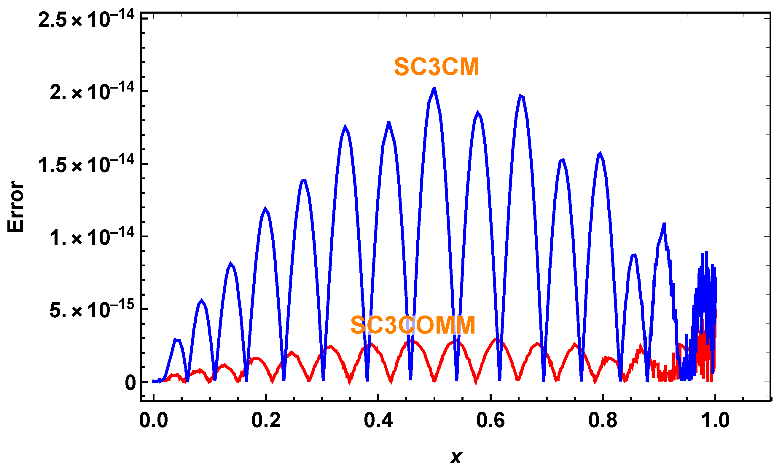
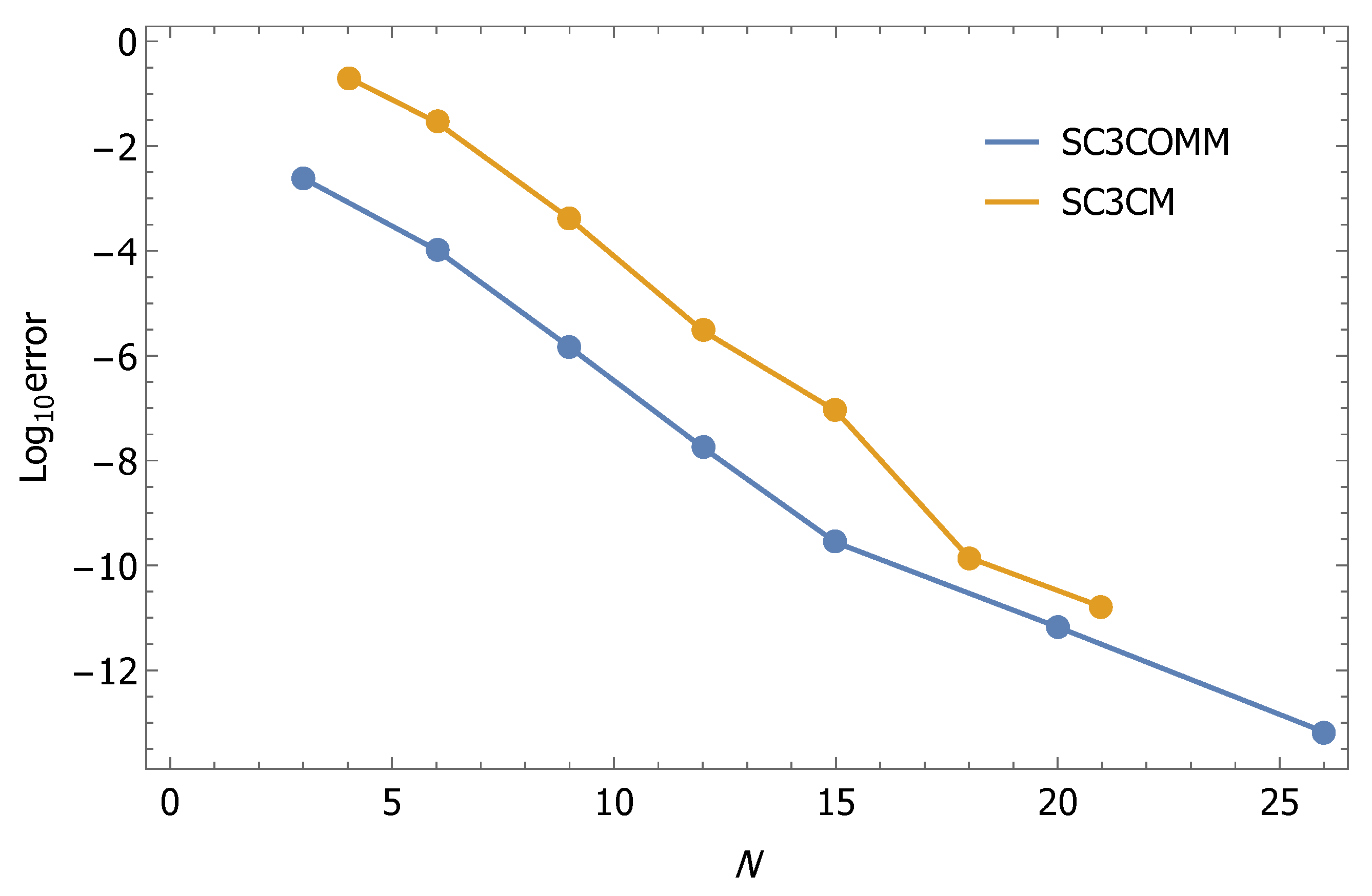
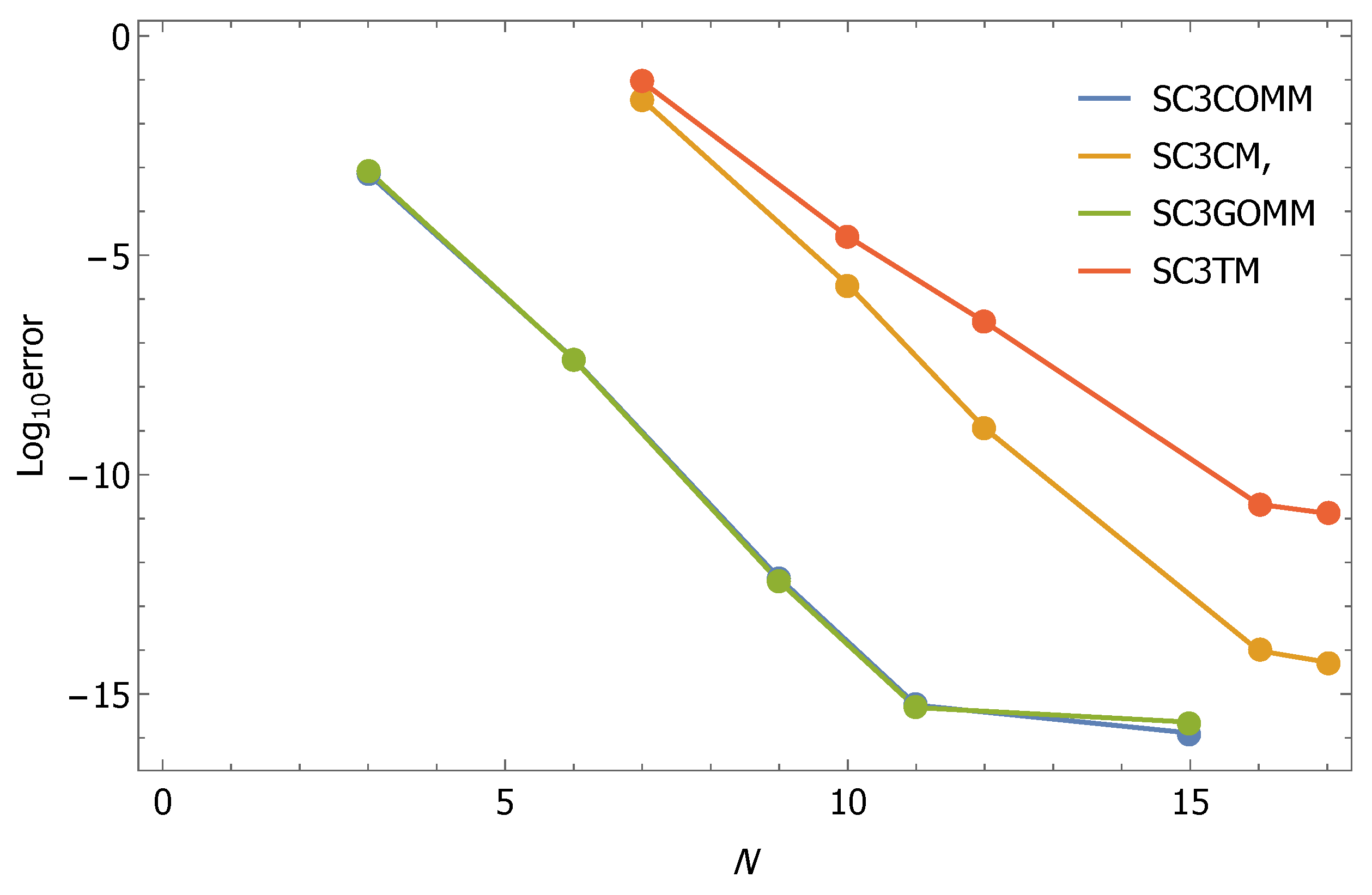
7. Numerical Results

This section focuses on providing some examples to demonstrate how easily our suggested techniques can be used. Additionally, some comparisons with several other approaches are provided.

Example 1.

Consider the non-linear Emden–Flower-type Equation (32), for the special case of $(p=2,q=1,k=3)$ [11,44,45]

$$u^{‴}\left(x\right)+{\displaystyle \frac{6}{x}}{u}^{″}\left(x\right)+{\displaystyle \frac{6}{x^2}}{u}^{\prime }\left(x\right)=6(x^6+2x^3+10)e^{-3u\left(x\right)},0\le x\le 1,$$

(50)

subject to the initial conditions

$$u\left(0\right)=0,u^{\prime }\left(0\right)=0,u^{″}\left(0\right)=0.$$

The exact solution of (50) is $u\left(x\right)=ln(1+x^3).$

Table 1 shows the maximum errors that our method SC3COMM might produce, whereas Table 2 compares our technique to the following methods:

• B-spline collocation method (BSCM) developed in [11].
• Varitional itereration method (VIM) in [44].
• Quartic B-spline method (QBSM) in [45].

Additionally, Figure 1 displays a comparison between the obtained error using the two presented methods, SC3COMM and SC3CM.

Table 1. Maximum absolute error of Example 1.

N	SC3COMM	SC3CM
6	$2.04719\times {10}^{-5}$	$1.19833\times {10}^{-3}$
9	$5.30930\times {10}^{-8}$	$2.04719\times {10}^{-5}$
15	$7.59007\times {10}^{-12}$	$2.22160\times {10}^{-9}$
21	$5.52367\times {10}^{-15}$	$4.62410\times {10}^{-13}$
22	$4.54192\times {10}^{-15}$	$9.12330\times {10}^{-14}$

Table 1. Maximum absolute error of Example 1.

N	SC3COMM	SC3CM
6	$2.04719\times {10}^{-5}$	$1.19833\times {10}^{-3}$
9	$5.30930\times {10}^{-8}$	$2.04719\times {10}^{-5}$
15	$7.59007\times {10}^{-12}$	$2.22160\times {10}^{-9}$
21	$5.52367\times {10}^{-15}$	$4.62410\times {10}^{-13}$
22	$4.54192\times {10}^{-15}$	$9.12330\times {10}^{-14}$

Table 2. Comparison between different methods of Example 1.

SC3COMM $(\mathit{N}=\mathbf{22})$	SC3CM $(\mathit{N}=\mathbf{22})$	VIM [44]	QBSM [45]	BSCM [11]
$4.542\times {10}^{-15}$	$2.123\times {10}^{-14}$	$1.10\times {10}^{-1}$	$1.29\times {10}^{-5}$	$4.08\times {10}^{-7}$

Table 2. Comparison between different methods of Example 1.

SC3COMM $(\mathit{N}=\mathbf{22})$	SC3CM $(\mathit{N}=\mathbf{22})$	VIM [44]	QBSM [45]	BSCM [11]
$4.542\times {10}^{-15}$	$2.123\times {10}^{-14}$	$1.10\times {10}^{-1}$	$1.29\times {10}^{-5}$	$4.08\times {10}^{-7}$

Example 2.

Consider the nonlinear Emden–Flower-type Equation (32), for the special case of $(p=2,q=2,k=4)$ [14,15]

$$u^{\left(4\right)}\left(x\right)+{\displaystyle \frac{8}{x}}{u}^{\left(3\right)}\left(x\right)+{\displaystyle \frac{12}{x^2}}{u}^{\left(2\right)}\left(x\right)+u^m\left(x\right)=0,0\le x\le 1,$$

(51)

subject to the initial conditions

$$u\left(0\right)=1,u^{\left(i\right)}\left(0\right)=0,i=1,2,3.$$

The exact solution of (51) is $u\left(x\right)=1-{\displaystyle \frac{x^4}{360}}$, for $m=0$.

The use of our two suggested techniques $SC3GOMM$ and $SC3COMM$ for $N=0,1,2,\dots$, gives the follwoing approximate solution: ${\displaystyle \widetilde{u_N}\left(x\right)=\sum _{i=0}^N{a}_i{\varphi }_i\left(x\right)}$, where $a_0=-{\displaystyle \frac{1}{360}}$ and $a_i=0,$$i=1,2,\dots ,N$. In view of (34), we obtain $u_N\left(x\right)=1-{\displaystyle \frac{x^4}{360}}$, which is the exact solution. Additionally, the application of two proposed methods $SC3TM$ and $SC3CM$ for $N=4,5,6,\dots$, gives ${\displaystyle u_N\left(x\right)=\sum _{i=0}^N{a}_i{V}_i^{*}\left(x\right)}$, where $a_0={\displaystyle \frac{5113}{5120}},a_1={\displaystyle \frac{-7}{7680}},a_2={\displaystyle \frac{-1}{2560}},a_3={\displaystyle \frac{-1}{10240}},$ $a_4={\displaystyle \frac{-1}{92160}}$, and $a_i=0,i=5,6,7,...,N$.

Example 3.

Consider the nonlinear Emden–Flower-type Equation (32), for the special case of $(p=3,q=1,k=4)$ [14,15]

$$u^{\left(4\right)}\left(x\right)+{\displaystyle \frac{12}{x}}{u}^{\left(3\right)}\left(x\right)+{\displaystyle \frac{36}{x^2}}{u}^{\left(2\right)}\left(x\right)+{\displaystyle \frac{24}{x^3}}{u}^{\left(1\right)}\left(x\right)+60(7-18x^4+3x^8)u^9\left(x\right)=0,0\le x\le 1,$$

(52)

subject to the boundary conditions

$$u\left(0\right)=1,u^{\left(i\right)}\left(0\right)=0,i=1,2,3.$$

The exact solution of (52) is $u\left(x\right)={\displaystyle \frac{1}{\sqrt{x^4+1}}}$.

The maximum errors introduced by applying our suggested method SC3COMM for various values of specific parameters N are shown in Table 3, while Table 4 compares the results obtained from our algorithm with the following two methods:

• The Adomian decomposition method (ADM) that is applied in [14].
• The reproducing kernel Hilbert space method (RKHSM) that is derived in [15].

Additionally, Figure 2 displays the Log-error for different N to demonstrate the stability of the solutions to Example 3 if the two methods SC3COMM and SC3CM are employed, respectively.

Table 3. Maximum absolute error of Example 3.

N	SC3COMM	SC3CM
6	$1.046\times {10}^{-4}$	$2.284\times {10}^{-2}$
9	$1.459\times {10}^{-6}$	$4.187\times {10}^{-4}$
15	$2.740\times {10}^{-10}$	$8.886\times {10}^{-8}$
21	$5.664\times {10}^{-12}$	$1.606\times {10}^{-11}$
26	$6.664\times {10}^{-14}$	$1.012\times {10}^{-11}$

Table 3. Maximum absolute error of Example 3.

N	SC3COMM	SC3CM
6	$1.046\times {10}^{-4}$	$2.284\times {10}^{-2}$
9	$1.459\times {10}^{-6}$	$4.187\times {10}^{-4}$
15	$2.740\times {10}^{-10}$	$8.886\times {10}^{-8}$
21	$5.664\times {10}^{-12}$	$1.606\times {10}^{-11}$
26	$6.664\times {10}^{-14}$	$1.012\times {10}^{-11}$

Table 4. Comparison between different methods of Example 3.

SC3COMM $(\mathit{N}=\mathbf{26})$	SC3CM $(\mathit{N}=\mathbf{21})$	RKHSM [15]	ADM [14]
$6.664\times {10}^{-14}$	$1.606\times {10}^{-11}$	$1.23016\times {10}^{-6}$	$5.21075\times {10}^{-5}$

Table 4. Comparison between different methods of Example 3.

SC3COMM $(\mathit{N}=\mathbf{26})$	SC3CM $(\mathit{N}=\mathbf{21})$	RKHSM [15]	ADM [14]
$6.664\times {10}^{-14}$	$1.606\times {10}^{-11}$	$1.23016\times {10}^{-6}$	$5.21075\times {10}^{-5}$

Example 4.

Consider the following nonlinear Emden–Flower-type Equation (32), for the special case of $(p=3,q=1,k=1)$ [14,15,46]

$$u^{\left(4\right)}\left(x\right)+{\displaystyle \frac{3}{x}}{u}^{\left(3\right)}\left(x\right)-96(1-10x^4+5x^8)e^{-4u}=0,0\le x\le 1,$$

(53)

subject to the boundary conditions

$$u^{\left(i\right)}\left(0\right)=0,i=0,1,2,3.$$

The exact solution of (53) is $u\left(x\right)=ln(1+x^4).$

The maximum errors produced by applying our two approaches, $SC3COMM$ and $SC3CM$, are shown in Table 5, and Table 6 compares these two methods to the following methods:

• The Adomian decomposition method (ADM) that applied in [14].
• The reproducing kernel Hilbert space method (RKHSM) that derived in [15].
• The Quartic B-spline method (QBSM) that developed in [46].

Table 5. Maximum absolute errors of Example 4.

N	SC3COMM	SC3CM
6	$9.323\times {10}^{-5}$	$9.030\times {10}^{-2}$
13	$6.421\times {10}^{-9}$	$4.312\times {10}^{-6}$
17	$2.370\times {10}^{-10}$	$6.421\times {10}^{-9}$
22	$1.512\times {10}^{-5}$	$7.179\times {10}^{-13}$

Table 5. Maximum absolute errors of Example 4.

N	SC3COMM	SC3CM
6	$9.323\times {10}^{-5}$	$9.030\times {10}^{-2}$
13	$6.421\times {10}^{-9}$	$4.312\times {10}^{-6}$
17	$2.370\times {10}^{-10}$	$6.421\times {10}^{-9}$
22	$1.512\times {10}^{-5}$	$7.179\times {10}^{-13}$

Table 6. Comparison between different methods of Example 4.

SC3COMM $(\mathit{N}=\mathbf{22})$	SC3CM $(\mathit{N}=\mathbf{22})$	RKHSM [15]	ADM [14]	QBSM [46]
$1.512\times {10}^{-13}$	$7.179\times {10}^{-11}$	$1.98579\times {10}^{-6}$	$7.56423\times {10}^{-5}$	$6.88\times {10}^{-7}$

Table 6. Comparison between different methods of Example 4.

SC3COMM $(\mathit{N}=\mathbf{22})$	SC3CM $(\mathit{N}=\mathbf{22})$	RKHSM [15]	ADM [14]	QBSM [46]
$1.512\times {10}^{-13}$	$7.179\times {10}^{-11}$	$1.98579\times {10}^{-6}$	$7.56423\times {10}^{-5}$	$6.88\times {10}^{-7}$

Example 5.

Consider the linear Emden–Flower-type Equation (32), for the special case of $(p=4,$$q=1,k=4)$

$$u^{\left(5\right)}+{\displaystyle \frac{16}{x}}{u}^{\left(4\right)}+{\displaystyle \frac{72}{x^2}}{u}^{\left(3\right)}+{\displaystyle \frac{96}{x^3}}{u}^{\left(2\right)}+{\displaystyle \frac{24}{x^4}}{u}^{\left(1\right)}-u=f\left(x\right),0\le x\le 1,$$

(54)

subject to the initial conditions

$$u^{\left(i\right)}\left(0\right)=0,i=0,1,2,3,4,$$

where $f\left(x\right)=(8400+9744x+3696x^2+592x^3+41x^4)e^x$. The exact solution of (54) is $u\left(x\right)=x^5{e}^x.$

Table 7. Maximum absolute error of Example 5.

N	SC3COMM	SC3GOMM	SC3CM	SC3TM
6	$4.373\times {10}^{-8}$	$4.249\times {10}^{-8}$	$1.863\times {10}^{-1}$	$1.910\times {10}^{-1}$
9	$4.362\times {10}^{-13}$	$3.672\times {10}^{-13}$	$9.633\times {10}^{-5}$	$2.019\times {10}^{-4}$
11	$5.450\times {10}^{-16}$	$4.926\times {10}^{-16}$	$4.373\times {10}^{-8}$	$6.944\times {10}^{-6}$
16	$1.671\times {10}^{-16}$	$1.221\times {10}^{-16}$	$9.710\times {10}^{-15}$	$2.163\times {10}^{-11}$

displays the maximum errors that resulted from the application of our four methods SC3COMM, SC3GOMM, SC3CM and SC3TM. Again, Figure 3 presents Log-error for various N to show the stability of solutions of Example 5 if the presented four methods are applied.

8. Results and Discussions

New spectral solutions to singular high-order type equations were presented in this paper. New types of modified Chebyshev polynomials of the third kind and their well-known classical types were used as basis functions. The core of the Galerkin matrix method that was designed in this paper for treating the high-order Emden–Fowler equations is based on the derivation of the first-order derivative of the modified Chebyshev polynomials in Theorem 1 and novel operational matrices of the derivatives of these modified polynomials in Corollary 2. The convergence analysis of the two proposed expansions is carefully investigated in Theorems 2 and 3. Numerical results in Section 7 show the efficiency and applicability of our algorithm. We think that the modified third-kind Chebyshev polynomials proposed in this paper could be used to handle diverse differential equations.

References

1. Lane, H.J. On the theoretical temperature of the sun, under the hypothesis of a gaseous mass maintaining its volume by its internal heat, and depending on the laws of gases as known to terrestrial experiment. Am. J. Sci. Arts 1870, 2, 57–74. [Google Scholar] [CrossRef] [Green Version]
2. Emden, R. Gaskugeln: Anwendungen der mechanischen Wärmetheorie auf kosmologische und meteorologische Probleme; Teubner: Leipzig, Germany, 1907. [Google Scholar]
3. Fowler, R.H. Further studies of Emden’s and similar differential equations. Q. J. Math. 1931, 1, 259–288. [Google Scholar] [CrossRef]
4. Singh, R.; Garg, H.; Guleria, V. Haar wavelet collocation method for Lane–Emden equations with Dirichlet,Neumann and Neumann–Robin boundary conditions. J. Compt. Appl. Math. 2019, 346, 150–161. [Google Scholar] [CrossRef]
5. Dizicheh, A.K.; Salahshour, S.; Ahmadian, A.; Baleanu, D. A novel algorithm based on the Legendre wavelets spectral technique for solving theLane–Emden equations. Appl. Numer. Math. 2020, 153, 443–456. [Google Scholar] [CrossRef]
6. Abd-Elhameed, W.M.; Ahmed, H.M. Tau and Galerkin operational matrices of derivatives for treating singular and Emden–Fowler third-order-type equations. Int. J. Mod. Phys. 2022, 33, 2250061. [Google Scholar] [CrossRef]
7. Abd-Elhameed, W.M. New Galerkin operational matrix of derivatives for solving Lane-Emden singular-type equations. Eur. Phys. J. Plus 2015, 130, 1–12. [Google Scholar] [CrossRef]
8. Wazwaz, A.M.; Rach, R.; Bougoffa, L.; Duan, J.S. Solving the Lane–Emden–Fowler type equations of higher orders by the Adomian decomposition method. CMES Comput. Model. Eng. Sci. 2014, 100, 507–529. [Google Scholar]
9. Hasan, Y.Q.; Zhu, L.M. Solving singular boundary value problems of higher-order ordinary differential equations by modified Adomian decomposition method. Commun. Nonlinear Sci. Numer. Simul. 2009, 14, 2592–2596. [Google Scholar] [CrossRef]
10. Kim, W.; Chun, C. A modified Adomian decomposition method for solving higher-order singular boundary value problems. Z. Für Naturforschung A 2010, 65, 1093–1100. [Google Scholar] [CrossRef]
11. Iqbal, M.K.; Abbas, M.; Wasim, I. New cubic B-spline approximation for solving third order Emden–Flower type equations. Appl. Math. Comput. 2018, 331, 319–333. [Google Scholar] [CrossRef]
12. Roul, P.; Thula, K. A fourth-order B-spline collocation method and its error analysis for Bratu-type and Lane–Emden problems. Int. J. Comput. Math. 2019, 96, 85–104. [Google Scholar] [CrossRef]
13. Wazwaz, A.M. The variational iteration method for solving systems of third-order Emden-Fowler type equations. J. Math. Chem. 2017, 55, 799–817. [Google Scholar] [CrossRef]
14. Wazwaz, A.M.; Rach, R.; Duan, J.S. Solving new fourth–order Emden–Fowler-type equations by the Adomian decomposition method. Int. J. Comput. Methods Eng. Sci. 2015, 16, 121–131. [Google Scholar] [CrossRef]
15. Dezhbord, A.; Lotfi, T.; Mahdiani, K. A numerical approach for solving the high-order nonlinear singular Emden–Fowler type equations. Adv. Differ. Equ. 2018, 2018, 161. [Google Scholar] [CrossRef]
16. Madduri, H.; Roul, P. A fast-converging iterative scheme for solving a system of Lane–Emden equations arising in catalytic diffusion reactions. J. Math. Chem. 2019, 57, 570–582. [Google Scholar] [CrossRef]
17. Canuto, C.; Hussaini, M.Y.; Quarteroni, A.; Zang, T.A. Spectral Methods in Fluid Dynamics; Springer: Berlin/Heidelberg, Germany, 1988. [Google Scholar]
18. Hesthaven, J.; Gottlieb, S.; Gottlieb, D. Spectral Methods for Time-Dependent Problems; Cambridge University Press: Cambridge, UK, 2007; Volume 21. [Google Scholar]
19. Boyd, J.P. Chebyshev and Fourier Spectral Methods; Courier Corporation: Chelmsford, MA, USA, 2001. [Google Scholar]
20. Trefethen, L.N. Spectral Methods in MATLAB; SIAM: Philadelphia, PA, USA, 2000; Volume 10. [Google Scholar]
21. Ahmed, H.M. Numerical solutions of Korteweg-de Vries and Korteweg-de Vries-Burger’s equations in a Bernstein polynomial basis. Mediterr. J. Math. 2019, 16, 102. [Google Scholar] [CrossRef]
22. Abd-Elhameed, W.M.; Alkenedri, A.M. Spectral solutions of linear and nonlinear BVPs using certain Jacobi polynomials generalizing third-and fourth-kinds of Chebyshev polynomials. CMES Comput. Model. Eng. Sci. 2021, 126, 955–989. [Google Scholar] [CrossRef]
23. Napoli, A.; Abd-Elhameed, W.M. An innovative harmonic numbers operational matrix method for solving initial value problems. Calcolo 2017, 54, 57–76. [Google Scholar] [CrossRef]
24. Doha, E.H.; Abd-Elhameed, W.M.; Bhrawy, A.H. New spectral-Galerkin algorithms for direct solution of high even-order differential equations using symmetric generalized Jacobi polynomials. Collect. Math. 2013, 64, 373–394. [Google Scholar] [CrossRef]
25. Abdelhakem, M.; Alaa-Eldeen, T.; Baleanu, D.; Alshehri, M.G.; El-Kady, M. Approximating real-life BVPs via Chebyshev polynomials’ first derivative pseudo-Galerkin method. Fractal Frac. 2021, 5, 165. [Google Scholar] [CrossRef]
26. Doha, E.H.; Abd-Elhameed, W.M.; Bassuony, M.A. On using third and fourth kinds Chebyshev operational matrices for solving Lane-Emden type equations. Rom. J. Phys 2015, 60, 281–292. [Google Scholar]
27. Doha, E.H.; Abd-Elhameed, W.M.; Bassuony, M.A. On the coefficients of differentiated expansions and derivatives of Chebyshev polynomials of the third and fourth kinds. Acta Math. Sci. 2015, 35, 326–338. [Google Scholar] [CrossRef]
28. Alsuyuti, M.M.; Doha, E.H.; Ezz-Eldien, S.S.; Bayoumi, B.I.; Baleanu, D. Modified Galerkin algorithm for solving multitype fractional differential equations. Math. Methods Appl. Sci. 2019, 42, 1389–1412. [Google Scholar] [CrossRef]
29. Abd-Elhameed, W.M. Novel expressions for the derivatives of sixth-kind Chebyshev polynomials: Spectral solution of the non-linear one-dimensional Burgers’ equation. Fractal Fract. 2021, 5, 53. [Google Scholar] [CrossRef]
30. Tu, H.; Wang, Y.; Lan, Q.; Liu, W.; Xiao, W.; Ma, S. A Chebyshev-Tau spectral method for normal modes of underwater sound propagation with a layered marine environment. J. Sound Vib. 2021, 492, 115784. [Google Scholar] [CrossRef]
31. Mokhtary, P.; Ghoreishi, F.; Srivastava, H.M. The Müntz-Legendre Tau method for fractional differential equations. Appl. Math. Model. 2016, 40, 671–684. [Google Scholar] [CrossRef]
32. Mohebbi, A. Crank–Nicolson and Legendre spectral collocation methods for a partial integro-differential equation with a singular kernel. J. Comput. Appl. Math. 2019, 349, 197–206. [Google Scholar] [CrossRef]
33. Çelik, I. Gegenbauer wavelet collocation method for the extended Fisher-Kolmogorov equation in two dimensions. Math. Methods Appl. Sci. 2020, 43, 5615–5628. [Google Scholar] [CrossRef]
34. Khader, M.M.; Adel, M. Numerical and theoretical treatment based on the compact finite difference and spectral collocation algorithms of the space fractional-order Fisher’s equation. Int. J. Mod. Phys. C 2020, 31, 2050122. [Google Scholar] [CrossRef]
35. Wang, F.; Zhao, Q.; Chen, Z.; Fan, C.M. Localized Chebyshev collocation method for solving elliptic partial differential equations in arbitrary 2D domains. Appl. Math. Comput. 2021, 397, 125903. [Google Scholar] [CrossRef]
36. Bansu, H.; Kumar, S. Numerical solution of space-time fractional Klein-Gordon equation by radial basis functions and Chebyshev polynomials. Inter. J. Appl. Comput. Math. 2021, 7, 1–19. [Google Scholar] [CrossRef]
37. Nouri, K.; Fahimi, M.; Torkzadeh, L.; Baleanu, D. Numerical method for pricing discretely monitored double barrier option by orthogonal projection method. AIMS Math. 2021, 6, 5750–5761. [Google Scholar] [CrossRef]
38. Sakran, M.R.A. Numerical solutions of integral and integro-differential equations using Chebyshev polynomials of the third kind. Appl. Math. Comp. 2019, 351, 66–82. [Google Scholar] [CrossRef]
39. Balaji, S.; Hariharan, G. An efficient operational matrix method for the numerical solutions of the fractional Bagley–Torvik equation using wavelets. J. Math. Chem. 2019, 57, 1885–1901. [Google Scholar] [CrossRef]
40. Loh, J.R.; Phang, C. Numerical solution of Fredholm fractional integro-differential equation with Right-sided Caputo’s derivative using Bernoulli polynomials operational matrix of fractional derivative. Mediterr. J. Math. 2019, 16, 28. [Google Scholar] [CrossRef]
41. Koepf, W. Hypergeometric Summation, 2nd ed.; Universitext Series; Springer: London, UK, 2014. [Google Scholar]
42. Andrews, G.E.; Askey, R.; Roy, R. Special Functions; Cambridge University Press: Cambridge, UK, 1999. [Google Scholar]
43. Stewart, J. Single Variable Essential Calculus: Early Transcendentals; Cengage Learning: Davis Drive Belmont, CA, USA, 2012. [Google Scholar]
44. Wazwaz, A.M. Solving two Emden-Fowler type equations of third order by the variational iteration method. Appl. Math. Inf. Sci. 2015, 9, 2429. [Google Scholar]
45. Mishra, H.K.; Saini, S. Quartic B-spline method for solving a singular singularly perturbed third-order boundary value problems. Am. J. Numer. Anal. 2015, 3, 18–24. [Google Scholar]
46. Iqbal, M.; Abbas, M.; Zafar, B. New Quartic B-spline approximations for numerical solution of fourth order singular boundary value problems. J. Math. 2020, 52, 47–63. [Google Scholar]
Figure 1. Comparison between the errors of Example 1 for N = 22 .
Axioms 12 00099 g001
Figure 2. Comparison between the errors of Example 3 for N = 3 , 4 , , 26 .
Axioms 12 00099 g002
Figure 3. Comparison between the errors of Example 5 for N = 3 , 4 , , 17 .
Axioms 12 00099 g003