Vibration of a Flexible Follower in a Cam Mechanism with Time-Dependent Boundary Effect

Abstract

A vibration analysis of a flexible follower in an oscillating follower cam system undergoing a rise-dwell-fall-dwell (RDFD) motion is performed. Owing to the time-dependent boundary effect caused by considering simultaneously the axial and the lateral displacements of the follower, two geometric constraints are formulated and added to Hamilton’s principle to establish the vibration equation of the motion of the follower. The coupled axial and lateral vibration of the flexible follower has been studied for the first time. The fast Fourier transform (FFT) spectrum generated from the time history is used for parametric studies. The numerical results of the present study show some new findings. The major spectral peaks for the lateral follower response locate at the low frequencies of 1 Ω, 3 Ω, 5 Ω, and 7 Ω and the high frequency near the fundamental natural frequency where Ω is the cam speed. The largest peak locates mostly at the frequency of 3 Ω. For the ascending and descending motions of the follower RDFD motion, three types of cam profiles are designed. Important new results are found: although the three cam profiles nearly overlap, the vibration results of the follower are quite different. By using a modified sinusoidal acceleration motion, the magnitude of the main lateral peak at low frequencies is minimized. The lateral peak amplitude near the fundamental natural frequency of the follower is the smallest when the cycloid displacement motion is adopted.

1. Introduction

Much work has been reported in cam mechanism research. In [1], the kinematics, dynamics, and design of the cam mechanism are presented. Osman et al. [2] considered the effect of clearance. The governing equations were established, taking into account the changes in displacement and velocity. The results showed that the bearing forces had an upper limit. Saka et al. [3] studied the effect of torsional vibrations on the camshaft’s mechanisms. Thanks to the reciprocating followers, the variable torque would make torsional vibrations on the camshaft. It was indicated that the torsional vibrations can affect the follower motion and the contact force. Yilmaz et al. [4] investigated the vibrations of a follower in the longitudinal direction. The follower with a constant cross section was considered. The partial differential equation was established by employing the Bernoulli method. The effect of internal damping was observed after the fourth eigen-frequency. Cveticanin [5] analyzed the motion stability of the driven cam system. Camshaft and follower flexibility were taken into account. The system-damping and nonlinear characteristics were also considered. The two-D.O.F. system was used to model the mechanism, including the system-damping and nonlinear characteristics. The stable conditions of the follower motion were analytically determined. Chang et al. [6] investigated the vibration of the follower of cam mechanisms for different cam profiles. A Rayleigh beam was used to model the flexible follower. The lateral deflection is expanded using the eigen-functions of a simply supported beam. The influence of parameters, including follower length, the radius of the cross section, and the total rise, was studied.

Sundar et al. [7] used a single-DOF system to model a rotating cam follower to study the contact dynamics. Point contact and line contact were considered to calculate the contact stiffness by using Hertzian contact theory. Hejma et al. [8] studied the construction of a cam mechanism. A coil spring was applied to press a flat-faced follower against a radial disk cam. A new cam profile was proposed with three known lifting functions. Yousuf [9] analyzed a roller follower and a polydyne cam with different cam speeds. The influence of the clearance of the follower guide on chaos was considered. Then Yousuf [10] modeled a spherical cam mechanism to study the nonlinear dynamics. The effect of parameters such as follower guide size and cam angular velocity was investigated. The follower aperiodic motion has also been discussed.

Yousuf [11] studied the effect of the internal distance of the guide rail from the interior, the constant rotational speed of the cam, and the offset of the follower on the chaos. Chang et al. [12] carried out theoretical research and experimental verification on the improved design of the assembled conjugate disk cam to achieve complete rotation balance. Based on the proposed theoretical study and experimental verification, the proposed modified design has been proven to be feasible and effective to improve the dynamic performance of the conjugate cam mechanism with oscillating roller followers. Wang and Wang [13] developed a novel surface-based vibration isolation mechanism for the parametric design of stiffness characteristics, which consisted of double links, coil springs, roller cam followers, and curved surfaces. This design approach was used to isolate severe vibrations. An experimental platform was also built, and a vibration test was carried out to verify the vibration isolation performance. Many researchers have performed the dynamic analysis of beam systems with the effects of time-dependent boundary [14,15,16,17,18,19,20]. Fung [21] analyzed the behavior of a slider-crank mechanism. The time-dependent boundary effects were considered in the modeling of the flexible linkage. For the vibration analysis of the quick-return mechanism, time-dependent boundary effects were also considered in the flexible link modeling [22,23]. Lowe et al. [24] investigated propagating waves generated by time-dependent traction boundary conditions in elastic structural elements. They reported solutions to generalized models of this important class of problems through the well-established Mindlin-Goodman method and its two successors. Chai et al. [25] studied the aerothermoelastic properties of composite laminates with time-dependent boundary conditions. The results showed that both the displacement feedback control and the linear quadratic Gaussian method can suppress the vibration. They [26] also studied the nonlinear vibration of composite laminates with time-dependent boundary conditions and base excitations. The results contributed to the nonlinear dynamic analysis and design of the studied panels. Chai et al. [27] investigated the aerothermoelastic flutter behavior of nonlinear composite laminates with time-dependent boundary conditions in supersonic airflow and studied the active flutter and aerothermal postbuckling suppression for the studied panels. It was shown that the developed linear quadratic regulator/extended Kalman filter controller was more effective in the flutter and postbuckling control of the studied panels.

Horssen et al. [28] showed how to use characteristic coordinates to solve initial boundary value problems for wave equations involving Robin-type boundary conditions with time-dependent coefficients. Akbari et al. [29] proposed a comprehensive analytical technique to evaluate the non-Fourier thermal behavior of 3D hollow spheres under arbitrarily chosen space- and time-dependent boundary conditions. A quantitative analysis, including the profiles of the time-dependent temperature and 3D distributions of temperature at different time frames, has been performed. Belekar et al. [30] presented an analytical solution for the temperature distribution in a stationary wet granular mixture in a heated cylindrical vessel, a typical geometry for an industrial filter-dryer. It provided useful predictions of the wall heat flux that was required as an input to zero-dimensional heat and mass transfer models to accurately predict the heating and drying time.

To the best of the author’s knowledge, the time-dependent boundary effect caused by the axial and lateral displacements of the follower has not been considered in the vibration analysis modeling of the oscillating roller follower. In this study, a dynamic analysis of a cam mechanism with an oscillating roller follower is performed. One end of the follower is connected with the roller rolling along the cam guide rail, and the other end of the follower rotates around the fixed pivot. The contact point between the roller and the cam is a time-dependent boundary condition of the follower. The axial and lateral deflections are simultaneously established for the vibration analysis of the flexible follower. In traditional research, the contact point between the roller and the cam can be calculated by using kinematics. To calculate the contact position, two time-dependent constraint equations are applied to the derivation of the motion equations, utilizing Hamilton’s principle. The author [6] has so far modeled the flexible follower with only lateral deflection, so the contact position can be determined using only kinematic analysis. In this study, the assumed modes are employed to establish the deflections. By applying the Runge–Kutta method to solve the system equations of motion, the follower deflections can be obtained. This results in the time history and FFT spectrum of the axial and lateral vibration response. The axial and lateral vibration analysis of the follower for three kinds of rise-dwell-fall-dwell motion is performed. The effects of system parameters such as the base circle radius of the cam, the rotational speed of the cam, the length of the follower, the radius of the cross section of the follower, the total rise of the follower, and the stiffness value of the torsion spring on vibration behavior are also studied.

The novelty and contributions of this paper are as follows:

(1)

The best novelty of the work is that the vibration modeling of an oscillating roller follower that factors in the time-dependent boundary effect caused by the axial and lateral displacements of follower has been proposed for the first time.

(2)

The proposed method combining Hamilton’s principle with Lagrangian multipliers, the assumed mode method, and the simplification of a differential-algebraic equation can effectively solve the follower vibration problem under consideration of time-dependent boundary conditions.

(3)

The axial and lateral vibration spectra of the follower for the three kinds of rise-dwell-fall-dwell motion, including the motion of cycloid displacement, modified sinusoidal acceleration, and modified trapezoidal acceleration, are obtained and discussed.

2. Derivation of System Equations of Motion

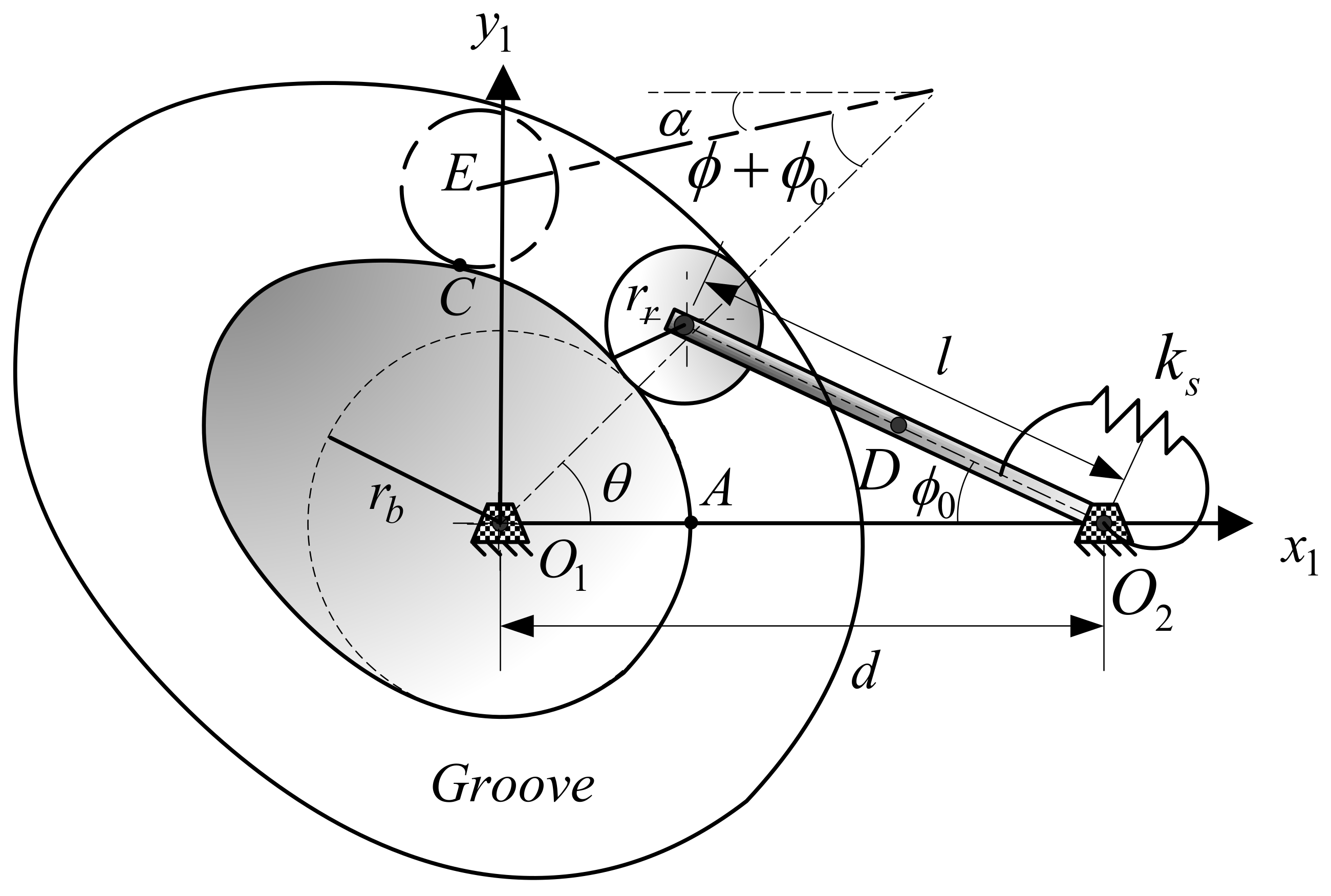
Figure 1 and Figure 2 show the schematic diagram of the oscillating roller-follower cam system. One end of the follower is connected with a roller rolling in the cam groove, and the other end of the follower is provided with a preloaded torsion spring and rotates around a fixed pivot ($O_2$). Rayleigh beam theory is used to model the follower. If the contact (C) between the roller and the cam is smooth, friction will be negligible. Next, the parameters in Figure 1 and Figure 2 are introduced. $d$ is the distance from the follower-fixed pivot to the center of the cam rotation ($O_1$), $l$ is the follower length, $r_b$ is the cam radius of the base circle, $r_r$ is the radius of the roller, $k_s$ is the stiffness of the torsion spring, E is the follower’s endpoint, P is any point of the follower, D is the output node, $\theta$ is the cam rotation angle, ${\phi }_o$ is the initial follower angle, and $\phi$ is the follower angular displacement. $O_1-x_1{y}_1$ is the rotating coordinate system fixed on the cam. A is a reference point of the cam profile and located on the $O_1-x_1$ axis, $O_1-XY$ is the fixed coordinate system, and $O_2-xy$ is a rotating coordinate system fixed on the follower. $u$ is the axial displacement along the x-axis, and $v$ is the lateral displacement along the y-axis. $\mathsf{\Omega }$ is the angular velocity of the cam, and $\varphi =\phi (\mathsf{\Omega }t)+{\phi }_o$.

Start by building the cam profile by using three different movements. Then using the derived time-dependent constraint equation, the work done by the constraint force is derived. The kinetic and strain energies of the system are formulated. The assumed mode method is applied to expand the follower displacements in the axial and lateral directions. According to Hamilton’s principle, the equations of the motion of the system can be derived by variation equations.

2.1. Establishment of the Cam Profile

Figure 1 shows the schematic diagram of the oscillating roller-follower cam system. The angular displacement of the follower is a function of the cam rotation angle $\theta$, denoted as $\phi (\theta )$. $\phi (\theta )=0$ at $\theta =0$. A vibration analysis of a follower with three kinds of the rise-dwell-fall-dwell motion (RDFD motion) of the oscillating follower is carried out, as shown in Figure 3. For the rise and fall cycles, three motions, such as the motion of cycloid displacement (CD), modified sinusoidal acceleration (MSA), and modified trapezoidal acceleration (MTA), are used to design the cam profile. The three motions that express the ascending function $\phi (\theta )$ are described as follows [1]:

• CD:

$$0\le \theta \le \beta : \phi (\theta )={\phi }_T\left(\frac{\theta }{\beta }-\frac{1}{2\pi }\sin (\frac{2\pi \theta }{\beta })\right)$$

(1)

2.

MSA:

$$0\le \theta \le \frac{\beta }{8}: \phi (\theta )={\phi }_T\left(\frac{\pi }{4+\pi }\frac{\theta }{\beta }-\frac{\pi }{4(4+\pi )}\sin (\frac{4\pi \theta }{\beta })\right)$$

$$\frac{\beta }{8}<\theta \le \frac{7\beta }{8}: \phi (\theta )={\phi }_T\left(\frac{2}{4+\pi }+\frac{\pi }{4+\pi }\frac{\theta }{\beta }-\frac{9}{4(4+\pi )}\cos (\frac{4\pi \theta }{3\beta }-\frac{\pi }{6})\right)$$

(2)

$$\frac{7\beta }{8}<\theta \le \beta : \phi (\theta )={\phi }_T\left(\frac{4}{4+\pi }+\frac{\pi }{4+\pi }\frac{\theta }{\beta }-\frac{9}{4(4+\pi )}\sin (\frac{4\pi \theta }{\beta })\right)$$

3.

MTA:

$$0\le \theta \le \frac{\beta }{8}: \phi (\theta )={\phi }_T\left(0.38898448\frac{\theta }{\beta }-0.0309544 \sin (\frac{4\pi \theta }{\beta })\right)$$

$$\frac{\beta }{8}<\theta \le \frac{3\beta }{8}: \phi (\theta )={\phi }_T\left(2.44406{\left(\frac{\theta }{\beta }\right)}^2-0.22203097\frac{\theta }{\beta }+0.00723407\right)$$

$$\frac{3\beta }{8}<\theta \le \frac{\beta }{2}:\phi (\theta )={\phi }_T\left(1.6110154\frac{\theta }{\beta }-0.0309533\sin (\frac{4\pi \theta }{\beta }-\pi )-0.3055077\right)$$

(3)

$$\frac{\beta }{2}<\theta \le \frac{5\beta }{8}: \phi (\theta )={\phi }_T\left(1.6110154\frac{\theta }{\beta }+0.0309544\sin (\frac{4\pi \theta }{\beta })-0.3055077\right)$$

$$\frac{5\beta }{8}<\theta \le \frac{7\beta }{8}: \phi (\theta )={\phi }_T\left(-2.44406184{\left(\frac{\theta }{\beta }\right)}^2+4.6660917\frac{\theta }{\beta }-1.2292648\right)$$

$$\frac{7\beta }{8}<\theta \le \beta : \phi (\theta )={\phi }_T\left(0.6110154+0.38898448\frac{\theta }{\beta }+0.0309544\sin (\frac{4\pi \theta }{\beta }-\pi )\right)$$

In Equations (1)–(3), $\beta$ is the rising cycle, which is set as $\frac{\pi }{2}$ in this paper, and ${\phi }_T$ is the total rise range. The ascending function is suitable for descending, with minor modifications. To convert an ascending function to a descending function, simply subtract the ascending function $\phi (\theta )$ from the largest ascending ${\phi }_T$. The descending cycle is also set to $\frac{\pi }{2}$.

By using envelope theory [1], the cam profile can be determined. The cam contour coordinates are indicated as ($x_{1C}, y_{1C}$) and can be derived as follows (see Figure 1):

$$\begin{array}{l}{x}_{1C}=d\cos \theta -l\cos \alpha -\frac{r_r}{\sqrt{1+{(\frac{P}{Q})}^2}},\\ y_{1C}=d\sin \theta -l\sin \alpha +(x_{1C}-d\cos \theta +l\cos \alpha )\frac{P}{Q}\end{array}$$

(4)

where

$$\begin{array}{l}P=d\sin \theta -l(1-{\phi }^{\prime }(\theta ))\sin \alpha ,\\ Q=d\cos \theta -l(1-{\phi }^{\prime }(\theta ))\cos \alpha ,\\ \alpha =\theta -\phi (\theta )-{\phi }_0\end{array}$$

(5)

The roller center coordinate is indicated as ($x_{1E}, y_{1E}$) and can be derived as follows:

$$\begin{array}{l}{x}_{1E}=d\cos \theta -l\cos \alpha ,\\ y_{1E}=d\sin \theta -l\sin \alpha \end{array}$$

(6)

From the observation in Figure 1, it can be seen that the follower’s initial position before the start of the rise is ${\phi }_o$, and the derivation is as follows:

$${\phi }_o={\cos }^{-1}\hspace{0.33em}\frac{d^2+l^2-{(r_b+r_r)}^2}{2d l}$$

(7)

2.2. The Constraints of the Time-Dependent Boundary

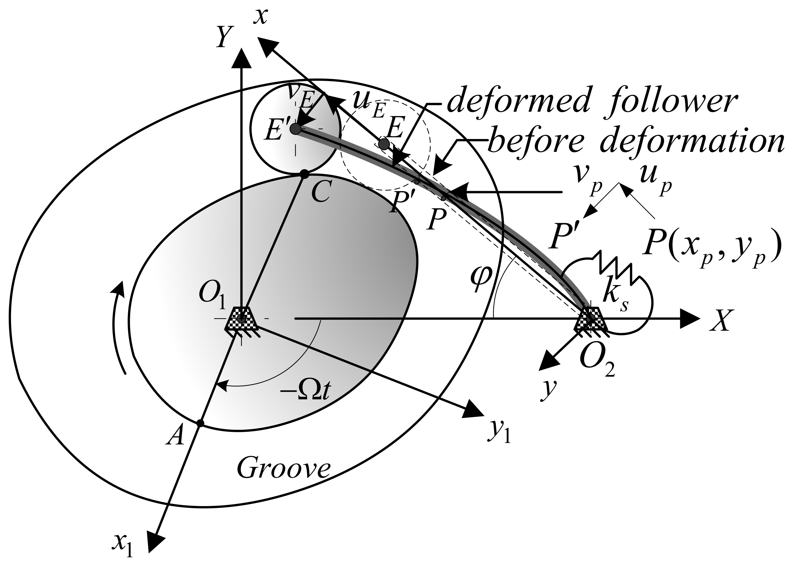
Figure 2 shows the deformation diagram of the cam system. The angular velocity of the cam is constant and is given as $\mathsf{\Omega }$. $O_1-x_1{y}_1$ is the rotating coordinate system fixed on the cam. $O_1-XY$ is the fixed coordinate system, and the corresponding unit coordinate vector is given as ${\{I,J\}}^T$. The point $E^{\prime }$ is the deformed follower’s endpoint, and the point C is the contact point between the roller and the cam. The points $E^{\prime }$ and C expressed in the fixed frame are given as follows:

$$\begin{array}{l}{X}_{E^{\prime }}=x_{1E^{\prime }}\cos \mathsf{\Omega }t+y_{1E^{\prime }}\sin \mathsf{\Omega }t,\hspace{1em}\\ Y_{E^{\prime }}=-x_{1E^{\prime }}\sin \mathsf{\Omega }t+y_{1E^{\prime }}\cos \mathsf{\Omega }t,\\ X_C=x_{1C}\cos \mathsf{\Omega }t+y_{1C}\sin \mathsf{\Omega }t,\hspace{1em}\\ Y_C=-x_{1C}\sin \mathsf{\Omega }t+y_{1C}\cos \mathsf{\Omega }t\end{array}$$

(8)

Figure 2 shows the deformation diagram of the cam system. $O_2-xy$ is a rotating coordinate system: its unit coordinate vector is ${\{i,j\}}^T$, and its x-axis is coincident with the follower’s undeformed centerline. After the deformation of the follower, the follower’s endpoint E moves to the position $E^{\prime }$ by axial displacement $u_E$ along the x-axis and lateral displacement $v_E$ along the y-axis. It is the time-dependent boundary at one end of the follower. The deformed position vector of E relative to the origin $O_1$ can be represented as follows:

$$\begin{array}{ll}{R}_{E^{\prime }}& =dI+(l+u_E)i+v_{E}j\\ & =[d-(l+u_E)\cos \varphi -v_E\sin \varphi ]I\\ & \hspace{1em}+[(l+u_E)\sin \varphi -v_E\cos \varphi ]J\end{array}$$

(9)

where $\varphi =\phi (\mathsf{\Omega }t)+{\phi }_o$ is the rise angle of the follower at time t.

By combining Equations (8) and (9), the two geometric constraints along the X and Y axes can be obtained, as follows:

$${\mathsf{\Phi }}_1=d-(l+u_E)\cos \varphi -v_E\sin \varphi -X_{E^{\prime }}=0$$

(10)

$${\mathsf{\Phi }}_2=(l+u_E)\sin \varphi -v_E\cos \varphi -Y_{E^{\prime }}=0$$

(11)

In Equations (10) and (11), $\varphi (\mathsf{\Omega }t)$, $u_E$, and $v_E$ simultaneously occur. This can be interpreted as the coupling of rigid body rotation and flexible vibration under the time-dependent boundaries.

2.3. The Strain Energy, Potential Energy, and Kinetic Energy

2.3.1. The Strain Energy

After the follower is deformed, any point P of the follower moves to position $P^{\prime }$ with axial displacement $u_p$ along the x-axis and lateral displacement $v_p$ along the y-axis, as shown in Figure 2. By ignoring higher-order terms when applying Lagrangian strain, the follower strain can be derived, as follows:

$$\begin{array}{ll}{\epsilon }_{xx}& =\frac{\partial u_p}{\partial x }-y\frac{{\partial }^2{v}_p}{\partial x^2}+\frac{1}{2}[{(\frac{\partial u_p}{\partial x }-y\frac{{\partial }^2{v}_p}{\partial x^2})}^2+{(\frac{\partial v_p}{\partial x})}^2]\\ & \approx \frac{\partial u_p}{\partial x }-y\frac{{\partial }^2{v}_p}{\partial x^2},\\ {\epsilon }_{yy}& =\frac{1}{2}{(\frac{\partial v_p}{\partial x})}^2\approx 0, \hspace{0.33em}\\ {\epsilon }_{xy}& =\frac{1}{2}[\frac{\partial v_p}{\partial x}-\frac{\partial v_p}{\partial x}-\frac{\partial v_p}{\partial x}(\frac{\partial u_p}{\partial x }-y\frac{{\partial }^2{v}_p}{\partial x^2})]\approx 0\end{array}$$

(12)

where $\epsilon$ is the strain at the point P of the follower.

By using Hooke’s law, the follower strain energy is

$$\begin{array}{ll}{U}_{rod}& =\frac{1}{2}{\displaystyle \underset{V}{\iiint }E {(\frac{\partial u_p}{\partial x }-y \frac{{\partial }^2{v}_p}{\partial x^2})}^2} dV\\ & =\frac{1}{2}[E A {(\frac{\partial u_p}{\partial x })}^2+E I {(\frac{{\partial }^2{v}_p}{\partial x^2})}^2]dx\end{array}$$

(13)

where $E$, $A$, and $I$ are the material elasticity modulus, the cross-sectional area, and moment of inertia of the cross-sectional area of the follower, respectively. Additionally, the cross section of the follower is designated as a circle, so $A=\pi r_f{}^2$ and $I=\frac{\pi r_f{}^4}{4}$, where $r_f$ is the radius of the circular cross section of the follower.

Given the deformation of the torsion spring, the corresponding strain energy is given as

$$U_s=\frac{1}{2}{k}_s{(\varphi -{\phi }_{se})}^2$$

(14)

where $k_s$ is the stiffness of the torsion spring, $\varphi =\phi (\mathsf{\Omega }t)+{\phi }_o$, and ${\phi }_{se}={\phi }_o-{\phi }_p$. Additionally, ${\phi }_{se}$ is the static equilibrium angle of the torsion spring, and ${\phi }_p$ is the preload angle of the torsion spring.

2.3.2. The Potential Energy

The position vector of the position $P^{\prime }$ shown in Figure 2 is

$$R_{P^{\prime }}=(x_p+u_p-y_p \frac{\partial v_p}{\partial x}) i+(y_p+v_p) j$$

(15)

Although the effect in this study may be small, the gravitational potential energy $V$, including the rod component $V_{rod}$ and the roller component $V_{roller}$, is derived as follows:

$$\begin{array}{ll}V& =V_{rod}+V_{roller}\\ & =\frac{1}{2}{\displaystyle \underset{V}{\iiint } R_{P^{\prime }}\cdot J} \rho g dV+ R_{E^{\prime }}\cdot J m_r g\\ & ={\displaystyle {\int }_{ 0}^{ l} }[(x_p+u_p)\sin \varphi -v_p\cos \varphi ] \rho gAdx+ [(l+u_E)\sin \phi -v_E\cos \phi ] m_r g\end{array}$$

(16)

where $\rho$ is the mass density, $g$ is gravitational acceleration, and $m_r$ is the roller’s mass.

2.3.3. The Kinetic Energy

The velocity at position $P^{\prime }$ can be derived by taking the derivative of position vector $R_{P^{\prime }}$ with respect to time t, as follows:

$${\dot{R}}_{P^{\prime }} =[{\dot{u}}_p-y_p \frac{\partial {\dot{v}}_p}{\partial x}+\dot{\varphi } (y_p+v_p)]i+[{\dot{v}}_p-\dot{\varphi } (x_p+u_p-y_p \frac{\partial v_p}{\partial x})]j$$

(17)

By integrating the following, the kinetic energy of a follower rod is

$$\begin{array}{ll}{T}_{rod}& =\frac{1}{2}{\displaystyle \underset{V}{\iiint }\rho }{‖{\dot{R}}_{P^{\prime }}‖}^2 dV\\ & =\frac{1}{2}{\displaystyle {\int }_{ 0}^{ l}\{}\rho A [{\dot{u}}_p{}^2+{\dot{\varphi }}^2 v_p{}^2+2\dot{\varphi } {\dot{u}}_p v_p+{\dot{v}}_p{}^2+{\dot{\varphi }}^2{(x_p+u_p)}^2\\ & -2\dot{\varphi } {\dot{v}}_p (x_p+u_p)]+\rho I [{(\frac{\partial {\dot{v}}_p}{\partial x})}^2+{\dot{\varphi }}^2+{\dot{\varphi }}^2{(\frac{\partial v_p}{\partial x})}^2-2\dot{\varphi }\frac{\partial {\dot{v}}_p}{\partial x}]\}dx\end{array}$$

(18)

The translational energy and rotational energy of the roller are as below:

$$\begin{array}{ll}{T}_{roller}& =\frac{1}{2}{m}_r {‖{\dot{R}}_{E^{\prime }}‖}^2+\frac{1}{2}{J}_r{\dot{\theta }}_r^2\\ & =\frac{1}{2}{m}_r\{{({\dot{u}}_E+\dot{\varphi } v_E)}^2+{[\dot{\varphi } (l+u_E)-{\dot{v}}_E]}^2\}\\ & \hspace{1em}+\frac{1}{2}\frac{J_r}{r_r^2} [{({\dot{X}}_{E^{\prime }}-{\dot{X}}_C)}^2+{({\dot{Y}}_{E^{\prime }}-{\dot{Y}}_C)}^2]\end{array}$$

(19)

where $J_r$ is the roller’s mass polar moment of inertia and ${\theta }_r$ is the roller’s rotation angle.

2.4. Assumed Mode Method

The follower rotates about a fixed pivot. To satisfy the hinged boundary, the following assumed mode method [31] is applied to expand the axial and lateral displacements at the point P:

$$u_p(x_p,t)=a_{u1}(t) \frac{x_p}{l}+{\displaystyle \sum _{i=2}^N{a}_{ui}(t)\sin \frac{(i-1) \pi x_p}{l}}$$

(20)

$$v_p(x_p,t)=a_{v1}(t) \frac{x_p}{l}+{\displaystyle \sum _{i=2}^N{a}_{vi}(t)\sin \frac{(i-1) \pi x_p}{l}}$$

(21)

where $\frac{x_p}{l}$ is the first mode satisfying the displacement of the follower endpoint connected to the roller. The other modes use $\sin \frac{(i-1) \pi x_p}{l}$, $i=2,\hspace{0.33em}3,\hspace{0.33em}\cdots$. $a_{ui}(t)$ and $a_{vi}(t)$ are the corresponding amplitudes of axial and lateral displacements $u_p$ and $v_p$.

2.5. Hamilton’s Principle

By applying the variational principle (Hamilton’s principle) to the follower system under study, the following equation is obtained:

$${\displaystyle {\int }_{ t_1}^{ t_2}\delta [(}{T}_{rod}+T_{roller})-(U_{rod}+U_s)-(V_{rod}+V_{roller})+{\lambda }_1{\mathrm{\Phi }}_1+{\lambda }_2{\mathrm{\Phi }}_2 ]dt=0$$

(22)

In this formula, the kinetic energy, strain energy, and potential energy are used, and the virtual work caused by the time-dependent geometric constraints is also included by applying the Lagrange multiplier.

By expanding the displacements in Equation (22) by using the assumed modes in Equations (20) and (21), the system equation of motion in vector form is established below.

$$M \ddot{Q}+N+{\Phi }_Q^T \lambda =F$$

(23)

where $M$ and $\Phi$ are the mass matrix and constraint vector, respectively, which are functions of the generalized coordinate vector $Q$. The dynamic vector $N$ is a function of $Q$ and $\dot{Q}$. The damping and Coriolis effects are present in this vector. The vector $F$ on the right side of the equation is caused by gravity.

The constraint vector $\Phi$ formed by the combination of Equations (10) and (11) is given as

$$\Phi =[\begin{array}{cc}{\mathrm{\Phi }}_1& {\mathrm{\Phi }}_2\end{array}]{ }^T=0$$

(24)

The vector $Q$ is shown below:

$$Q=[\begin{array}{ccccccccc}{a}_1& a_2& a_3 \cdots & a_N& b_1& b_2& b_3 \cdots & b_N& \theta \end{array}],$$

(25)

By taking the time derivative of Equation (24) twice, the constraint acceleration equation is obtained as follows:

$${\Phi }_Q \ddot{Q}=-[{({\Phi }_Q \dot{Q})}_Q +2\frac{\partial {\Phi }_Q}{\partial t}] \dot{Q}-\frac{{\partial }^2\Phi }{\partial t^2}\equiv \xi$$

(26)

By combining Equations (23) and (26), the equation of motion of the system is

$$\left[\begin{array}{cc}M& {\Phi }_Q^T\\ {\Phi }_Q& 0\end{array}\right]\left[\begin{array}{c}\ddot{Q}\\ \lambda \end{array}\right]=\left[\begin{array}{c}F-N\\ \xi \end{array}\right]$$

(27)

The follower vibration of the studied cam system can be analyzed by solving the above differential-algebraic equation.

3. Simplification of Differential-Algebraic Equation

The vector $Q$ is divided into the following by applying the partitioning method [32]:

$$Q=[{\begin{array}{cc}{q}_1& q\end{array}}_2]$$

(28)

where

$$q_1=[\begin{array}{cccccccc}{a}_1& a_2& \cdots & a_N& b_1& b_2& \cdots & b_{N-1}\end{array}],$$

(29)

$$q_2=[\begin{array}{cc}{b}_N& \theta \end{array}]$$

(30)

Substituting the decomposition of Equation (28) into Equation (27), the equation of motion for the system is expressed as

$$\begin{array}{l}{M}^{pp}{\ddot{q}}_1+M^{pq}{\ddot{q}}_2+{\Phi }_{q_1}^T\lambda =F^{q_1}-N^{q_1}\\ M^{qp}{\ddot{q}}_1+M^{qq}{\ddot{q}}_2+{\Phi }_{q_2}^T\lambda =F^{q_1}-N^{q_2}\\ {\Phi }_p^{}{\ddot{q}}_1+{\Phi }_q^{}{\ddot{q}}_2=\xi \end{array}$$

(31)

By simplifying Equation (31) by eliminating $\lambda$ and ${\ddot{q}}_2$, the equation becomes

$$\tilde{M}(q_1) {\ddot{q}}_1+\tilde{N}(q_1, \hspace{0.33em}{\dot{q}}_1)=0$$

(32)

where

$$\begin{array}{ll}\tilde{M}& =M^{q_1{q}_1}-M^{q_1{q}_2}{\Phi }_{q_2}^{-1}{\Phi }_{q_1}-{\Phi }_{q_1}^T({\Phi }_{q_2}^{-1})(M^{q_2{q}_1}-M^{q_2{q}_2}{\Phi }_{q_2}^{-1}{\Phi }_{q_1}),\\ \tilde{N}& =[N^{q_1}-F^{q_1}-{\Phi }_{q_1}^T{({\Phi }_{q_2}^{-1})}^T(N^{q_2}-F^{q_2})]\\ & +[M^{q_1{q}_2}{\Phi }_{q_2}^{-1}-{\Phi }_{q_1}^T{({\Phi }_{q_2}^{-1})}^T{M}^{q_2{q}_2}{\Phi }_{q_2}^{-1} ] \xi \end{array}$$

(33)

Let

$${\rm B}={[q_1{\dot{q}}_1]}^T$$

(34)

Equation (32) is re-expressed as

$$\dot{B}=\left[\begin{array}{c}{\dot{q}}_1\\ -{\tilde{M}}^{-1}\tilde{N}\end{array}\right]$$

(35)

To study the vibration of the follower, the Runge–Kutta fourth-order method can be used to solve Equation (35).

4. Numerical Results and Discussion

By using a numerical example of a follower cam system, the vibration of a flexible follower is studied. The follower’s rise-dwell-fall-dwell motion (RDFD motion) is considered, as shown in Figure 3. Three motions, such as the motion of cycloid displacement (CD), modified sinusoidal acceleration (MSA), and modified trapezoidal acceleration (MTA), are used to design the cam profile for the ascending and descending cycles. The system parameter data of the studied cam mechanism for numerical analysis are shown in

Table 1. Data for the cam system parameters.

$A$	$78.54\hspace{0.33em}{\mathrm{mm}}^2$	$r_b$	$66 \hspace{0.33em}\mathrm{mm}$
$d$	$136 \hspace{0.33em}\mathrm{mm}$	$r_f$	$5\hspace{0.33em}\mathrm{mm}$
$E$	$2.1\times {10}^8\mathrm{kg}/\mathrm{mm}\cdot {\mathrm{s}}^2$	$r_r$	$15\hspace{0.33em}\mathrm{mm}$
$g$	$9810\hspace{0.33em} {\mathrm{mm}/\mathrm{s}}^2$	$\beta$	$\pi /2$
$I$	$490.87{\mathrm{mm}}^4$	$\rho$	$7.8\times {10}^{-6}{\mathrm{kg}/\mathrm{mm}}^3$
$J_r$	$5.625\hspace{0.33em}\mathrm{kg}\cdot {\mathrm{mm}}^2$	$\mathsf{\Omega }$	320 $\mathrm{rad}/\mathrm{s}$
$k_s$	$1.44\times {10}^5\mathrm{kg}\cdot {\mathrm{mm}}^2{/\mathrm{s}}^2$	${\phi }_p$	$\pi /90$
$l$	98$\mathrm{mm}$	${\phi }_T$	$\pi /18$
$m_r$	$0.05\hspace{0.33em}\mathrm{kg}$

. The vibration responses in the lateral and axial direction at the output node $D$ ($0.55l$ from $O_2$) of the follower, as shown in Figure 1, are investigated.

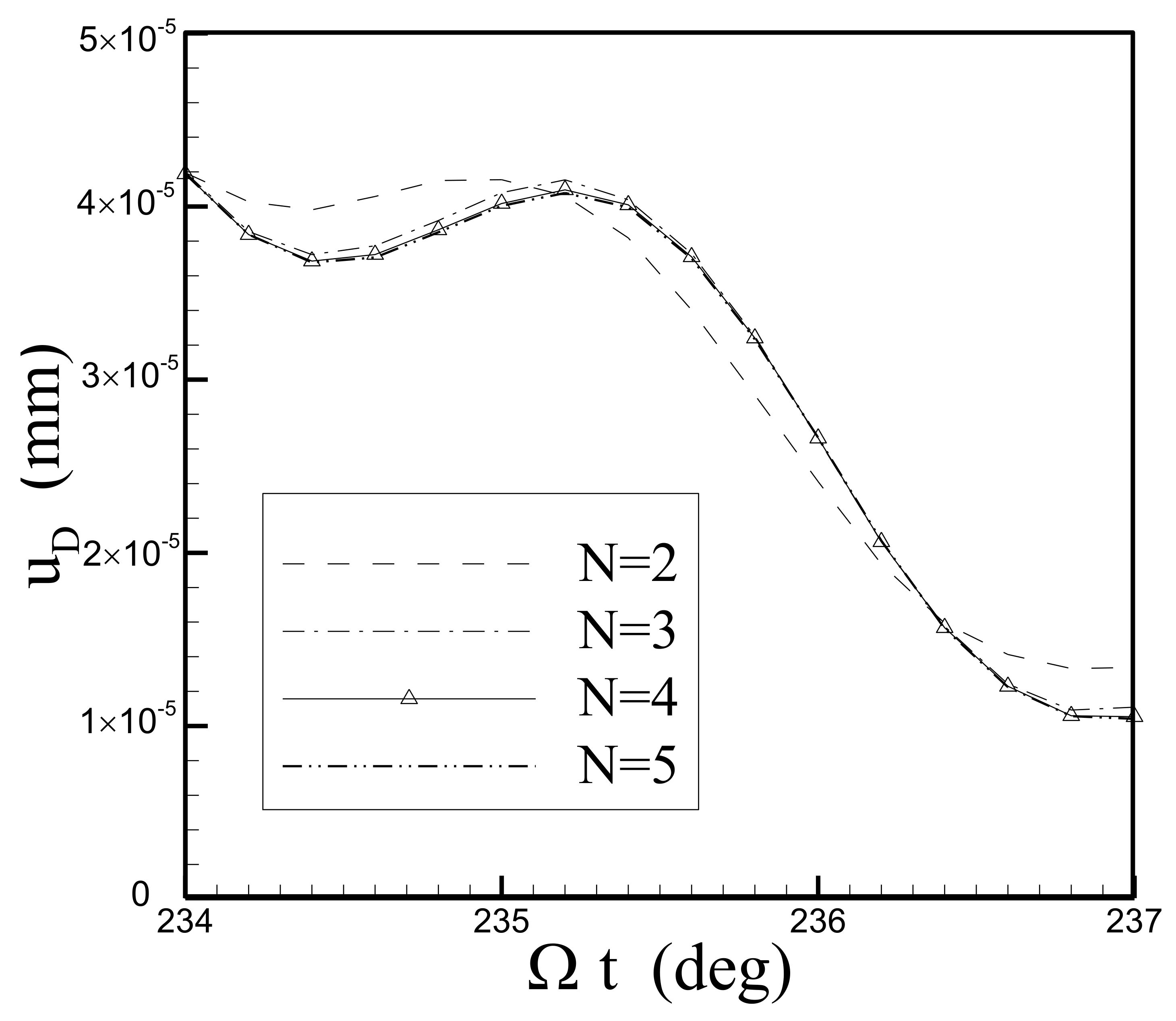
Zero initial conditions are used in this study. To verify the convergence of the assumed mode method, four numbers of modes are employed. The cycloid displacement motion used for the RDFD motion and the cam speed of 320 $\mathrm{rad}/\mathrm{s}$ are considered. The time responses of the follower output node in the lateral and axial directions are denoted as $v_D$ and $u_D$, respectively, as shown in Figure 4 and Figure 5. The curves N = 2 and N = 3 have obvious errors, and N = 4 and N = 5 nearly overlap. Because the results of the study almost converge to N = 4, N = 4 is used for the following studies.

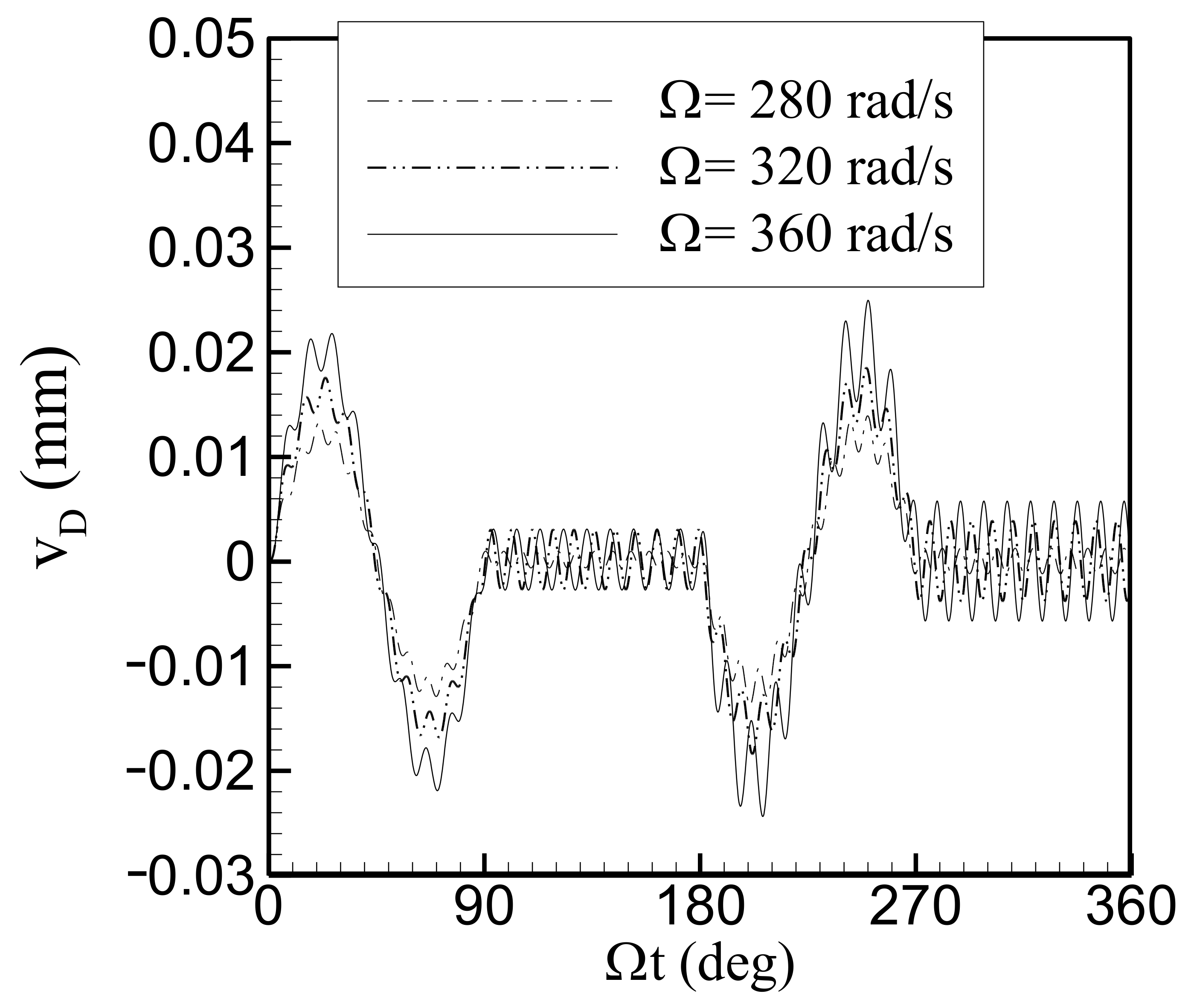
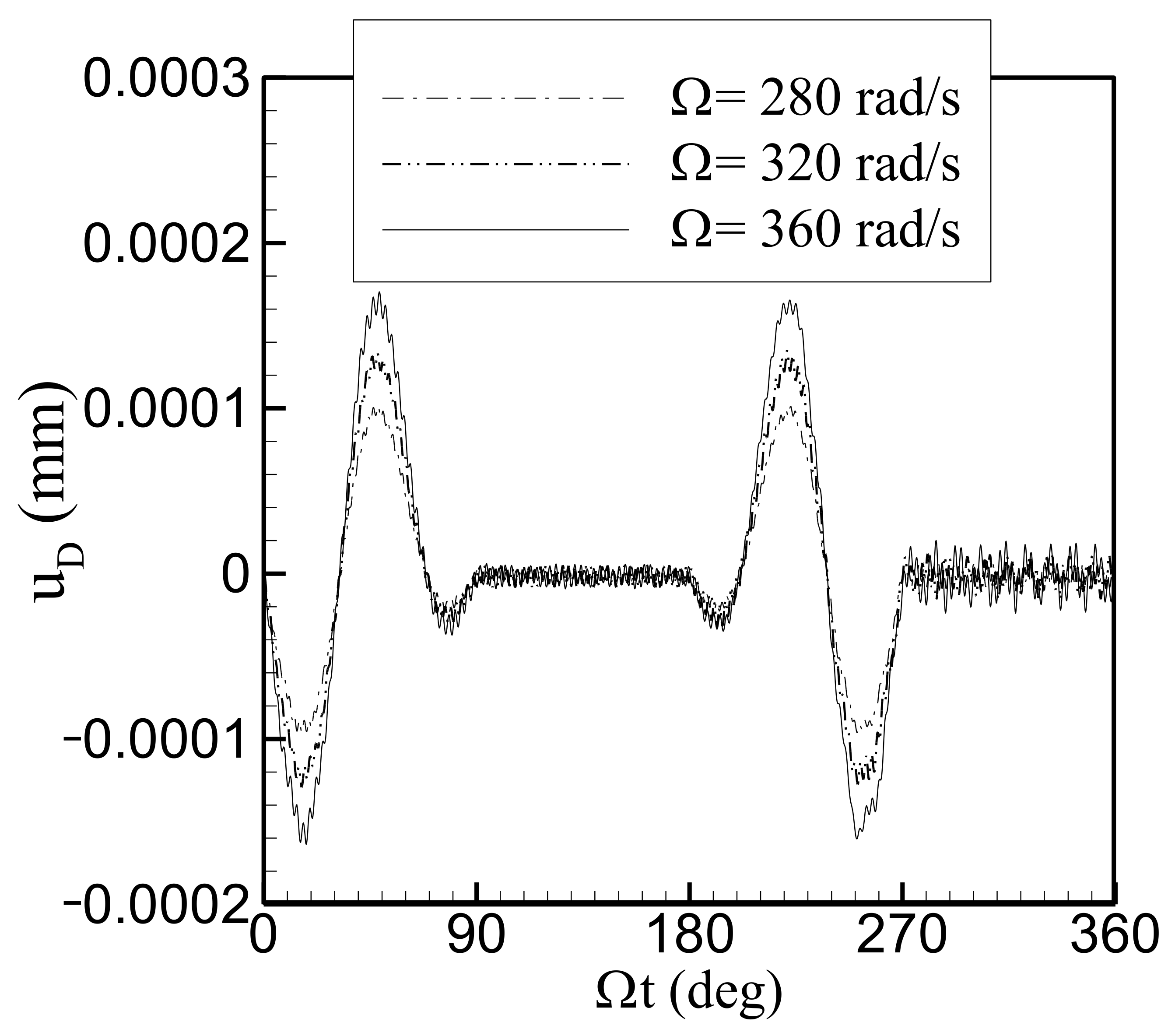
The vibration of the follower using the cycloid displacement motion for the RDFD motion at three cam speeds, specifically 280, 320, and 360 rad/s, is studied. The time responses of the follower output node in the lateral and axial directions are shown in Figure 6 and Figure 7. The time history diagram indicates that the follower contains two parts: one is the response of a large amplitude and a low frequency only in the ascending and descending cycles, and the other is the response of a small amplitude and a high frequency appearing in the whole cycle of the RDFD motion. The larger cam speed induces the larger vibration response in lateral and axial directions, simultaneously. Especially the vibration amplitude is more obvious in the ascending and descending cycles of the RDFD motion.

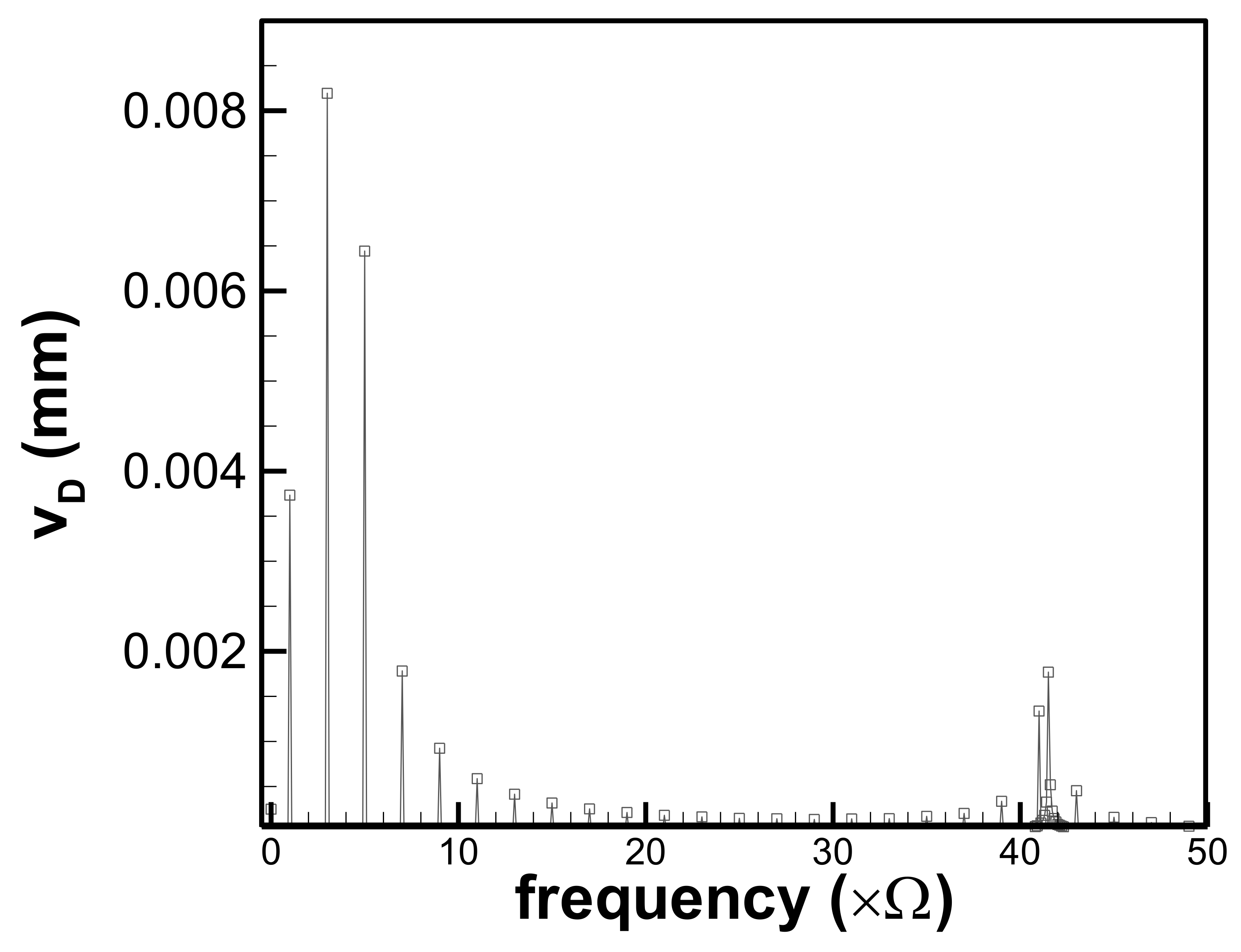
Figure 8 and Figure 9 establish the fast Fourier transform (FFT) spectrum of the follower output node under the cycloid displacement motion with $\mathsf{\Omega }=320$rad/s, which determines the cause of the high-frequency oscillation phenomenon. There are some spectral peaks at some lower frequencies that are multiples of the cam rotation speed. This may be due to the nonlinear effects. Additionally, some peaks occur at higher frequencies, near 41.5 $\mathsf{\Omega }$. To gain an insight into the vibration spectrum of the follower output node, the values of the main spectral peaks for the lateral and axial vibrations are presented, as can be found in

Table 2. The peak amplitude of the lateral vibration spectrum of the follower output node $D$ for the three RDFD motions where $\mathsf{\Omega }=$ 320 $\hspace{0.33em}\mathrm{rad}/\mathrm{s}$.

The Peak Frequency	The Three RDFD * Motions (Peak Amplitude Unit: mm)
	CD 1	MSA 2	MTA 3
$1 \mathsf{\Omega }$	3.733 × 10−3	3.704 × 10−3	3.719 × 10−3
$3 \mathsf{\Omega }$	8.194 × 10−3	7.553 × 10−3	7.905 × 10−3
$5 \mathsf{\Omega }$	6.442 × 10−3	4.596 × 10−3	5.728 × 10−3
$7 \mathsf{\Omega }$	1.782 × 10−3	4.589 × 10−4	1.300 × 10−3
$41.5 \mathsf{\Omega }$	1.769 × 10−3	2.749 × 10−3	2.205 × 10−3

* rise-dwell-fall-dwell motion, ¹ cycloid displacement motion, ² modified sinusoidal acceleration motion, ³ modified trapezoidal acceleration motion.

and

Table 3. The peak amplitudes of the axial vibration spectrum of the follower output node $D$ for the three RDFD motions where $\mathsf{\Omega }=$ 320 $\hspace{0.33em}\mathrm{rad}/\mathrm{s}$.

The Peak Frequency	The Three RDFD Motions (Peak Amplitude Unit: mm)
	CD 1	MSA 2	MTA 3
$1 \mathsf{\Omega }$	1.328 × 10−5	1.321 × 10−5	1.322 × 10−5
$2 \mathsf{\Omega }$	1.505 × 10−5	1.592 × 10−5	1.543 × 10−5
$3 \mathsf{\Omega }$	2.829 × 10−5	2.612 × 10−5	2.724 × 10−5
$4 \mathsf{\Omega }$	3.882 × 10−5	3.906 × 10−5	3.854 × 10−5
$5 \mathsf{\Omega }$	2.170 × 10−5	1.541 × 10−5	1.916 × 10−5
$6\mathsf{\Omega }$	4.413 × 10−5	3.813 × 10−5	4.020 × 10−5

^1,2,3 The same abbreviations as those in Table 2.

, respectively. Three RDFD motions with different cam profiles in the ascending and descending cycles are investigated. They include the motions of cycloid displacement (CD), modified sinusoidal acceleration (MSA), and modified trapezoidal acceleration (MTA). Table 2 and Table 3 show the peak amplitudes of the lateral and axial vibration spectra of the follower output node $D$ for the three RDFD motions with $\mathsf{\Omega }=320$rad/s, respectively. For the lateral vibration, the peaks locate mainly at the frequencies of odd multiples of cam speed $\mathsf{\Omega }$. The highest peak locates at the frequency of 3 $\mathsf{\Omega }$ for all the three RDFD motions. A small amplitude peak locates at the high frequency of 41.5 $\mathsf{\Omega }$ (13,280 rad/s). The natural frequencies of the simply supported follower are calculated, and the first three are 13,331, 53,324, and 119,978 rad/s. High-frequency components may coincide with the follower’s first natural frequency, creating a resonance condition. Although the follower rod vibrates significantly only in the ascending and descending sections, it still maintains a high-frequency vibration close to the fundamental natural frequency in the dwell section. Additionally, from the time history in Figure 6, it is also seen that the follower still vibrates with about the fundamental natural frequency during the dwell section. This means that the vibrations in the dwell part are excited mainly thanks to the fundamental frequency.

In addition, the peak amplitude depends on the cam profile. For the study case in Table 2, the peak amplitudes at frequencies $1 \mathsf{\Omega }$, $3 \mathsf{\Omega }$, $5 \mathsf{\Omega }$, and $7 \mathsf{\Omega }$ are smaller when using the modified sinusoidal acceleration motion than when using the other motions. The dominated peak is at the frequency of $3 \mathsf{\Omega }$ for the three kinds of motion. The peak amplitude around the fundamental natural frequency using the cycloid displacement motion is 1.769 × 10⁻³ mm and is smaller than those using the other motions. It is shown that different ascending and descending motions will cause different vibrational results. To reduce the lateral vibration of the follower, the selection of the cam profile from among the three motions studied is a very important factor. If low-vibration amplitudes at low frequencies ($1 \mathsf{\Omega }$, $3 \mathsf{\Omega }$, $5 \mathsf{\Omega }$, and $7 \mathsf{\Omega }$) are the primary concern, the modified sinusoidal acceleration motion is recommended. However, the corresponding vibration response of a high frequency is the most severe. If vibrations during the dwell interval are of primary concern, it is recommended to use the cycloid displacement motion to form the RDFD motion. However, it results in the maximum low-frequency-vibration response. When the modified trapezoidal acceleration motion is applied, all low- and high-frequency spectral peaks are between those using the other two motions.

For axial vibration, the main peaks listed in Table 3 are at integer multiples of the cam speed, but they are a small order of magnitude less than 10⁻⁴ mm. The largest peak occurs at the frequency of $6 \mathsf{\Omega }$ when the cycloid displacement motion is considered, and the magnitude is 4.413 × 10⁻⁵ mm. Therefore, in the following study, the table used to list the peak amplitudes of the axial vibration spectrum is ignored. It is also seen from Figure 9 that the peak amplitude of the axial displacement near the fundamental frequency is less than 10⁻⁵ mm. The first natural mode of the vibration of the follower is dominated by the transverse mode, so the excited axial displacement near the fundamental frequency is extremely small and can be ignored.

For the following parametric studies, consider a cam profile using cycloid displacement motion.

Table 4. The peak amplitude of the lateral vibration spectrum of the follower output node $D$ at three rotation speeds.

The Peak Frequency	Three Cam Rotation Speeds (rad/s) (Peak Amplitude Unit: mm)
	$\mathsf{\Omega }={280}^{ }$	$\mathsf{\Omega }=320{ }^{ }$	$\mathsf{\Omega }=360{ }^{ }$
$1 \mathsf{\Omega }$	2.839 × 10−3	3.733 × 10−3	4.746 × 10−3
$3 \mathsf{\Omega }$	6.262 × 10−3	8.194 × 10−3	1.039 × 10−2
$5 \mathsf{\Omega }$	4.914 × 10−3	6.442 × 10−3	8.189 × 10−3
$7 \mathsf{\Omega }$	1.354 × 10−3	1.782 × 10−3	2.274 × 10−3
$37.0 \mathsf{\Omega }$	-	-	1.175 × 10−2
$41.5 \mathsf{\Omega }$	-	1.769 × 10−3	-
$47.0 \mathsf{\Omega }$	1.060 × 10−3	-	-

-: the response peak is very small.

presents the spectral peak amplitudes for the three cam speeds of 280, 320, and 360 rad/s. The main peaks are at the frequencies of $1 \mathsf{\Omega }$, $3 \mathsf{\Omega }$, $5 \mathsf{\Omega }$, and $7 \mathsf{\Omega }$ and a high frequency around the fundamental frequency. The peak amplitude at the frequency of $3 \mathsf{\Omega }$ is 1.039 × 10⁻² mm at Ω = 360 rad/s, and it is larger than that at the other two cam speeds. Vibration amplitude is significantly affected by cam speed. They are larger in magnitude when higher cam rotation speeds are applied. For cam speeds of 280, 320, and 360 rad/s, the corresponding high frequencies are $47.0 \mathsf{\Omega }$ (13,160 rad/s), $41.5 \mathsf{\Omega }$ (13,280 rad/s), and $37.0 \mathsf{\Omega }$ (13,320 rad/s). They are all near the fundamental frequency 13,331 rad/s. It is found that the peak amplitude at the high frequency is 1.175 × 10⁻² mm at Ω = 360 rad/s, and it is larger than that at the other two cam speeds and even that at the frequency of $3 \mathsf{\Omega }$. When the cam rotation speed is high, the peak caused by the fundamental natural frequency is very large. This may be due to the large centrifugal effect when a high cam speed is applied. Therefore, the deformation of the follower at a high cam rotation speed during the dwell interval cannot be ignored.

The effects of parameters such as the follower length, the follower cross-sectional radius, the total follower rise, the cam base circle radius, and the torsion spring stiffness value on vibration behavior are also investigated.

Table 5. The peak amplitude of the lateral vibration spectrum of the follower output node $D$ where Ω = 320 rad/s and with three follower rod lengths.

The Peak Frequency	Three Follower Rod Lengths (mm) (Peak Amplitude Unit: mm)
	$\mathit{l}=88{ }^{ }$	$\mathit{l}=98{ }^{ }$	$\mathit{l}=108{ }^{ }$
$1 \mathsf{\Omega }$	2.169 × 10−3	3.733 × 10−3	6.104 × 10−3
$3 \mathsf{\Omega }$	4.788 × 10−3	8.194 × 10−3	1.336 × 10−2
$5 \mathsf{\Omega }$	3.753 × 10−3	6.442 × 10−3	1.055 × 10−2
$7 \mathsf{\Omega }$	1.031 × 10−3	1.782 × 10−3	2.938 × 10−3
$34.2 \mathsf{\Omega }$	-	-	3.127 × 10−3
$41.5 \mathsf{\Omega }$	-	1.769 × 10−3	-
$51.0 \mathsf{\Omega }$	7.583 × 10−4	-	-

-: the response peak is very small.

shows the peak amplitudes of the lateral vibration spectrum of the follower output node under the cycloid displacement motion where Ω = 320 rad/s using three rod lengths, specifically 88, 98, and 108 mm. The peaks of $l=$108 mm are much higher than those of the other two cases. The main peak amplitude occurring at the frequency of $3 \mathsf{\Omega }$ is $1.336\times {10}^{-2}$ mm for the case of $l=$108 mm. It is found that the rod length significantly influences the main peak magnitude. This can be explained by the fact that a longer follower makes the rod less stiff, resulting in a greater response. For the 88, 98, and 108 mm rod lengths, the peak frequencies at a high frequency are $51.0 \mathsf{\Omega }$, $41.5 \mathsf{\Omega }$, and $34.2 \mathsf{\Omega }$, respectively, calculated as 16,320, 13,280, and 10,944 rad/s. The fundamental natural frequencies of follower vibration are also calculated as 16,533, 13,331, and 10,976 rad/s for the three rod lengths of 88, 98, and 108 mm, respectively. The high frequency is close to the fundamental natural frequency. For low vibration, a short follower is recommended.

The response spectra of the three circular cross-sectional radii 4, 5, and 6 mm of the follower are shown in

Table 6. The peak amplitude of the lateral vibration spectrum of the follower output node $D$ where Ω = 320 rad/s and with three follower rod radii.

The Peak Frequency	Three Follower Rod Radii (mm) (Peak Amplitude Unit: mm)
	${\mathit{r}}_{\mathit{f}}=4{ }^{ }$	${\mathit{r}}_{\mathit{f}}=5{ }^{ }$	${\mathit{r}}_{\mathit{f}}=6{ }^{ }$
$1 \mathsf{\Omega }$	5.753 × 10−3	3.733 × 10−3	2.610 × 10−3
$3 \mathsf{\Omega }$	1.281 × 10−2	8.194 × 10−3	5.686 × 10−3
$5 \mathsf{\Omega }$	1.015 × 10−2	6.442 × 10−3	4.456 × 10−3
$7 \mathsf{\Omega }$	2.837 × 10−3	1.782 × 10−3	1.227 × 10−3
$33.3 \mathsf{\Omega }$	8.055 × 10−3	-	-
$41.5 \mathsf{\Omega }$	-	1.769 × 10−3	-
$49.8 \mathsf{\Omega }$	-	-	6.525 × 10−4

-: the response peak is very small.

. The peaks of $r_f=4$ mm are higher than those of the other two cases. The dominated peak amplitude occurring at the frequency of $3 \mathsf{\Omega }$ is 1.281 × 10⁻² mm for the case of $r_f=4$ mm. For the 4, 5, and 6 mm rod radii, the peak frequencies at a high frequency are $33.3 \mathsf{\Omega }$, $41.5 \mathsf{\Omega }$, and $49.8 \mathsf{\Omega }$, respectively, calculated as 10,656, 13,280, and 15,936 rad/s. The corresponding fundamental natural frequencies of follower vibration are also calculated as 10,665, 13,331, and 15,998 rad/s. It is seen that the high frequency is close to the fundamental natural frequency. The radius of the circular cross section of the follower significantly influences the main peak magnitude. The smaller the follower’s cross-sectional radius, the greater the vibration response. This is interpreted as follows: the smaller the follower’s cross-sectional radius, the lower the follower’s stiffness. It recommended that the radius of the circular section of the follower be large to reduce the vibration of the follower.

The three total ascents ${\phi }_T$ of $\frac{\pi }{24}$, $\frac{\pi }{18}$, and $\frac{\pi }{12}$ rad are also investigated. The results seen from

Table 7. The peak amplitude of the lateral vibration spectrum of the follower output node $D$ where Ω = 320 rad/s and with three total rises.

The Peak Frequency	Three Total Rises (rad) (Peak Amplitude Unit: mm)
	${\mathit{\phi }}_{\mathit{T}}=\frac{\mathit{\pi }}{24}$	${\mathit{\phi }}_{\mathit{T}}=\frac{\mathit{\pi }}{18}$	${\mathit{\phi }}_{\mathit{T}}=\frac{\mathit{\pi }}{12}$
$1 \mathsf{\Omega }$	2.800 × 10−3	3.733 × 10−3	5.601 × 10−3
$3 \mathsf{\Omega }$	6.146 × 10−3	8.194 × 10−3	1.229 × 10−2
$5 \mathsf{\Omega }$	4.833 × 10−3	6.442 × 10−3	9.663 × 10−3
$7 \mathsf{\Omega }$	1.337 × 10−3	1.782 × 10−3	2.670 × 10−3
$41.5 \mathsf{\Omega }$	1.321 × 10−3	1.769 × 10−3	2.701 × 10−3

show that the peaks of ${\phi }_T=\frac{\pi }{12}$ rad are higher than those of the other two cases. The dominated peak amplitude occurring at the frequency of $3 \mathsf{\Omega }$ is 1.229 × 10⁻² mm for the case of ${\phi }_T=\frac{\pi }{12}$ rad. A larger total follower rise results in a larger follower vibration response. The magnitude of the peak is also found to be almost proportional to the total rise, e.g., $\frac{\pi }{24}:\frac{\pi }{18}:\frac{\pi }{12} \cong$$6.146\times {10}^{-3}:8.194\times {10}^{-3}:1.229\times$$:{10}^{-2}$ for the frequency of $3 \mathsf{\Omega }$.

Three cam base circle radii are investigated. In

Table 8. The peak amplitude of the lateral vibration spectrum of the follower output node $D$ case where Ω = 320 rad/s and with three cam base circle radii.

The Peak Frequency	Three Cam Base Circle Radii (mm) (Peak Amplitude Unit: mm)
	${\mathit{r}}_{\mathit{b}}={60}^{ }$	${\mathit{r}}_{\mathit{b}}=66{ }^{ }$	${\mathit{r}}_{\mathit{b}}=72{ }^{ }$
$1 \mathsf{\Omega }$	3.733 × 10−3	3.733 × 10−3	3.733 × 10−3
$3 \mathsf{\Omega }$	8.202 × 10−3	8.194 × 10−3	8.192 × 10−3
$5 \mathsf{\Omega }$	6.448 × 10−3	6.442 × 10−3	6.441 × 10−3
$7 \mathsf{\Omega }$	1.783 × 10−3	1.782 × 10−3	1.782 × 10−3
$41.5 \mathsf{\Omega }$	1.823 × 10−3	1.769 × 10−3	1.756 × 10−3

, the peaks of $r_b=60$ mm are a little higher than those of the other two cases. However, it can be seen that the peak amplitude varies little with the cam base circle radius. The dominated peak amplitude occurring at the frequency of $3 \mathsf{\Omega }$ is 8.202 × 10⁻³ mm for the case of $r_b=60$ mm. The effect of the cam base circle radius on follower vibration amplitude appears to be negligible. The high frequency of 41.5 $\mathsf{\Omega }$ (13,280 rad/s), the same as that in Table 2, nears the fundamental natural frequency of 13,331 rad/s.

Three values are used to discuss the effect of torsion spring stiffness. It can be seen from

Table 9. The peak amplitude of the lateral vibration spectrum of the follower output node $D$ where Ω = 320 rad/s and with three torsion spring stiffness coefficients.

The Peak Frequency	Three Torsion Spring Coefficients (kg·mm2/s2) (Peak Amplitude Unit: mm)
	${\mathit{k}}_{\mathit{s}}=0{ }^{ }$	${\mathit{k}}_{\mathit{s}}=1.44\times {10}^5$	${\mathit{k}}_{\mathit{s}}=1.44\times {10}^6$
$1 \mathsf{\Omega }$	3.818 × 10−3	3.733 × 10−3	3.971 × 10−3
$3 \mathsf{\Omega }$	8.215 × 10−3	8.194 × 10−3	8.010 × 10−3
$5 \mathsf{\Omega }$	6.448 × 10−3	6.442 × 10−3	6.390 × 10−3
$7 \mathsf{\Omega }$	1.782 × 10−3	1.782 × 10−3	1.774 × 10−3
$41.5 \mathsf{\Omega }$	1.788 × 10−3	1.769 × 10−3	1.617 × 10−3

that the peaks of k_s = 0 kg·mm²/s² are higher than those of the other two cases. The larger the stiffness coefficient of the torsion spring, the smaller the peak amplitude, though the change is small. The dominated peak amplitude occurring at the frequency of $3 \mathsf{\Omega }$ is 8.215 × 10⁻³ mm for the case of k_s = 0 kg·mm²/s². The high frequency of 41.5 $\mathsf{\Omega }$ (13,280 rad/s), the same as that in Table 2, nears the fundamental natural frequency of 13,331 rad/s.

5. Conclusions

Thanks to the time-dependent boundary effect caused by the axial and lateral displacements of the follower, two geometric constraints are successfully formulated and multiplied by Lagrangian multipliers to add to the variational principle, to establish the vibration equation of the motion of the follower of the oscillating follower cam system. The new findings of the present study are as follows:

(1)

The coupled axial and lateral vibration of the continuous flexible follower has been studied for the first time. The major spectral peaks for the lateral follower response located at the low frequencies of $1 \mathsf{\Omega }$, $3 \mathsf{\Omega }$, $5 \mathsf{\Omega }$, and $7 \mathsf{\Omega }$ and the high frequency near the fundamental frequency. The dominated peak located at the frequency $3 \mathsf{\Omega }$, except that the cam rotated at a high speed. The axial follower response was very small compared with the lateral response.

(2)

The follower vibrations under three motion conditions, cycloid displacement motion, modified sinusoidal acceleration motion, and modified trapezoidal acceleration motion, were studied. Important new results were found: while the curves for the three kinds of motion nearly coincided, the vibrational outcomes of the follower considerably varied. The magnitude of the main lateral peaks at low frequencies was minimal by using the modified sinusoidal acceleration motion. When using the cycloid displacement motion, the lateral peak amplitude around the fundamental natural frequency of the follower was minimal.

Though the convergence of the assumed mode method has been considered and discussed, it is recommended that future work needs to verify and improve the results’ accuracy by setting up experiments and adding some other numerical methods.