Article

A Super-Convergent Stochastic Method Based on the Sobol Sequence for Multidimensional Sensitivity Analysis in Environmental Protection

1
Institute of Information and Communication Technologies, Bulgarian Academy of Sciences, Acad. G. Bonchev Str. Bl. 25A, 1113 Sofia, Bulgaria
2
Institute of Mathematics and Informatics, Bulgarian Academy of Sciences, Acad. G. Bonchev Str. Bl. 8, 1113 Sofia, Bulgaria
3
Department of Applied Mathematics and Statistics, University of Ruse, 8 Studentska Str., 7004 Ruse, Bulgaria
*
Author to whom correspondence should be addressed.
Axioms 2023, 12(2), 146; https://doi.org/10.3390/axioms12020146
Submission received: 20 December 2022 / Revised: 26 January 2023 / Accepted: 27 January 2023 / Published: 31 January 2023
(This article belongs to the Special Issue Advances in Stochastic Modelling)

Abstract

:
Environmental security is among the top priorities worldwide, and there are many difficulties in this area. The reason for this is a painful subject for society and healthcare systems. Multidimensional sensitivity analysis is fundamental in the process of validating the accuracy and reliability of large-scale computational models of air pollution. In this paper, we present an improved version of the well-known Sobol sequence, which shows a significant improvement over the best available existing sequences in the measurement of the sensitivity indices of the digital ecosystem under consideration. We performed a complicated comparison with the best available low-discrepancy sequences for multidimensional sensitivity analysis to study the model’s output with respect to variations in the input emissions of anthropogenic pollutants and to evaluate the rates of several chemical reactions. Our results, which are presented in this paper through a sensitivity analysis, will play an extremely important multi-sided role.

1. Introduction

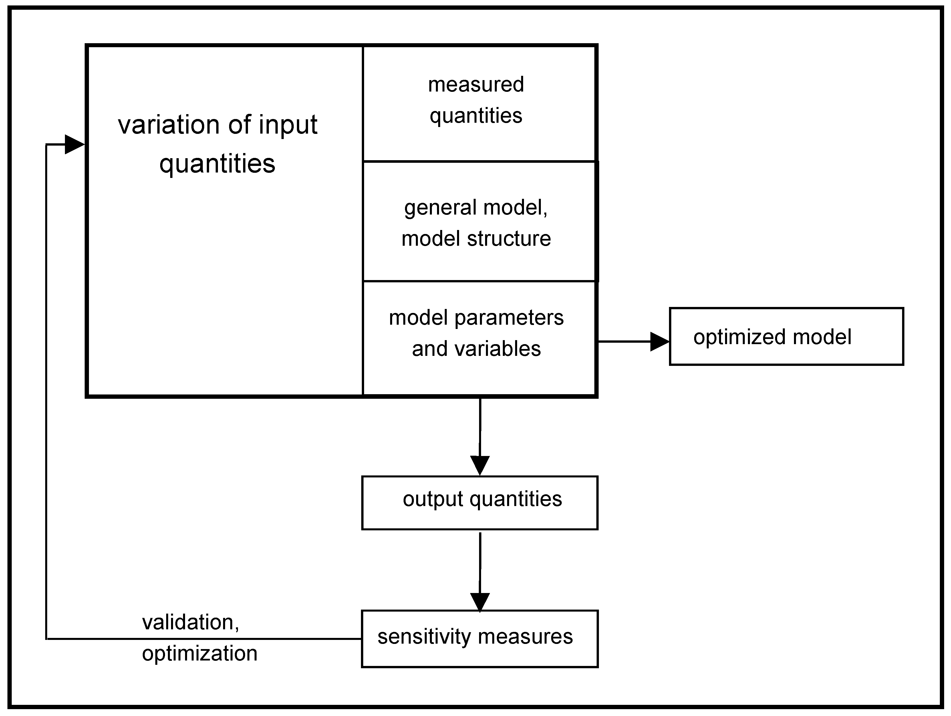
The purpose of our work is in the field of environmental security [1,2], since this is one of the key areas worldwide. By definition, a sensitivity analysis (SA) is an investigation of how much the uncertainty in the input data of a model is apportioned in the accuracy of the output results [3,4,5,6,7]; see Figure 1. Multidimensional SA [8,9,10,11,12] is a very challenging task when modeling, but it is often the key tool for studying a complex phenomenon [13,14,15,16,17].
The main problem in SA is the evaluation of the total sensitivity indices (SIs) [18,19,20,21]. The mathematical formulation for estimating the SIs is represented by a set of multidimensional integrals (MIs) [22,23,24,25]. The Monte Carlo (MC) and quasi-Monte Carlo (QMC) methods are the best tools for solving the MIs [22,26,27,28,29,30,31]. For a more clear explanation of the objectives in this paper, one should check [32,33,34].
The input data for SA were obtained with a large-scale model of the long-range transport of pollutants in the air—the Unified Danish Eulerian Model (UNI-DEM) [35,36,37,38,39]. UNI-DEM is also a basic tool and important tool for the creation of a digital twin, namely, Digital Air (see [40]).
By definition, the model can be introduced with a model function [41]:
u = f ( x ) , x = ( x 1 , x 2 , , x d ) U d [ 0 , 1 ] d .
The concept of the Sobol approach consists of the following representation of f ( x ) and a constant f 0 [41]:
f ( x ) = f 0 + ν = 1 d l 1 < < l ν f l 1 l ν ( x l 1 , x l 2 , , x l ν ) .
The above description is noted as the ANOVA representation of f ( x ) if [41]:
0 1 f l 1 l ν ( x l 1 , x l 2 , , x l ν ) d x l k = 0 , 1 k ν , ν = 1 , , d .
The quantities
D = U d f 2 ( x ) d x f 0 2 , D l 1 l ν = f l 1 l ν 2 d x l 1 d x l ν
are called total and partial variances [41]. The same is true for the total variance:
D = ν = 1 d l 1 < < l ν D l 1 l ν .
The Sobol global SIs [6,41] are determined by:
S l 1 l ν = D l 1 l ν D , ν { 1 , , d } .
Then, the total sensitivity index (TSI) of the input parameter x i , i { 1 , , d } is determined by [42]:
T S I ( x i ) = S i + l 1 i S i l 1 + l 1 , l 2 i , l 1 < l 2 S i l 1 l 2 + + S i l 1 l d 1 ,
where S i l 1 l j 1 is the jth-order SI for x i ( 2 j d ) .
According to the definition in [43], when j = 1 , the quantity S i is called the main effect of x i ; if j = 2 , S i j are called two-way interactions (second-order SIs); if j = 3 , S i j k are called three-way interactions (third-order SIs), and so on. In this study, we are interested in the main effects and the two-way interactions.
The TSI of the output variance for an input parameter x i , i { 1 , , d } is represented as: S T i = S i + j i S i j + j i , k i , j < k S i j k + ; see [18]. With this, we show that multidimensional SA using Sobol’s approach is turned into a problem of evaluating MIs [44].
In this paper, we aim to suggest implementations for the fast and accurate evaluation of the sensitivity indices. As mentioned earlier, the problem of SA is transformed into a multidimensional integration task that is approached by using novel quasi-Monte Carlo methods, which are compared with the best available algorithms in an application to large-scale modeling of atmospheric pollution. The methods are described in the next section, followed by a thorough analysis of the computational results.

2. Methods and Algorithms

Consider the following multidimensional problem:
S ( f ) : = I = U s f ( x ) d x ,
where x ( x 1 , , x s ) U s R s and f C ( U s ) .
In the simplest possible MC approach, “Crude”, we introduce the random variable θ = f ( ξ ) , for which
E θ = Ω f ( x ) p ( x ) d x ,
and the random points ξ 1 , ξ 2 , , ξ N are independent realizations of the random point ξ with a probability density function p ( x ) and θ 1 = f ( ξ 1 ) , , θ N = f ( ξ N ) . The Crude MC approach for the integral I is defined as [22]:
θ ¯ N = 1 N i = 1 N θ i .
Let x i = ( x i ( 1 ) , x i ( 2 ) , , x i ( s ) ) for i = 1 , 2 , and let n = a 3 ( n ) , a 2 ( n ) , a 1 ( n ) be the representation of n in base b .
Then, the discrepancy (star discrepancy) of the set is defined [22,24]:
D N * = D N * ( x 1 , , x N ) = sup Ω E s # { x n Ω } N V ( Ω ) ,
where E s = [ 0 , 1 ) s .
For the one-dimensional quasi-random number sequence, we introduce the radical inverse sequence [22,23]:
n = i = 0 a i + 1 ( n ) b i , ϕ b ( n ) = i = 0 a i + 1 ( n ) b ( i + 1 ) .
The van der Corput sequence [45] is obtained when b = 2 . Now, the multidimensional quasi-random number sequence is defined as: X n = ( ϕ b 1 ( n ) , ϕ b 2 ( n ) , , ϕ b s ( n ) ) , where the bases b i are all relatively prime: ( b 1 , b 2 , , b s ) ( 2 , 3 , 5 , , p s ) , where p i denotes the ith prime.
Now, the Halton sequence [46,47] is defined as:
s n ( k ) = i = 0 σ i + 1 ( k ) a i + 1 ( k ) ( n ) b k ( i + 1 ) ,
where ( b 1 , b 2 , , b s ) ( 2 , 3 , 5 , , p s ) , p i designates the i-th prime, and σ i ( k ) , i 1 denotes the set of permutations on ( 0 , 1 , 2 , , p k 1 ) .
The standard M-dimensional Hammersley sequence [48], which is based on N samples, is simply composed of a first component of successive fractions 0 / N , 1 / N , , N / N paired with M 1 one-dimensional van der Corput sequences by using the first M 1 primes as bases. More precisely, if p 1 , p 2 , , p s 1 are the first s 1 prime numbers, then the Hammersley sequence { t 0 , t 1 , , t N 1 } with N points in s dimensions is given by
t i = i / n , ϕ p 1 ( i ) , ϕ p 2 ( i ) , , ϕ p s 1 ( i ) , i = 0 , 1 , , N 1 .
The Faure sequence [49,50,51] is given by:
x n ( k ) = i = 0 a i + 1 ( n ) q ( i + 1 ) , k = 1 j = 0 c j + 1 q ( j + 1 ) , k 2 , where j 1 ,
c j = i j ( k 1 ) i j i ! ( i j ) ! j ! a i ( n ) ( mod q ) , q is   a   prime ( q s 2 ) .
The Sobol sequence [52,53,54] is defined by:
x k σ ¯ i ( k ) , k = 0 , 1 , 2 ,
where σ ¯ i ( k ) , i 1 are the set of permutations on every 2 k , k = 0 , 1 , 2 , subsequent points of the van der Corput sequence, defined by n = i = 0 a i + 1 ( n ) b i , ϕ b ( n ) = i = 0 a i + 1 ( n ) b ( i + 1 ) when b = 2 .
In binary, for the Sobol sequence, we have that: x n ( k ) = i 0 a i + 1 ( n ) v i , where v i , i = 1 , , s is the set of directional numbers [55].
For the QMC algorithms, based on the Halton, Faure and Sobol sequences, it is known that the corresponding discrepancy is:
D N * = O log s N N .
According to several important works [56,57,58,59], the convergence rate for the scrambling algorithms essentially improves the convergence rate for the unscrambled nets [56,57,58,59], which is N 1 ( log N ) s 1 . The scrambling itself is based on the randomization of a single digit at each iteration. Let
x ( i ) = ( x i , 1 , x i , 2 , , x i , s ) , i = 1 , , n
be quasi-random numbers in [ 0 , 1 ) s , and let
z ( i ) = ( z i , 1 , z i , 2 , , z i , s )
be the corresponding scrambled version of the point x ( i ) . Let every x i , j be rewritten in base b as
x i , j = ( 0 . x i 1 , j x i 2 , j x i K , j ) b ,
with K being the number of digits for scrambling. For the scrambled Halton sequence HaltonScr, we apply a permutation of the radical inverse coefficients, which is obtained by applying a reverse-radix operation to each of the possible coefficient values [60]. For the scrambled Sobol sequence SobolScr, we use a random linear scramble blended with a random digital shift [61].
Now, we will introduce a super-convergent modified Sobol sequence SobolBurkardt based on the INSOBL and GOSOBL routines in ACM TOMS Algorithm 647 and ACM TOMS Algorithm 659, as well as a Burkardt modification [52,53,54,55,62,63,64,65,66,67]. The original code can only compute the next element of the sequence. Our modification allows the user to specify the index of the desired element. The novelty is that this is the first time that the SobolBurkardt algorithm has been applied for a multidimensional sensitivity analysis of this important digital ecosystem.

3. Results and Discussion

In this section, the advanced stochastic algorithms described above (Crude, Sobol, Halton, SobolScr, HaltonScr, SobolBurkardt, Hammersley, and Faure) are applied to sensitivity studies with respect to emission levels (SSREL) and with respect to some chemical reaction rates (SSRCRR) of varying concentrations of UNI-DEM pollutants [68,69]. We use the following notations: EQ refers to the estimated quantity, RV refers to the reference value, RE refers to the relative error, and AE refers to the approximate evaluation.
For SSREL, we will investigate an SA of the model output (in terms of the mean monthly concentrations of several important pollutants—in our case, the pollutant is ammonia in Milan) with respect to a variation in the input emissions from anthropogenic pollutants, which consist of four components, E = ( E A , E N , E S , E C ) :
E A ammonia ( NH 3 ) ; E S sulphur   dioxide ( SO 2 ) ; E N nitrogen   oxides ( NO + NO 2 ) ; E C anthropogenic   hydrocarbons .
The output of the model is the mean monthly concentration of the following three pollutants:
s 1 —ozone ( O 3 );
s 2 —ammonia ( NH 3 );
s 3 —ammonium sulfate and ammonium nitrate ( NH 4 SO 4 + NH 4 NO 3 ).
For SSEL, the results for the REs for the AE of the f 0 , D , S i and S i tot when using Crude, Sobol, Halton, SobolScr, HaltonScr, SobolBurkardt, Hammersley, Faure are shown in Table 1, Table 2, Table 3, Table 4, Table 5 and Table 6, respectively. The quantity f 0 is represented by a four-dimensional integral, whereas the rest are represented by eight-dimensional integrals.
In the case of SSRCRR, we will investigate the ozone concentrations in Genova according to the rates of variation of these chemical reactions, which are ## 1 , 3 , 7 , 22 (time-dependent) and 27 , 28 (time-independent) in the CBM-IV scheme [36]:
[ # 1 ] NO 2 + h ν NO + O ; [ # 22 ] HO 2 + NO OH + NO 2 ; [ # 3 ] O 3 + NO NO 2 ; [ # 27 ] HO 2 + HO 2 H 2 O 2 ; [ # 7 ] NO 2 + O 3 NO 3 ; [ # 28 ] OH + CO HO 2 .
In the case of SSRCRR, the results for the REs for the AE of f 0 , D , S i , S i j and S i tot when using Crude, Sobol, Halton, SobolScr, HaltonScr, SobolBurkardt, Hammersley, and Faure are shown in Table 7, Table 8, Table 9, Table 10, Table 11 and Table 12, respectively. As in the first case study, the quantity f 0 is represented by a six-dimensional integral, whereas the rest are represented by twelve-dimensional integrals.
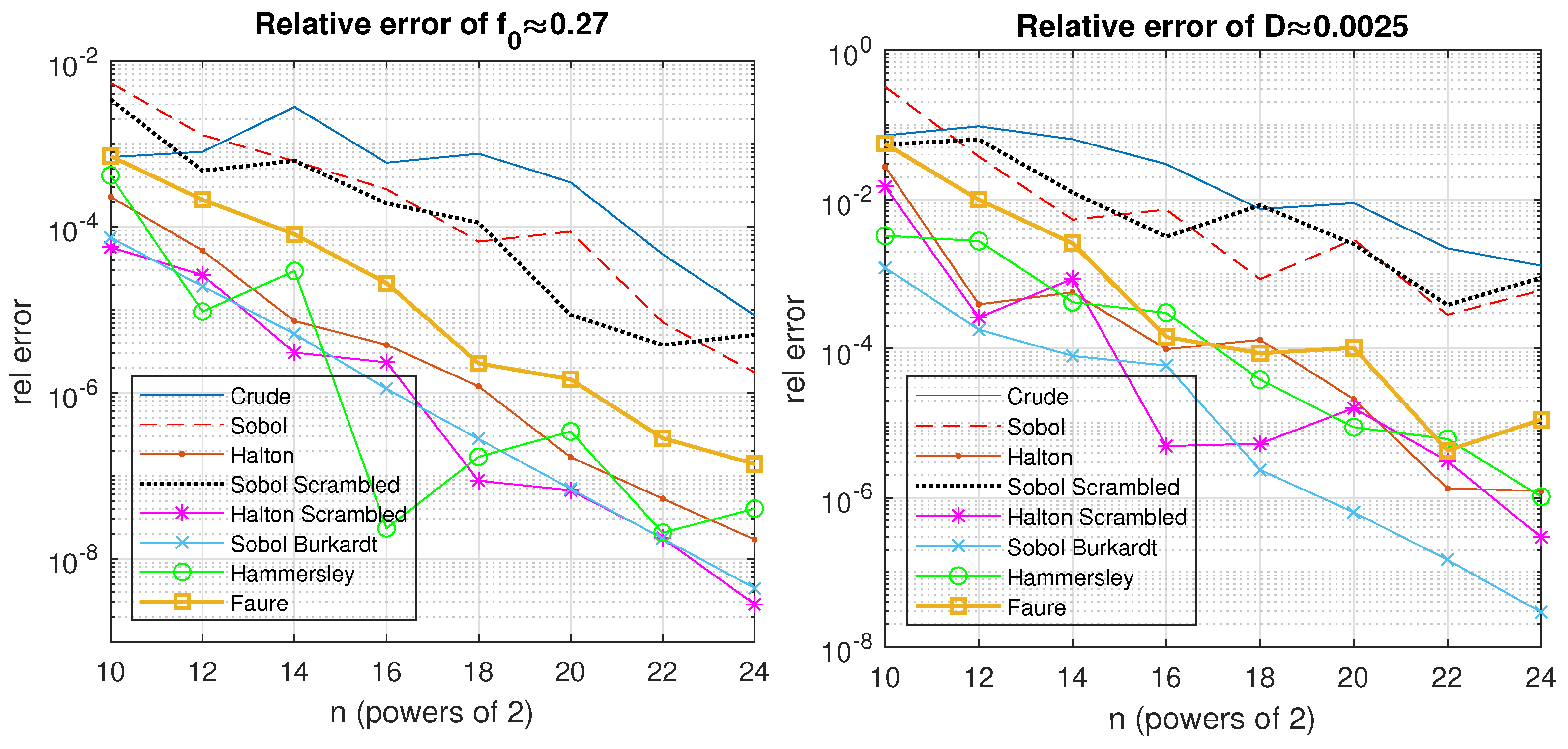
In the case of SSREL, one may observe the following. In Table 1, for the model function f 0 , the best algorithm for all numbers of samples is HaltonScr, followed by SobolBurkardt. For N = 2 24 , for the total variance D , the best algorithm is SobolBurkardt, followed by the Halton sequence—see the results in Table 2. However, for N = 2 18 and N = 2 22 , the Halton sequence produces slightly better results—see Table 2. The behavior of the algorithm can also be seen in Figure 2. The RVs for the first and total SIs are presented in Table 3. From Table 4, Table 5 and Table 6, one can conclude that for all first-order SIs and TSIs, the best algorithm is SobolBurkardt, followed by HaltonScr and the Halton sequence. It is important that the scrambling procedure improves the results of the Sobol and Halton sequences by at least one order for most of the cases—see the values for S 2 tot and S 3 tot in Table 6. In [42], it was pointed out that having the smallest possible SIs is the most important aspect of a model. In our case, these are S 4 and S 4 tot —see Table 3. For them, SobolBurkardt significantly improved upon the results of the other sequences, and one can also see that the Hammersley and Faure sequences performed better than the Crude algorithm, as expected.
The performance of the algorithms in the case of SSREL can be generalized in this way: The algorithm that we implemented, SobolBurkardt, held the smallest relative errors for all SIs; the scrambled Halton and original Halton sequences were the next, followed by the Hammersley, Faure, scrambled Sobol, and Sobol algorithms; the worst was the plain algorithm.
In the case of SSRCRR, the following observations could be made. In Table 7, for the model function f 0 , the best algorithm for all numbers of samples except N = 2 12 , N = 2 16 , and N = 2 22 was HaltonScr; for N = 2 22 , the best algorithm was SobolBurkardt, and in the other two cases, the best algorithm was the Hammersley sequence. The RVs of the first- and second-order SIs and TSIs are given in Table 9. For all numbers of samples except N = 2 16 , for the total variance D, the best algorithm was SobolBurkardt—see the results in Table 8. However, for N = 2 16 , the scrambled Halton sequence produced results that was one order better than our SobolBurkardt algorithm. The behavior of the algorithm can also be seen in Figure 3. For a low number of samples, N = 2 16 , as shown in Table 10, the Halton sequence was better than our SobolBurkardt algorithm for S 4 and S 6 , and the scrambled Halton sequence was better than our algorithm for the total SIs S 1 tot , S 2 tot , and S 4 tot . As previously mentioned, having the smallest possible SIs is the most important aspect of a model. Here, these were S 5 , S 45 , and S 5 tot —see Table 9. For them, our SobolBurkardt implementation performed better than the other algorithms. However, for larger numbers of samples, as shown in Table 11 and Table 12, one can conclude that for all first-order SIs, second-order SIs, and TSIs, the best algorithm was SobolBurkardt, followed by the HaltonScr and scrambled Sobol sequence algorithms. It is important that the scrambling procedure significantly improved the results of the Sobol and Halton sequences for some of the cases—see the values for S 4 and S 6 in Table 12. For all of the cases, the Hammersley and Faure sequences performed better than the Crude algorithm, as expected.
The performance of the algorithms in the case of SSREL can be generalized in such a way: The SobolBurkardt algorithm that we implemented held the smallest REs for all SIs; the scrambled Halton and the original Halton sequence are the next, followed by the Hammersley, Faure, scrambled Sobol, and Sobol algorithms, and the worst was the Crude algorithm.
The overall conclusion is that the implemented SobolBurkardt algorithm was the best approach among the benchmarked algorithms, and the values of the relative errors showed its supremacy over the majority of the existing methods when applied to multidimensional air pollution sensitivity analysis.

4. Conclusions

Our paper treats a very important area of environmental safety. The computational accuracy and numerical efficiency in terms of the relative error for one of the best available stochastic methods for multidimensional integration were studied for the sensitivity of the Unified Danish Eulerian model’s output to find the variations in the rate constants of chosen chemical reactions and the variations in selected input emissions of anthropogenic pollutants. We implemented an improved Sobol sequence based on a Burkardt modification, which dramatically improved upon the results produced by other low-discrepancy sequences that have been used until now to perform multidimensional sensitivity analyses of this model. In addition, for the first time, we included the Faure and Hammersley sequences in our comparison; they have never before been compared with the Sobol and Halton sequences for this particular and very important large-scale air pollution model.
When compared with the results reported in recent studies, our results show significant improvements in terms of the accuracy and lower computational costs of the suggested algorithm. Our improvements when calculating the sensitivity indices of the model will significantly help provide a more accurate evaluation of agricultural losses. The most important effect of our results will be our contribution to the estimation of harmful emissions’ effects on human health.
There are many ways in which this investigation could be extended. Some of the straightforward ones include exploring other quasi-sequences with possibly better properties, scrambling and shifting the existing sequences, and creating new ones from suitable generation vectors or generation matrices.

Author Contributions

Conceptualization, V.T.; methodology, V.T.; software, V.T. and S.G.; validation, V.T. and S.G.; formal analysis, V.T.; investigation, V.T.; resources, V.T.; data curation, V.T. and S.G.; writing—original draft preparation, V.T. and S.G.; writing—review and editing, I.D., V.T. and S.G.; visualization, V.T. and S.G.; supervision, I.D. and V.T.; project administration, I.D. and V.T.; funding acquisition, I.D. All authors have read and agreed to the published version of the manuscript.

Funding

The development of stochastic methods was supported by the Bulgarian National Science Fund under Bilateral Project KP-06-Russia/17 “New Highly Efficient Stochastic Simulation Methods and Applications”. The Sobol global approach estimation was supported by the Bulgarian National Science Fund under Project KP-06-M32/2—17.12.2019 “Advanced Stochastic and Deterministic Approaches for Large-Scale Problems of Computational Mathematics”. The multidimensional sensitivity analysis was supported by the Bulgarian National Science Fund under Project KP-06-N52/5 “Efficient methods for modeling, optimization and decision making”. The optimization of the Sobol algorithm was supported by the Bulgarian National Science Fund under Project KP-06-N62/6 “Machine learning through physics-informed neural networks”. The experimental study was supported by the National Program “Young Scientists and Postdoctoral Researchers-2”—Bulgarian Academy of Sciences.

Institutional Review Board Statement

Not applicable.

Informed Consent Statement

Not applicable.

Data Availability Statement

Not applicable.

Conflicts of Interest

The authors declare no conflict of interest.

References

  1. Havasi, Á.; Bartholy, J.; Faragó, I. Splitting method and its application in air pollution modeling. Idojárás 2001, 105, 39–58. [Google Scholar]
  2. Fidanova, S.; Zhivkov, P.; Roeva, O. InterCriteria Analysis Applied on Air Pollution Influence on Morbidity. Mathematics 2022, 10, 1195. [Google Scholar] [CrossRef]
  3. Ferretti, F.; Saltelli, A.; Tarantola, S. Trends in sensitivity analysis practice in the last decade journal. Sci. Total Environ. 2016, 568, 666–670. [Google Scholar] [CrossRef]
  4. Saltelli, A.; Chan, K.; Scott, M. Sensitivity Analysis; John Wiley & Sons Publishers: London, UK, 2000. [Google Scholar]
  5. Saltelli, A.; Tarantola, S.; Chan, K. A quantitative model-independent method for global sensitivity analysis of model output. Source. Technometrics Arch. 1999, 41, 39–56. [Google Scholar] [CrossRef]
  6. Saltelli, A.; Tarantola, S.; Campolongo, F.; Ratto, M. Sensitivity Analysis in Practice: A Guide to Assessing Scientific Models; Halsted Press: New York, NY, USA, 2004. [Google Scholar]
  7. Sandewall, E. Combining logic and differential equations for describing real-world system. In Proceedings of the First International Conference on Principles of Knowledge Representation and Reasoning, San Francisco, CA, USA, 1 December 1989; Brachmann, R.J., Levesque, H., Reiter, R., Eds.; Morgan Kaufmann Publishers Inc.: Los Altos, CA, USA, 1989; pp. 412–420. [Google Scholar]
  8. Parpia, S.; Morris, T.P.; Phillips, M.R.; Wykoff, C.C.; Steel, D.H.; Thabane, L.; Bhandari, M.; Chaudhary, V.; Retina Evidence Trials InterNational Alliance (R.E.T.I.N.A.) Study Group. Sensitivity analysis in clinical trials: Three criteria for a valid sensitivity analysis. Eye 2022, 36, 2073–2074. [Google Scholar] [CrossRef]
  9. Puy, A.; Beneventano, P.; Levin, S.A.; Lo Piano, S.; Portaluri, T.; Saltelli, A. Models with higher effective dimensions tend to produce more uncertain estimates. Sci. Adv. 2022, 8, eabn9450. [Google Scholar] [CrossRef]
  10. Razavi, S.; Jakeman, A.; Saltelli, A.; Prieur, C.; Iooss, B.; Borgonovo, E.; Plischke, E.; Piano, S.L.; Iwanaga, T.; Becker, W.; et al. The Future of Sensitivity Analysis: An essential discipline for systems modeling and policy support. Environ. Model. Softw. 2021, 137, 104954. [Google Scholar] [CrossRef]
  11. Puy, A.; Piano, S.L.; Saltelli, A. Is VARS more intuitive and efficient than Sobol’ indices? Environ. Model. Softw. 2021, 137, 104960. [Google Scholar] [CrossRef]
  12. Puy, A.; Piano, S.L.; Saltelli, A. A sensitivity analysis of the PAWN sensitivity index. Environ. Model. Softw. 2020, 127, 104679. [Google Scholar] [CrossRef]
  13. Cukier, R.; Fortuin, C.; Shuler, K.; Petschek, A.; Schaibly, J. Study of the sensitivity of coupled reaction systems to uncertainties in rate coefficients. I. Theory. J. Chem. Phys. 1973, 59, 3873–3878. [Google Scholar] [CrossRef]
  14. Zlatev, Z.; Dimov, I.T.; Georgiev, K. Modeling the long-range transport of air pollutants. IEEE Comput. Sci. Eng. 1994, 1, 45–52. [Google Scholar] [CrossRef]
  15. Jacques, J.; Lavergne, C.; Devictor, N. Sensitivity analysis in presence of modele uncertainty and correlated inputs. Reliab. Eng. Syst. Saf. 2006, 91, 1126–1134. [Google Scholar] [CrossRef]
  16. Rashid, M.; Saleem, N.; Bibi, R.; George, R. Solution of Integral Equations Using Some Multiple Fixed Point Results in Special Kinds of Distance Spaces. Mathematics 2022, 10, 4707. [Google Scholar] [CrossRef]
  17. Wang, M.; Ishtiaq, U.; Saleem, N.; Agwu, I.K. Approximating Common Solution of Minimization Problems Involving Asymptotically Quasi-Nonexpansive Multivalued Mappings. Symmetry 2022, 14, 2062. [Google Scholar] [CrossRef]
  18. Homma, T.; Saltelli, A. Importance measures in global sensitivity analysis of nonlinear models. Reliab. Eng. Syst. Saf. 1996, 52, 1–17. [Google Scholar] [CrossRef]
  19. Iooss, B.; Van Dorpe, F.; Devictor, N. Response surfaces and sensitivity analyses for an environmental model of dose calculations. Reliab. Eng. Syst. Saf. 2006, 91, 1241–1251. [Google Scholar] [CrossRef]
  20. Akgungor, A.; Yildiz, O. Sensitivity analysis of an accident prediction model by the fractional factorial method. Accid. Anal. Prev. 2007, 39, 63–68. [Google Scholar] [CrossRef]
  21. Helton, J.C. Uncertainty and sensitivity analysis techniques for use in performance assessment for radioactive waste disposal. Reliab. Eng. Syst. Saf. 1993, 42, 327–367. [Google Scholar] [CrossRef]
  22. Dimov, I.T. Monte Carlo Methods For Applied Scientists; World Scientific: Hackensack, NJ, USA; London, UK; Singapore, 2007. [Google Scholar]
  23. Caflisch, R.E. Monte Carlo and quasi-Monte Carlo methods. Acta Numer. 1998, 7, 1–49. [Google Scholar] [CrossRef] [Green Version]
  24. Kalos, M.A.; Whitlock, P.A. Monte Carlo Methods, Volume 1: Basics; Wiley: New York, NY, USA, 1986. [Google Scholar]
  25. Berntsen, J.; Espelid, T.; Genz, A. An adaptive algorithm for the approximate calculation of multiple integrals. ACM Trans. Math. Softw. 1991, 17, 437–451. [Google Scholar] [CrossRef]
  26. Sobol, I.M. Monte Carlo Numerical Methods; Nauka: Moscow, Russia, 1973. [Google Scholar]
  27. Niederreiter, H. Low-discrepancy and low-dispersion sequences. J. Number Theory 1988, 30, 51–70. [Google Scholar] [CrossRef]
  28. Sobol, I.M. Distribution of points in a cube and approximate evaluation of integrals. USSR Comput. Maths. Math. Phys. 1967, 7, 86–112. [Google Scholar] [CrossRef]
  29. Joe, S.; Kuo, F.Y. Constructing Sobol’ sequences with better two-dimensional projections. SIAM J. Sci. Comput. 2008, 30, 2635–2654. [Google Scholar] [CrossRef] [Green Version]
  30. Atanassov, E.; Durchova, M. Generating and testing the modified Halton sequences. Lect. Notes Comput. Sci. 2007, 2542, 91–98. [Google Scholar]
  31. Pencheva, V.; Georgiev, I.; Asenov, A. Evaluation of passenger waiting time in public transport by using the Monte Carlo method. In Proceedings of the Seventh International Conference on New Trends in the Applications of Differential Equations in Sciences, Sts. Constantin and Helena, Bulgatia, 1–4 September 2020; AIP Publishing LLC: Melville, NY, USA, 2021; Volume 2321, p. 030028. [Google Scholar]
  32. Kucherenko, S.; Song, S. Derivative-Based Global Sensitivity Measures and Their Link with Sobol’ Sensitivity Indices. In Monte Carlo and Quasi-Monte Carlo Methods; Cools, R., Nuyens, D., Eds.; Springer Proceedings in Mathematics & Statistics; Springer: Cham, Switzerland, 2016; Volume 163. [Google Scholar]
  33. Sobol, I.M.; Kucherenko, S.S. On Global Sensitivity Analysis of Quasi-Monte Carlo Algorithms; De Gruyter: Berlin, Germany, 2005; Volume 11, pp. 83–92. [Google Scholar]
  34. Kucherenko, S.; Rodriguez-Fernandez, M.; Pantelides, C.; Shah, N. Monte Carlo evaluation of derivative-based global sensitivity measures. Reliab. Eng. Syst. Saf. 2009, 94, 1135–1148. [Google Scholar] [CrossRef]
  35. The Danish Eulerian Model. Available online: http://www2.dmu.dk/AtmosphericEnvironment/DEM/ (accessed on 26 January 2023).
  36. Zlatev, Z. Computer Treatment of Large Air Pollution Models; KLUWER Academic Publishers: Dorsrecht, The Netherlands; Boston, MA, USA; London, UK, 1995. [Google Scholar]
  37. Zlatev, Z.; Dimov, I.T.; Georgiev, K. Three-dimensional version of the Danish Eulerian model. Z. Angew. Math. Mech. 1996, 76, 473–476. [Google Scholar]
  38. Zlatev, Z.; Dimov, I. Computational and Numerical Challengies in Environmental Modelling; Elsevier: Amsterdam, The Netherlands, 2006. [Google Scholar]
  39. Dimov, I.; Zlatev, Z. Testing the sensitivity of air pollution levels to variations of some chemical rate constants. Notes Numer. Fluid Mech. 1997, 62, 167–175. [Google Scholar]
  40. Zlatev, Z.; Dimov, I. Using a digital twin to study the influence of climatic changes on high ozone levels in bulgaria and europe. Atmosphere 2022, 13, 932. [Google Scholar] [CrossRef]
  41. Sobol, I.M. Sensitivity estimates for nonlinear mathematical models. Math. Model. Comput. Exp. 1993, 4, 407–414. [Google Scholar]
  42. Archer, G.; Saltelli, A.; Sobol, I. Sensitivity measures, ANOVA-like techniques and the use of bootstrap. J. Stat. Comput. Simul. 1997, 58, 99–120. [Google Scholar] [CrossRef]
  43. Chan, K.; Saltelli, A.; Tarantola, S. Sensitivity analysis of model output: Variance-based methods make the difference. In Proceedings of the 1997 Winter Simulation Conference, Atlanta, GA, USA, 7–10 December 1997; pp. 261–268. [Google Scholar]
  44. Saltelli, A. Making best use of model valuations to compute sensitivity indices. Comput. Phys. Commun. 2002, 145, 280–297. [Google Scholar] [CrossRef]
  45. van der Corput, J.G. Verteilungsfunktionen (Erste Mitteilung). In Proceedings of the Koninklijke Akademie van Wetenschappen te Amsterdam (in German), Amsterdam, The Netherlands, 28 September 1935; Volume 38, pp. 813–821. [Google Scholar]
  46. Halton, J. On the efficiency of certain quasi-random sequences of points in evaluating multi-dimensional integrals. Numer. Math. 1960, 2, 84–90. [Google Scholar] [CrossRef]
  47. Halton, J.; Smith, G.B. Algorithm 247: Radical-inverse quasi-random point sequence. Commun. ACM 1964, 7, 701–702. [Google Scholar] [CrossRef]
  48. Hammersley, J.M.; Scomb, D.C. General principles of the Monte Carlo method. In Monte Carlo Methods; John Wiley & Sons: New York, NY, USA, 1964. [Google Scholar]
  49. Faure, H. Discrépance de suites associées à un système de numération (en dimension s). Acta Arith. 1982, 41, 337–351. [Google Scholar] [CrossRef] [Green Version]
  50. Niederreiter, H. Point sets and sequences with small discrepancy. Monatshefte Math. 1987, 104, 273–337. [Google Scholar] [CrossRef]
  51. Mullen, G.L.; Mahalanabis, A.; Niederreiter, H. Tables of (t, m, s)-net and (t, s)-sequence parameters. In Monte Carlo and Quasi-Monte Carlo Methods in Scientific Computing; Niederreiter, H., Shiue, P.J., Eds.; Volume 106 of Lecture Notes in Statistics; Springer: Berlin/Heidelberg, Germany, 1995; pp. 58–86. [Google Scholar]
  52. Bratley, P.; Fox, B. Algorithm 659: Implementing Sobol’s Quasirandom Sequence Generator. ACM Trans. Math. Softw. 1988, 14, 88–100. [Google Scholar] [CrossRef]
  53. Bratley, P.; Fox, B.; Niederreiter, H. Implementation and Tests of Low Discrepancy Sequences. ACM Trans. Model. Comput. Simul. 1992, 2, 195–213. [Google Scholar] [CrossRef]
  54. Antonov, I.; Saleev, V. An Economic Method of Computing LPτ-sequences. USSR Comput. Math. Phys. 1979, 19, 252–256. [Google Scholar] [CrossRef]
  55. Bratley, P.; Fox, B.; Schrage, L. A Guide to Simulation, 2nd ed.; Springer: Berlin/Heidelberg, Germany, 1987; ISBN 0387964673. [Google Scholar]
  56. Ökten, G.; Göncüb, A. Generating low-discrepancy sequences from the normal distribution: Box–Muller or inverse transform? Math. Comput. Model. 2011, 53, 1268–1281. [Google Scholar] [CrossRef]
  57. Owen, A. Randomly Permuted (t, m, s)-Nets and (t, s)-Sequences. Monte Carlo and Quasi-Monte Carlo Methods in Scientific Computing; 106 in Lecture Notes in Statistics: 299–317; Springer: New York, NY, USA, 1995. [Google Scholar]
  58. Owen, A. Scrambled Net Variance for Integrals of Smooth Functions. Ann. Stat. 1997, 25, 1541–1562. [Google Scholar] [CrossRef]
  59. Owen, A. Variance and Discrepancy with Alternative Scramblings. ACM Trans. Model. Comput. Simul. 2002, 13, 1–16. [Google Scholar]
  60. Kocis, L.; Whiten, W.J. Computational investigations of low-discrepancy sequences. ACM Trans. Math. Softw. 1997, 23, 266–294. [Google Scholar] [CrossRef]
  61. Matousek, J. On the L2-discrepancy for anchored boxes. J. Complex. 1998, 14, 527–556. [Google Scholar] [CrossRef] [Green Version]
  62. Fox, B. Algorithm 647: Implementation and Relative Efficiency of Quasirandom Sequence Generators. ACM Trans. Math. Softw. 1986, 12, 362–376. [Google Scholar] [CrossRef]
  63. Niederreiter, H. Random Number Generation and Quasi-Monte Carlo Methods; SIAM: Philadelphia, PA, USA, 1992; Volume 13, ISBN 978-0-898712-95-7. [Google Scholar]
  64. Press, W.; Flannery, B.; Teukolsky, S.; Vetterling, W. Numerical Recipes in FORTRAN: The Art of Scientific Computing, 2nd ed.; Cambridge University Press: Cambridge, UK, 1992; ISBN 0-521-43064-X. [Google Scholar]
  65. Sobol, I. Uniformly Distributed Sequences with an Additional Uniform Property. USSR Comput. Math. Math. Phys. 1977, 16, 236–242. [Google Scholar] [CrossRef]
  66. Sobol, I.; Levitan, Y.L. The Production of Points Uniformly Distributed in a Multidimensional Cube; Preprint IPM Akademii Nauk SSSR, Number 40; Akademiia: Moscow, Russia, 1976. (In Russian) [Google Scholar]
  67. Joe, S.; Kuo, F. Remark on Algorithm 659: Implementing Sobol’s Quasirandom Sequence Generator. ACM Trans. Math. Softw. 2003, 29, 49–57. [Google Scholar] [CrossRef]
  68. Dimov, I.T.; Georgieva, R.; Ostromsky, T.; Zlatev, Z. Sensitivity Studies of Pollutant Concentrations Calculated by UNI-DEM with Respect to the Input Emissions. Cent. Eur. J. Math. Methods Large Scale Sci. Comput. 2013, 11, 1531–1545. [Google Scholar] [CrossRef]
  69. Dimov, I.T.; Georgieva, R.; Ostromsky, T.; Zlatev, Z. Variance-based Sensitivity Analysis of the Unified Danish Eulerian Model According to Variations of Chemical Rates. In Proceedings of the Numerical Analysis and Its Applications: 5th International Conference, NAA 2012, Lozenetz, Bulgaria, 15–20 June 2012; Dimov, I., Faragó, I., Vulkov, L., Eds.; Springer: Berlin, Germany, 2013; pp. 247–254. [Google Scholar]
Figure 1. Methodology for performing sensitivity analysis.
Axioms 12 00146 g001
Figure 2. RE for the AE of f 0 0.048 and D 0.0002 .
Axioms 12 00146 g002
Figure 3. RE for the AE of f 0 0.27 and D 0.0025 .
Axioms 12 00146 g003
Table 1. RE for the AE of f 0 0.048 .
NCrudeSobolHaltonSobolScrHaltonScrSobolBurkardtHammersleyFaure
Rel.Rel.Rel.Rel.Rel.Rel.Rel.Rel.
2 10 1.0203e-023.9357e-031.2390e-041.2705e-033.2184e-053.1204e-049.4069e-041.0719e-03
2 12 3.4246e-031.2987e-046.3427e-052.4660e-043.8933e-057.7941e-052.7420e-042.1904e-04
2 14 2.5052e-032.6150e-041.8131e-056.3003e-052.2578e-061.9536e-058.1670e-051.0380e-04
2 16 1.7268e-032.7494e-055.5507e-062.0393e-051.3679e-064.8674e-061.5065e-052.1263e-05
2 18 4.3151e-047.3643e-069.9981e-073.4937e-062.9476e-071.2169e-065.2156e-068.7604e-06
2 20 6.7226e-051.0424e-051.5965e-071.6832e-061.0679e-073.0421e-071.3526e-062.2097e-06
2 22 6.4635e-052.8139e-075.2930e-082.6354e-062.9975e-087.6057e-083.4984e-077.3248e-07
2 24 1.6251e-059.9372e-072.0211e-082.5353e-066.3589e-091.9014e-089.3610e-081.9655e-07
Table 2. RE for the AE of D 0.0002 .
NCrudeSobolHaltonSobolScrHaltonScrSobolBurkardtHammersleyFaure
Rel.Rel.Rel.Rel.Rel.Rel.Rel.Rel.
2 10 1.1512e-014.9749e-027.1268e-032.3682e-056.7011e-034.8069e-059.5574e-031.6311e-02
2 12 2.8713e-022.0956e-021.9934e-044.1419e-026.3515e-043.4443e-055.4084e-038.9236e-03
2 14 4.3025e-021.2616e-024.4340e-043.0360e-023.9327e-041.1423e-058.7477e-042.1762e-03
2 16 1.7631e-022.5870e-033.5633e-059.2840e-037.0199e-052.1854e-061.8611e-047.4398e-04
2 18 1.1619e-024.8769e-032.9050e-071.2815e-032.3876e-054.8831e-071.1921e-041.0464e-04
2 20 5.7971e-034.1506e-032.5912e-063.1609e-038.2241e-071.4083e-071.7133e-054.5200e-06
2 22 7.3641e-042.7822e-046.2903e-091.1248e-046.6268e-073.5174e-085.3706e-061.2021e-05
2 24 1.9965e-039.7523e-051.0005e-072.5393e-044.7561e-078.3121e-091.2264e-063.5571e-06
Table 3. RV for the SIs.
EQ S 1 S 2 S 3 S 4 S 1 tot S 2 tot S 3 tot S 4 tot
RV9e-012e-041e-014e-059e-012e-041e-015e-05
Table 4. RE for the SIs for N = 2 16 .
EQCrudeSobolHaltonSobolScrHaltonScrSobolBurkardtHammersleyFaure
Rel.Rel.Rel.Rel.Rel.Rel.Rel.Rel.
S 1 8.2327e-031.1349e-039.4160e-055.0373e-048.8491e-063.5897e-072.2607e-048.4508e-05
S 2 2.2865e+002.2951e-011.3709e-024.5285e-019.8766e-031.2305e-064.4931e-021.5962e-03
S 3 5.3236e-028.1938e-037.7523e-045.5827e-045.5051e-052.7527e-061.5531e-037.1000e-04
S 4 3.0153e+002.8075e-011.5219e-021.5771e+002.0713e-024.9246e-045.3609e-021.9105e-01
S 1 tot 6.9713e-031.0656e-039.9495e-051.0465e-041.1359e-053.7471e-072.0379e-049.7769e-05
S 2 tot 1.6677e+003.6735e-011.3941e-026.4351e-022.2279e-024.2315e-065.4409e-022.3218e-02
S 3 tot 6.2479e-028.2600e-037.4348e-043.5816e-031.0982e-042.9046e-061.6943e-036.7067e-04
S 4 tot 1.1430e+006.1265e-022.6594e-027.4372e-013.5606e-022.5552e-042.2248e-021.8200e-01
Table 5. RE for the SIs for N = 2 20 .
EQCrudeSobolHaltonSobolScrHaltonScrSobolBurkardtHammersleyFaure
Rel.Rel.Rel.Rel.Rel.Rel.Rel.Rel.
S 1 7.8667e-042.1597e-042.6599e-065.1404e-051.2762e-062.1825e-081.5146e-051.8801e-06
S 2 5.5512e-019.4219e-023.2670e-047.0608e-026.0694e-048.1926e-074.3471e-031.0155e-05
S 3 3.4181e-032.3580e-032.5627e-051.3056e-035.5697e-061.8444e-071.2672e-043.0339e-05
S 4 2.1558e-011.2257e-012.7219e-031.1810e-011.4168e-048.2138e-073.1331e-031.4615e-03
S 1 tot 5.2742e-042.4774e-043.0506e-061.1877e-045.5864e-072.2577e-081.6584e-053.7084e-06
S 2 tot 4.4329e-011.3121e-015.4168e-041.4930e-014.0881e-042.1735e-063.5704e-033.5910e-04
S 3 tot 5.3285e-032.0721e-032.1735e-057.8154e-049.8251e-061.7849e-071.1337e-041.4981e-05
S 4 tot 1.4729e-013.5556e-015.6925e-044.4828e-015.4686e-049.7585e-074.8967e-045.0071e-04
Table 6. RE for the SIs for N = 2 24 .
EQCrudeSobolHaltonSobolScrHaltonScrSobolBurkardtHammersleyFaure
Rel.Rel.Rel.Rel.Rel.Rel.Rel.Rel.
S 1 2.0736e-041.3934e-053.4925e-072.3960e-052.3188e-081.0992e-091.4617e-064.4858e-07
S 2 3.3428e-031.8492e-024.4499e-051.5117e-033.1834e-053.4635e-072.4492e-041.3112e-04
S 3 1.3562e-032.6740e-042.2549e-062.4102e-048.3994e-071.2762e-081.1318e-052.9601e-06
S 4 1.6781e-018.3326e-026.1322e-053.7933e-021.8936e-051.6676e-072.1226e-051.0984e-04
S 1 tot 1.6667e-042.2386e-052.8847e-072.8570e-051.1619e-071.6654e-091.4402e-064.2689e-07
S 2 tot 6.3335e-023.2626e-029.5529e-051.6607e-031.8561e-051.6473e-061.8253e-043.5099e-04
S 3 tot 1.7633e-032.0139e-042.6217e-061.7782e-041.7446e-071.2317e-081.1402e-053.0813e-06
S 4 tot 1.5280e-028.2177e-026.5367e-051.3593e-022.3192e-055.2088e-071.8787e-042.5714e-05
Table 7. RE for the AE of f 0 0.27 .
NCrudeSobolHaltonSobolScrHaltonScrSobolBurkardtHammersleyFaure
Rel.Rel.Rel.Rel.Rel.Rel.Rel.Rel.
2 10 6.9655e-045.4667e-032.3082e-043.4210e-035.6900e-057.4862e-054.1854e-047.1609e-04
2 12 8.0553e-041.2813e-035.2018e-054.7690e-042.6389e-051.9276e-059.5472e-062.1299e-04
2 14 2.8035e-036.2099e-047.3376e-066.2799e-043.0524e-065.1234e-062.9530e-058.1662e-05
2 16 5.9493e-042.8573e-043.7954e-061.9229e-042.3340e-061.1163e-062.3321e-082.1019e-05
2 18 7.6591e-046.6531e-051.1971e-061.1310e-048.7046e-082.7827e-071.6929e-072.2650e-06
2 20 3.4494e-048.7911e-051.6779e-078.7082e-066.7087e-086.9884e-083.4223e-071.4563e-06
2 22 4.6980e-057.0708e-065.3112e-083.7792e-061.7722e-081.7505e-082.0582e-082.8503e-07
2 24 8.6192e-061.7612e-061.7067e-085.0282e-062.8300e-094.4216e-094.0232e-081.3888e-07
Table 8. RE for the AE of D 0.0025 .
NCrudeSobolHaltonSobolScrHaltonScrSobolBurkardtHammersleyFaure
Rel.Rel.Rel.Rel.Rel.Rel.Rel.Rel.
2 10 7.2185e-023.2247e-012.7457e-025.4393e-021.4921e-021.2142e-033.2650e-035.5993e-02
2 12 9.5413e-023.7489e-023.9106e-046.3568e-022.6089e-041.7948e-042.7657e-039.8882e-03
2 14 6.3987e-025.3502e-035.6572e-041.2435e-028.6275e-047.9574e-054.1922e-042.5751e-03
2 16 2.9741e-027.3035e-039.8183e-053.1588e-034.9265e-065.9331e-053.0149e-041.4318e-04
2 18 7.4173e-038.5445e-041.3087e-048.3308e-035.3107e-062.3567e-063.8389e-058.6347e-05
2 20 8.9182e-032.9016e-032.0972e-052.5124e-031.5891e-056.3664e-078.8067e-061.0199e-04
2 22 2.2089e-032.8472e-041.3319e-063.8414e-043.1070e-061.4675e-076.1293e-064.2886e-06
2 24 1.2915e-036.0220e-041.2283e-068.8956e-042.9419e-072.9072e-081.0318e-061.1132e-05
Table 9. RV for the SIs.
EQ S 1 S 2 S 3 S 4 S 5 S 6 S 1 tot S 2 tot S 3 tot S 4 tot S 5 tot S 6 tot S 12 S 14 S 24 S 45
RV4e-13e-15e-23e-14e-72e-24e-13e-15e-23e-12e-42e-26e-35e-33e-31e-5
Table 10. RE for the SIs for N = 2 16 .
EQCrudeSobolHaltonSobolScrHaltonScrSobolBurkardtHammersleyFaure
Rel.Rel.Rel.Rel.Rel.Rel.Rel.Rel.
S 1 5.6096e-032.2562e-022.6780e-041.0569e-024.0640e-045.0479e-051.4076e-031.5499e-03
S 2 4.7347e-024.4525e-037.4595e-043.2242e-023.5900e-045.2674e-052.6596e-038.0331e-04
S 3 1.3830e-011.3689e-021.1337e-032.8586e-022.9528e-049.0627e-059.2017e-031.6311e-03
S 4 1.0483e-021.4615e-025.2549e-051.5857e-025.7186e-051.3944e-042.5660e-032.4591e-04
S 5 8.7257e+021.2792e+022.5051e+018.3791e+026.0590e+011.0815e-011.1486e+021.7275e+01
S 6 2.6892e-011.3325e-021.4048e-035.3342e-025.7510e-032.8293e-035.3261e-033.4148e-03
S 1 tot 2.8312e-022.0949e-026.1051e-041.5397e-022.5768e-055.0376e-051.5374e-031.0829e-03
S 2 tot 3.6260e-021.1178e-027.5957e-041.2953e-027.6079e-065.2434e-052.1988e-031.1931e-03
S 3 tot 1.6244e-019.9579e-031.9693e-044.1651e-025.8182e-044.4610e-059.4855e-032.7481e-03
S 4 tot 2.4677e-022.4355e-023.3704e-041.8186e-028.1095e-053.3843e-042.7377e-031.9728e-04
S 5 tot 2.4371e+005.3034e-017.9725e-022.3535e+004.5454e-025.7438e-041.0409e-018.9565e-03
S 6 tot 2.7228e-012.0409e-023.1290e-034.2927e-026.8957e-035.8755e-051.4960e-034.3337e-03
S 12 6.3125e-016.4533e-026.6778e-035.4471e-011.5688e-022.0980e-041.1473e-022.5217e-02
S 14 8.2786e-012.4557e-011.8711e-024.4225e-022.5486e-031.6580e-042.9238e-031.7521e-02
S 24 2.2332e-015.7049e-011.8916e-024.7501e-019.5940e-039.3286e-052.1281e-021.7537e-02
S 45 1.8853e+011.1031e+002.8122e-013.0144e+005.8655e-013.4207e-032.5773e-013.6417e-01
Table 11. RE for the SIs for N = 2 20 .
EQCrudeSobolHaltonSobolScrHaltonScrSobolBurkardtHammersleyFaure
Rel.Rel.Rel.Rel.Rel.Rel.Rel.Rel.
S 1 2.5476e-033.6651e-034.0993e-065.3088e-031.0701e-052.3960e-071.3095e-044.0799e-05
S 2 1.9128e-024.2272e-032.8757e-051.9508e-031.1891e-052.5158e-072.1987e-048.1976e-05
S 3 3.4996e-032.3071e-036.0559e-051.2243e-029.9222e-054.2361e-072.5731e-041.3818e-04
S 4 1.7948e-025.9751e-036.0523e-062.6551e-041.5029e-051.1424e-081.1228e-046.7408e-05
S 5 1.8681e+027.2157e+013.4310e+001.0230e+012.5657e+002.4081e-022.9289e+002.0537e-01
S 6 5.3782e-028.7395e-032.3861e-053.4768e-055.2251e-055.1582e-061.2032e-049.9070e-05
S 1 tot 7.9477e-032.9054e-039.1197e-061.3012e-036.3677e-065.3664e-081.2711e-042.9498e-06
S 2 tot 1.9734e-028.5173e-031.9271e-053.8451e-032.6525e-062.0871e-071.9914e-046.5812e-05
S 3 tot 3.0996e-035.9973e-031.4852e-051.4544e-021.1736e-041.5835e-072.3601e-041.1388e-04
S 4 tot 2.0145e-021.2986e-035.1517e-051.7639e-032.3539e-055.6942e-088.9964e-058.9036e-05
S 5 tot 5.8023e-014.4475e-032.4738e-032.5033e-016.3792e-044.0769e-067.2792e-039.9166e-03
S 6 tot 7.2660e-025.5229e-032.0946e-053.5088e-031.7813e-041.2202e-061.4599e-042.7537e-04
S 12 1.3345e-012.6400e-023.6606e-044.0445e-017.8494e-042.5191e-064.2430e-046.8564e-04
S 14 2.7148e-018.8282e-031.2694e-032.6693e-036.4115e-047.2053e-081.8270e-031.2351e-03
S 24 3.0686e-013.0429e-017.1327e-041.7343e-013.1628e-053.6191e-071.3293e-032.5331e-04
S 45 3.1523e+006.1996e-016.5205e-027.4406e-012.3682e-022.3323e-067.5214e-033.6786e-02
Table 12. RE for the SIs for N = 2 24 .
EQCrudeSobolHaltonSobolScrHaltonScrSobolBurkardtHammersleyFaure
Rel.Rel.Rel.Rel.Rel.Rel.Rel.Rel.
S 1 2.4330e-035.4855e-054.3425e-071.8394e-042.1469e-064.7652e-091.3630e-053.8605e-07
S 2 1.8600e-038.6539e-043.2927e-066.3174e-051.1980e-061.4631e-081.0881e-053.5242e-06
S 3 3.9300e-035.6418e-063.5322e-067.4251e-042.2399e-062.1141e-082.4177e-059.2757e-06
S 4 1.7259e-034.5923e-041.7289e-066.7281e-051.1772e-064.6307e-092.5453e-061.0124e-07
S 5 6.2991e+014.5863e+011.9926e-013.4058e+013.0171e-018.9687e-061.0382e-013.4176e-01
S 6 1.3933e-021.0439e-036.1108e-065.4044e-047.0985e-064.4536e-084.1129e-052.9285e-05
S 1 tot 1.9688e-037.3326e-041.8221e-063.4036e-041.3386e-071.7085e-081.2335e-053.6610e-06
S 2 tot 2.6026e-036.2024e-043.6497e-063.8882e-042.3226e-088.5909e-099.5810e-067.6348e-07
S 3 tot 2.0711e-037.2188e-044.3511e-064.1485e-042.6316e-061.9892e-082.2909e-051.2053e-05
S 4 tot 1.7469e-033.0923e-043.2059e-062.0661e-041.8443e-067.0485e-091.3456e-062.3401e-07
S 5 tot 4.2987e-028.4511e-022.4261e-044.7671e-021.8005e-044.6423e-064.0002e-046.5404e-04
S 6 tot 5.3593e-032.4417e-031.1304e-051.4773e-041.5546e-051.1218e-073.6764e-054.4269e-05
S 12 2.4931e-023.3850e-024.9860e-068.1074e-041.0919e-044.3575e-075.9259e-052.6114e-04
S 14 1.2130e-021.8289e-021.0087e-041.0448e-023.1657e-056.5546e-072.2484e-042.8465e-05
S 24 2.6639e-023.3815e-024.2851e-052.8599e-028.4836e-061.2394e-072.7452e-056.0399e-05
S 45 1.5179e-011.2626e-013.2937e-032.1289e-014.5098e-042.2539e-082.2560e-032.8349e-03
Disclaimer/Publisher’s Note: The statements, opinions and data contained in all publications are solely those of the individual author(s) and contributor(s) and not of MDPI and/or the editor(s). MDPI and/or the editor(s) disclaim responsibility for any injury to people or property resulting from any ideas, methods, instructions or products referred to in the content.

