The Weighted, Relaxed Gradient-Based Iterative Algorithm for the Generalized Coupled Conjugate and Transpose Sylvester Matrix Equations

Abstract

By applying the weighted relaxation technique to the gradient-based iterative (GI) algorithm and taking proper weighted combinations of the solutions, this paper proposes the weighted, relaxed gradient-based iterative (WRGI) algorithm to solve the generalized coupled conjugate and transpose Sylvester matrix equations. With the real representation of a complex matrix as a tool, the necessary and sufficient conditions for the convergence of the WRGI algorithm are determined. Also, some sufficient convergence conditions of the WRGI algorithm are presented. Moreover, the optimal step size and the corresponding optimal convergence factor of the WRGI algorithm are given. Lastly, some numerical examples are provided to demonstrate the effectiveness, feasibility and superiority of the proposed algorithm.

1. Introduction

Matrix equations are often used in mathematics and engineering applications, such as control theory, signal processing and computational mathematics [1,2,3,4]. For example, the forward and backward periodic Sylvester matrix equations (PSMEs) with the following forms

$$A_i{X}_i{B}_i+C_i{X}_{i+1}{D}_i=F_i,i=1,2,\cdots ,\omega$$

and

$$A_i{X}_{i+1}{B}_i+C_i{X}_i{D}_i=F_i,i=1,2,\cdots ,\omega ,$$

are an indispensable part of pole assignment and the design of state observers for linear discrete periodic systems [5]. Thus, studying the computational methods of matrix equations has become an important subject in the field of computational mathematics and control. For matrix equations, computing their exact solutions is very meaningful for many practical problems. However, in many applications, such as stability analysis of control systems, it is usually not necessary to calculate the exact solution, as the approximate solution is sufficient. Therefore, the research of iterative solutions to matrix equations has attracted many researchers [6,7,8,9,10,11,12].

One of the important ways to study the approximate solutions of matrix equations is to establish iterative methods. In recent years, many researchers have proposed a great deal of iterative methods to solve different kinds of Sylvester matrix equations. For the generalized coupled Sylvester matrix equations

$${\displaystyle \sum _{j=1}^q}{A}_{ij}{X}_j{B}_{ij}=F_i,i=1,2,\cdots ,p,$$

(1)

where $A_{ij}\in {\mathbb{R}}^{r_i\times m_j},B_{ij}\in {\mathbb{R}}^{n_j\times s_i}$, $F_i\in {\mathbb{R}}^{r_i\times s_i}$ and $X_j\in {\mathbb{R}}^{m_j\times n_j},i=1,2,\cdots ,p,$ $j=1,2,\cdots ,q$, Ding and Chen [13] applied the hierarchical identification principle and introduced the block matrix inner product to propose the GI algorithm. Based on the idea of the GI algorithm, some researchers established many improved versions of the GI algorithm and investigated their convergence properties [14,15]. To improve the convergence rate of the GI algorithm, Zhang [16] proposed the residual norm steepest descent (RNSD), conjugate gradient normal equation (CGNE) and biconjugate gradient stabilized (Bi-CGSTAB) algorithms to solve the matrix in Equation (1). Subsequently, Zhang [17] constructed the full-column rank, full-row rank and reduced-rank gradient-based algorithms, with the main idea of them being to construct an objective function and use the gradient search. Afterward, Zhang and Yin [18] developed the conjugate gradient least squares (CGLS) algorithm for Equation (1), which can be convergent within the finite iteration steps in the absence of round off errors.

The generalized coupled Sylvester-conjugate matrix equations have the following form:

$${\displaystyle \sum _{j=1}^q}\left(A_{ij}{X}_j{B}_{ij}+C_{ij}\overline{X_j}{D}_{ij}\right)=F_i,i=1,2,\cdots ,p,$$

(2)

where $A_{ij},C_{ij}\in {\mathbb{C}}^{m_i\times r_j},B_{ij},D_{ij}\in {\mathbb{C}}^{t_j\times n_i}$, $F_i\in {\mathbb{C}}^{m_i\times n_i}$ and $X_j\in {\mathbb{C}}^{r_j\times t_j},i=1,2,\cdots ,p,$ $j=1,2,\cdots ,q$. The matrix in Equation (2) can be regarded as the generalization of Equation (1) in the complex field. For the matrix in Equation (2), Wu et al. [19] extended the GI algorithm to solve it and derived the sufficient condition for the convergence of the GI algorithm. Due to the fact that the sufficient condition in [19] is somewhat conservative, Huang and Ma [20] established the sufficient and necessary conditions for convergence of the GI algorithm based on the properties of the real representation of a complex matrix and the vec operator. Also, they made use of different definitions of the real representation to derive another sufficient and necessary condition for the convergence of the GI algorithm. In [21], Huang and Ma introduced l relaxation factors into the GI algorithm and proposed two relaxed gradient-based iterative (RGI) algorithms. They proved that the RGI algorithms are convergent under suitable restrictions in light of the real representation of a complex matrix and the vec operator. Quite recently, Wang et al. [22] developed a cyclic gradient-based iterative (CGI) algorithm by introducing a modular operator, which is different from previous iterative methods. The most remarkable advantage of the CGI algorithm is that less information is used in each iteration update, which helps save memory and improve efficiency.

In addition, the generalized, coupled Sylvester-transpose matrix equations

$${\displaystyle \sum _{j=1}^l}\left(A_{ij}{X}_j{B}_{ij}+C_{ij}{X}_j^T{D}_{ij}\right)=F_i,i=1,2,\cdots ,s,$$

(3)

where $A_{ij}\in {\mathbb{R}}^{m_i\times r_j},C_{ij}\in {\mathbb{R}}^{m_i\times t_j},B_{ij}\in {\mathbb{R}}^{t_j\times n_i},D_{ij}\in {\mathbb{R}}^{r_j\times n_i}$, $F_i\in {\mathbb{R}}^{m_i\times n_i}$ and $X_j\in {\mathbb{R}}^{r_j\times t_j},$ $i=1,2,\cdots ,s,j=1,2,\cdots ,l$ are related to fault detection, observer design and so forth. Due to the important role of the generalized, coupled Sylvester-transpose matrix equations in several applied problems, numerous methods have been developed to solve them. For example, Song et al. [23] constructed the GI algorithm for the matrix in Equation (3) by using the principle of hierarchical identification. According to the rank of the related matrices of the matrix in Equation (3), Huang and Ma [24] developed three relaxed gradient-based iterative (RGI) algorithms recently by minimizing the objective functions.

In [25], Beik et al. considered the following matrix equations:

$${\mathrm{T}}_v\left(X\right)={\displaystyle \sum _{i=1}^p}\left({\displaystyle \sum _{\mu =1}^{s_1}}{A}_{vi\mu }{X}_i{B}_{vi\mu }+{\displaystyle \sum _{\mu =1}^{s_2}}{C}_{vi\mu }{X}_i^T{D}_{vi\mu }+{\displaystyle \sum _{\mu =1}^{s_3}}{M}_{vi\mu }\overline{X_i}{N}_{vi\mu }+{\displaystyle \sum _{\mu =1}^{s_4}}{H}_{vi\mu }{X}_i^H{G}_{vi\mu }\right)=F_v,$$

(4)

where $A_{vi\mu },B_{vi\mu },C_{vi\mu },D_{vi\mu },M_{vi\mu },N_{vi\mu },H_{vi\mu },G_{vi\mu }$ and $F_v$, $v=1,2,\cdots ,N$ are the known matrices with suitable dimensions in a complex number field, $X=\left(X_1,X_2,\cdots ,X_p\right)$ is a group of unknown matrices and $X_j^H$ represents the conjugate transpose of the matrix $X_j$. The matrix in Equation (4) is quite general and includes several kinds of Sylvester matrix equations, and it can be viewed as a general form of the aforementioned matrices in Equations (1)–(3). By using the hierarchical identification principle, the authors in [25] put forward the GI algorithm over a group of reflexive (anti-reflexive) matrices.

Inspired by the above work, this paper focuses on solving the iterative solution of the generalized coupled conjugate and transpose Sylvester matrix equations:

$${\displaystyle \sum _{j=1}^l}\left(A_{ij}{X}_j{B}_{ij}+C_{ij}\overline{X_j}{D}_{ij}+E_{ij}{X}_j^T{F}_{ij}+G_{ij}{X}_j^H{H}_{ij}\right)=M_i,i=1,2,\cdots ,s,$$

(5)

where $A_{ij},C_{ij}\in {\mathbb{C}}^{m_i\times r_j},B_{ij},D_{ij}\in {\mathbb{C}}^{s_j\times n_i},E_{ij},G_{ij}\in {\mathbb{C}}^{m_i\times s_j},F_{ij},H_{ij}\in {\mathbb{C}}^{r_j\times n_i}$ and $M_i\in {\mathbb{C}}^{m_i\times n_i},$ $i=1,2,\cdots ,s,j=1,2,\cdots ,l$ are the known matrices and $X_j\in {\mathbb{C}}^{r_j\times s_j}$ for $j=1,2,\cdots ,l$ are the unknown matrices that need to be determined. When $l=1$, Wang et al. [26] presented the relaxed gradient iterative (RGI) algorithm for Equation (5), which has four system parameters. Note that the matrices in Equations (1)–(3) are special cases of the matrix in Equation (5), and thus the results obtained in this work contain the existing ones in [20,23,24,27]. Owing to the fact that the convergence speed of the GI algorithm is slow in many cases, it is quite meaningful to further improve the numerical performance of the GI algorithm for the matrix in Equation (5). According to [21,24,26,28,29], it can be seen that the relaxation technique can ameliorate the numerical behaviors of the existing GI-like algorithms. Then, this motivated us to apply the weighted relaxation technique to the GI algorithm. By using different step size factors and the weighted technique, we construct the weighted, relaxed gradient-based iterative (WRGI) algorithm for solving the matrix in Equation (5). The WRGI algorithm contains s relaxation factors. When all relaxation factors are equal, the WRGI algorithm will reduce to the GI one proposed in [25]. In [25], the optimal convergence factor of the GI algorithm was not derived. Compared with the GI algorithm in [25], the WRGI algorithm proposed in this paper can own a higher computational efficiency, and its convergence properties are analyzed in detail, including the convergence conditions, optimal parameters and corresponding optimal convergence factor. The proposed WRGI algorithm has a faster convergence rate than the GI one by adjusting the values of the relaxation factors so it is more conducive to solving matrix equations in control theory, signal processing and computational mathematics, among other applications. The main contributions of this paper are given below:

• By using a series of step size factors and the weighted relaxation technique, we establish the weighted, relaxed gradient-based iterative (WRGI) algorithm for solving the matrix in Equation (5), which generalizes and improves the existing GI one in [25]. Aside from that, the proposed WRGI algorithm contains the RGI ones in [21,24].
• We analytically provide the necessary and sufficient condition for the convergence of the proposed WRGI algorithm. Also, the expressions of the optimal step size and the corresponding optimal convergence factor of the WRGI algorithm are derived.

The rest of this paper is organized as follows. In Section 2, some definitions and previous results are given, and the GI algorithm that has been proposed before is reviewed. In Section 3, we first design a new algorithm referred to as the WRGI algorithm to solve the matrix in Equation (5). Then, we prove that the WRGI algorithm is convergent for any started matrices under proper conditions, and we explicitly give the optimal step factor such that the convergence rate of the WRGI algorithm is maximized. Section 4 gives two numerical examples to demonstrate the effectiveness and advantages of the proposed WRGI algorithm. Finally, we give some concluding remarks to end this paper in Section 5.

2. Preliminaries

In this section, as a matter of convenience to discuss the main results of this paper, we describe the following notations which will be used throughout this paper. Let ${\mathbb{C}}^{n\times n}$ be the set of all $n\times n$ complex matrices. For a given matrix $A\in {\mathbb{C}}^{n\times n}$, some related notations are the following:

• $\overline{A}$ denotes the conjugate of the matrix A;
• $A^T$ stands for the transpose of the matrix A;
• $A^H$ represents the conjugate transpose of the matrix A;
• $A^{-1}$ denotes the inverse of the matrix A;
• $∥A∥$ denotes the Frobenius norm of the matrix A;
• ${∥A∥}_2$ denotes the spectrum norm of the matrix A;
• ${\sigma }_{max}\left(A\right)$ indicates the maximum singular value of the matrix A;
• ${\sigma }_{min}\left(A\right)$ indicates the minimum singular value of the matrix A;
• $\rho \left(A\right)$ stands for the spectral radius of the matrix A;
• $\lambda \left(A\right)$ stands for the spectrum of the matrix A;
• $\mathrm{rank}\left(A\right)$ stands for the rank of the matrix A.

Moreover, some useful definitions and lemmas are given below:

Definition 1

([30]). For two matrices $E\in {\mathbb{C}}^{m\times n}$ and $F\in {\mathbb{C}}^{k\times l}$, the Kronecker product of the matrices E and F is defined as follows:

$$E\otimes F=\left[\begin{array}{cccc}{e}_{11}F& e_{12}F& \cdots & e_{1n}F\\ e_{21}F& e_{22}F& \cdots & e_{2n}F\\ ⋮& ⋮& & ⋮\\ e_{m1}F& e_{m2}F& \cdots & e_{mn}F\end{array}\right]={\left[e_{ij}F\right]}_{m\times n}\in {\mathbb{C}}^{mk\times nl}.$$

(6)

Definition 2

([27]). Let $e_{in}$ be the n-dimensional column vector whose ith element of $e_{in}$ is one, and other elements are zero. Then, the vec permutation matrix $P(m,n)$ can be defined as follows:

$$P(m,n)=\left[\begin{array}{c}{I}_m\otimes e_{1n}^T\\ I_m\otimes e_{2n}^T\\ ⋮\\ I_m\otimes e_{nn}^T\end{array}\right].$$

(7)

Definition 3

([30]). Let $A=[a_1,a_2,\cdots ,a_n]\in {\mathbb{C}}^{m\times n}$, with $a_i$ being the ith column of A. The vector-stretching function of A is defined as follows:

$$\mathrm{vec}\left(A\right)={[a_1^T,a_2^T,\cdots ,a_n^T]}^T\in {\mathbb{C}}^{mn}.$$

(8)

Lemma 1

([20]). Let $CYD=G$ be a matrix equation, with the matrices C and D being full-column rank and full-row rank, respectively. Then, the iterative solution $Y\left(l\right)$ produced by the GI iteration process

$$Y(l+1)=Y\left(l\right)+\tau C^H(G-CY\left(l\right)D)D^H$$

(9)

converges to the exact solution $Y^{*}$ of $CYD=G$ for any initial matrix $Y\left(0\right)$ if and only if

$$0<\tau <\frac{2}{{\sigma }_{max}{\left(C\right)}^2{\sigma }_{max}{\left(D\right)}^2}.$$

(10)

In addition, the optimal step size ${\tau }_0$ is   

$${\tau }_0=\frac{2}{{\lambda }_{max}\left(C^{H}C\right){\lambda }_{max}\left(D{D}^H\right)+{\lambda }_{min}\left(C^{H}C\right){\lambda }_{min}\left(D{D}^H\right)}.$$

Lemma 2

([30]). Let $A\in {\mathbb{C}}^{m\times n}$, $B\in {\mathbb{C}}^{s\times t}$ and $X\in {\mathbb{C}}^{n\times s}$. Then, we have the following:

(i) 

$\mathrm{vec}\left(AXB\right)=(B^T\otimes A)\mathrm{vec}\left(X\right);$

(ii) 

$\mathrm{vec}\left(X^T\right)=P(n,s)\mathrm{vec}\left(X\right).$

Lemma 3

([19]). Let $A,B\in {\mathbb{C}}^{n\times n}$. If $\mathrm{tr}\left(A\right)+\mathrm{tr}\left(B\right)\in \mathbb{R}$, then

$$\mathrm{tr}\left(A\right)+\mathrm{tr}\left(B\right)=\overline{\mathrm{tr}\left(A\right)+\mathrm{tr}\left(B\right)}=\mathrm{tr}\left(\overline{A}\right)+\mathrm{tr}\left(\overline{B}\right).$$

Next, we introduce two definitions of the real representation of a complex matrix. For $A\in {\mathbb{C}}^{m\times n}$, A can be uniquely expressed as $A=A_1+i{A}_2\in {\mathbb{C}}^{m\times n}$, where $A_1,A_2\in {\mathbb{R}}^{m\times n}$. We define the operators ${\left(·\right)}^{\nabla }$ and ${\left(·\right)}^{▾}$ as follows:

$$A^{\nabla }=\left[\begin{array}{cc}{A}_1& -A_2\\ A_2& A_1\end{array}\right],A^{▾}=\left[\begin{array}{cc}{A}_2& A_1\\ A_1& -A_2\end{array}\right].$$

(11)

It can be seen from Equation (11) that the sizes of $A^{\nabla }$ and $A^{▾}$ are two times that of A. Then, by combining Equation (11) with the definition of the Frobenius norm, we can obtain

$$\parallel A^{\nabla }{\parallel }^2=2{\parallel A\parallel }^2.$$

(12)

Aside from that, for the identity matrix $I_n$ with the matrix order n, we define the following matrices:

$$Q_n=\left[\begin{array}{cc}0& I_n\\ I_n& 0\end{array}\right],P_n=\frac{\sqrt{2}}{2}\left[\begin{array}{cc}i{I}_n& I_n\\ I_n& i{I}_n\end{array}\right].$$

The properties of the real representation of several complex matrices are given by the following lemma:

Lemma 4

([21]). Let $A\in {\mathbb{C}}^{m\times n}$ and $B\in {\mathbb{C}}^{n\times r}$. Then, the following statements hold:

(1) 

$${\left(AB\right)}^{\nabla }=A^{\nabla }{B}^{\nabla },{\left(A^T\right)}^{\nabla }=Q_n{\left(A^{\nabla }\right)}^T{Q}_m,$$

$${\left(A^H\right)}^{\nabla }={\left(A^{\nabla }\right)}^T,{\left(\overline{A}\right)}^{\nabla }=Q_m{A}^{\nabla }{Q}_n,A^{▾}=Q_m{A}^{\nabla }.$$

(2) 

If $A\in {\mathbb{C}}^{n\times n}$ is nonsingular, then ${\left(A^{-1}\right)}^{\nabla }={\left(A^{\nabla }\right)}^{-1}$.

(3) 

$\parallel B^{\nabla }{\parallel }_2=\parallel B^{▾}{\parallel }_2={\parallel B\parallel }_2$.

(4) 

If $n=r$, then it holds that $\rho \left(B\right)=\rho \left(B^{\nabla }\right)$ and $\rho \left(B^{▾}\right)=\sqrt{\rho \left(B\overline{B}\right)}$.

The lemma below gives the norm relationship between the block matrices and its submatrices:

Lemma 5

([31]). Let B be a block-partitioned matrix with

$$B=\left[\begin{array}{cccc}{B}_{11}\hfill & B_{12}& \cdots & B_{1n}\\ B_{21}\hfill & B_{22}& \cdots & B_{2n}\\ ⋮\hfill & ⋮\hfill & & ⋮\hfill \\ B_{m1}\hfill & B_{m2}& \cdots & B_{mn}\end{array}\right]$$

(13)

and $B_{ij}$ be a matrix with a proper size. Then, it holds that

$${∥B∥}_2={\sigma }_{max}\left(B\right)\le ∥B∥=∥\begin{array}{cccc}∥B_{11}∥\hfill & ∥B_{12}∥& \cdots & ∥B_{1n}∥\\ ∥B_{21}∥\hfill & ∥B_{22}∥& \cdots & ∥B_{2n}∥\\ ⋮\hfill & ⋮\hfill & & ⋮\hfill \\ ∥B_{m1}∥\hfill & ∥B_{m2}∥& \cdots & ∥B_{mn}∥\end{array}∥=\sqrt{{\displaystyle \sum _{i=1}^m}{\displaystyle \sum _{j=1}^n}{∥B_{ij}∥}^2}.$$

If $\mathrm{rank}\left(B\right)=1$, or if B is a vector, then we have

$${∥B∥}_2=∥B∥={\sigma }_{max}\left(B\right).$$

The following result gives the norm inequality for the p norms of the block matrix and its submatrices, which is essential for analyzing the convergence of the WRGI algorithm:

Lemma 6

([21]). Let $B={\left[B_{ij}\right]}_{m\times n}$ be a partitioned matrix with the form in Equation (13), and let the orders of the matrices $B_{ij}$ $(i=1,\cdots ,m,j=1,\cdots ,n)$ be compatible. Then, for any deduced q norm, we have

$${∥B∥}_q\le {∥\begin{array}{cccc}{∥B_{11}∥}_q\hfill & {∥B_{12}∥}_q& \cdots & {∥B_{1n}∥}_q\\ {∥B_{21}∥}_q\hfill & {∥B_{22}∥}_q& \cdots & {∥B_{2n}∥}_q\\ ⋮\hfill & ⋮\hfill & & ⋮\hfill \\ {∥B_{m1}∥}_q\hfill & {∥B_{m2}∥}_q& \cdots & {∥B_{mn}∥}_q\end{array}∥}_q.$$

3. The Weighted, Relaxed Gradient-Based Iterative (WRGI) Algorithm and Its Convergence Analysis

In this section, we first propose the weighted, relaxed gradient-based iterative (WRGI) algorithm to solve the matrix in Equation (5) based on the hierarchical identification principle. Then, we discuss the convergence properties of the WRGI algorithm, which include the convergence conditions, optimal step size and the corresponding optimal convergence factor of the WRGI algorithm.

First, we define the following intermediate matrices for $i=1,\cdots ,s,p=1,\cdots ,l$ by applying the hierarchical identification principle:

$${\Pi }_{ip}=M_i-{\displaystyle \sum _{j=1}^l}\left(A_{ij}{X}_j{B}_{ij}+C_{ij}\overline{X_j}{D}_{ij}+E_{ij}{X}_j^T{F}_{ij}+G_{ij}{X}_j^H{H}_{ij}\right)+A_{ip}{X}_p{B}_{ip},$$

(14)

$${\gamma }_{ip}=\overline{M_i-{\displaystyle \sum _{j=1}^l}\left(A_{ij}{X}_j{B}_{ij}+C_{ij}\overline{X_j}{D}_{ij}+E_{ij}{X}_j^T{F}_{ij}+G_{ij}{X}_j^H{H}_{ij}\right)+C_{ip}\overline{X_p}{D}_{ip}},$$

(15)

$${\Phi }_{ip}={\left(M_i-{\displaystyle \sum _{j=1}^l}\left(A_{ij}{X}_j{B}_{ij}+C_{ij}\overline{X_j}{D}_{ij}+E_{ij}{X}_j^T{F}_{ij}+G_{ij}{X}_j^H{H}_{ij}\right)+E_{ip}{X}_p^T{F}_{ip}\right)}^T,$$

(16)

$${\Omega }_{ip}={\left(M_i-{\displaystyle \sum _{j=1}^l}\left(A_{ij}{X}_j{B}_{ij}+C_{ij}\overline{X_j}{D}_{ij}+E_{ij}{X}_j^T{F}_{ij}+G_{ij}{X}_j^H{H}_{ij}\right)+G_{ip}{X}_p^H{H}_{ip}\right)}^H.$$

(17)

For the sake of the following discussions, we define

$${\Gamma }_{ij}=A_{ij}{X}_j{B}_{ij}+C_{ij}\overline{X_j}{D}_{ij}+E_{ij}{X}_j^T{F}_{ij}+G_{ij}{X}_j^H{H}_{ij},$$

$${\Gamma }_{ij}\left(k\right)=A_{ij}{X}_j\left(k\right)B_{ij}+C_{ij}\overline{X_j\left(k\right)}{D}_{ij}+E_{ij}{X}_j^T\left(k\right)F_{ij}+G_{ij}{X}_j^H\left(k\right)H_{ij}.$$

Then, Equations (14)–(17) can be written as

$${\Pi }_{ip}=M_i-{\displaystyle \sum _{j=1}^l}{\Gamma }_{ij}+A_{ip}{X}_p{B}_{ip},$$

(18)

$${\gamma }_{ip}=\overline{M_i-{\displaystyle \sum _{j=1}^l}{\Gamma }_{ij}+C_{ip}\overline{X_p}{D}_{ip}},$$

(19)

$${\Phi }_{ip}={\left(M_i-{\displaystyle \sum _{j=1}^l}{\Gamma }_{ij}+E_{ip}{X}_p^T{F}_{ip}\right)}^T,$$

(20)

$${\Omega }_{ip}={\left(M_i-{\displaystyle \sum _{j=1}^l}{\Gamma }_{ij}+G_{ip}{X}_p^H{H}_{ip}\right)}^H.$$

(21)

Therefore, the matrix in Equation (5) can be decomposed into the following matrix equations

$${\Pi }_{ip}=A_{ip}{X}_p{B}_{ip},$$

(22)

$${\gamma }_{ip}=\overline{C_{ip}}{X}_p\overline{D_{ip}},$$

(23)

$${\Phi }_{ip}=F_{ip}^T{X}_p{E}_{ip}^T,$$

(24)

$${\Omega }_{ip}=H_{ip}^H{X}_p{G}_{ip}^H,$$

(25)

for $i=1,\cdots ,s,p=1,\cdots ,l$. By applying Lemma 1 to Equations (22)–(25), we can construct the recursive forms as follows

$$X_p^{1,i}\left(k+1\right)=X_p^{1,i}\left(k\right)+\mu A_{ip}^H\left[{\Pi }_{ip}-A_{ip}{X}_p^{1,i}\left(k\right)B_{ip}\right]B_{ip}^H,$$

(26)

$$X_p^{2,i}\left(k+1\right)=X_p^{2,i}\left(k\right)+\mu C_{ip}^T\left[{\gamma }_{ip}-\overline{C_{ip}}{X}_p^{2,i}\left(k\right)\overline{D_{ip}}\right]D_{ip}^T,$$

(27)

$$X_p^{3,i}\left(k+1\right)=X_p^{3,i}\left(k\right)+\mu \overline{F_{ip}}\left[{\Phi }_{ip}-F_{ip}^T{X}_p^{3,i}\left(k\right)E_{ip}^T\right]\overline{E_{ip}},$$

(28)

$$X_p^{4,i}\left(k+1\right)=X_p^{4,i}\left(k\right)+\mu H_{ip}\left[{\Omega }_{ip}-H_{ip}^H{X}_p^{4,i}\left(k\right)G_{ip}^H\right]G_{ip},$$

(29)

for $i=1,\cdots ,s,p=1,\cdots ,l$, where $\mu$ is a step size factor.

For convenience, we define the following notations:

$${\Gamma }_{ij}^{r,i}\left(k\right)=A_{ij}{X}_j^{r,i}\left(k\right)B_{ij}+C_{ij}\overline{X_j^{r,i}\left(k\right)}{D}_{ij}+E_{ij}{X}_j^{r,i}{\left(k\right)}^T{F}_{ij}+G_{ij}{X}_j^{r,i}{\left(k\right)}^H{H}_{ij},r=1,2,3,4.$$

Substituting Equations (18)–(21) into Equations (26)–(29), respectively, and then using $X_p^{1,i}\left(k\right),X_p^{2,i}\left(k\right),X_p^{3,i}\left(k\right)$ and $X_p^{4,i}\left(k\right)$ to replace $X_p$ for $i=1\cdots ,s,p=1,\cdots ,l$ gives

$$X_p^{1,i}\left(k+1\right)=X_p^{1,i}\left(k\right)+\mu A_{ip}^H\left[M_i-{\displaystyle \sum _{j=1}^l}{\Gamma }_{ij}^{1,i}\left(k\right)\right]B_{ip}^H,$$

$$X_p^{2,i}\left(k+1\right)=X_p^{2,i}\left(k\right)+\mu C_{ip}^T\overline{\left[M_i-{\displaystyle \sum _{j=1}^l}{\Gamma }_{ij}^{2,i}\left(k\right)\right]}{D}_{ip}^T,$$

$$X_p^{3,i}\left(k+1\right)=X_p^{3,i}\left(k\right)+\mu \overline{F_{ip}}{\left[M_i-{\displaystyle \sum _{j=1}^l}{\Gamma }_{ij}^{3,i}\left(k\right)\right]}^T\overline{E_{ip}},$$

$$X_p^{4,i}\left(k+1\right)=X_p^{4,i}\left(k\right)+\mu H_{ip}{\left[M_i-{\displaystyle \sum _{j=1}^l}{\Gamma }_{ij}^{4,i}\left(k\right)\right]}^H{G}_{ip}.$$

By taking the average of $X_p^{1,i}\left(k+1\right),X_p^{2,i}\left(k+1\right),X_p^{3,i}\left(k+1\right)$ and $X_p^{4,i}\left(k+1\right)$ in the above equations, one can obtain the following iterative algorithm:

$$\begin{array}{ccc}\hfill X_p^{\left(1\right)}\left(k+1\right)& =& X_p^{\left(1\right)}\left(k\right)+\frac{\mu }{4}\left\{A_{1p}^H\left[M_1-{\displaystyle \sum _{j=1}^l}{\Gamma }_{1j}\left(k\right)\right]B_{1p}^H+C_{1p}^T\overline{\left[M_1-{\displaystyle \sum _{j=1}^l}{\Gamma }_{1j}\left(k\right)\right]}{D}_{1p}^T\right.\hfill \\ & & +\overline{F_{1p}}{\left[M_1-{\displaystyle \sum _{j=1}^l}{\Gamma }_{1j}\left(k\right)\right]}^T\overline{E_{1p}}\left.+H_{1p}{\left[M_1-{\displaystyle \sum _{j=1}^l}{\Gamma }_{1j}\left(k\right)\right]}^H{G}_{1p}\right\},\hfill \end{array}$$

$$\cdots \cdots \cdots$$

$$\begin{array}{ccc}\hfill X_p^{\left(s\right)}\left(k+1\right)& =& X_p^{\left(s\right)}\left(k\right)+\frac{\mu }{4}\left\{A_{sp}^H\left[M_s-{\displaystyle \sum _{j=1}^l}{\Gamma }_{sj}\left(k\right)\right]B_{sp}^H+C_{sp}^T\overline{\left[M_s-{\displaystyle \sum _{j=1}^l}{\Gamma }_{sj}\left(k\right)\right]}{D}_{sp}^T\right.\hfill \\ & & +\overline{F_{sp}}{\left[M_s-{\displaystyle \sum _{j=1}^l}{\Gamma }_{sj}\left(k\right)\right]}^T\overline{E_{sp}}\left.+H_{sp}{\left[M_s-{\displaystyle \sum _{j=1}^l}{\Gamma }_{sj}\left(k\right)\right]}^H{G}_{sp}\right\}.\hfill \end{array}$$

Then, we construct the calculation forms of $X_p\left(k+1\right)$ $(p=1,\cdots ,l)$ by introducing the suitable relaxation parameters and using the balanced strategies

$$X_p\left(k+1\right)={\alpha }_1{X}_p^{\left(1\right)}\left(k+1\right)+{\alpha }_2{X}_p^{\left(2\right)}\left(k+1\right)+\cdots +{\alpha }_s{X}_p^{\left(s\right)}\left(k+1\right),$$

with ${\alpha }_i>0$ $(i=1,\cdots ,s)$ being the weighted relaxation factors.

Remark 1.

We apply Lemma 1 to Equations (22)–(25) and then use the same step size factor μ to establish the iterative sequences in Equations (26)–(29), which is conducive to deducing the convergence conditions of the proposed algorithm. It is noteworthy that we also can use different step size factors in Equations (26)–(29) and design a new algorithm, but it may be difficult to derive the convergence conditions of the new algorithm this way. Using different step size factors to construct iterative sequences and proposing a new algorithm will be the direction and focus in our future work.

Based on the above discussions, we obtain the following weighted, relaxed gradient-based iterative (WRGI) algorithm (Algorithm 1) to solve the generalized coupled conjugate and transpose Sylvester matrix equations.

Algorithm 1: The weighted, relaxed gradient-based iterative (WRGI) algorithm

Step 1: Given the matrices $A_{ij},C_{ij}\in {\mathbb{C}}^{m_i\times r_j},B_{ij},D_{ij}\in {\mathbb{C}}^{s_j\times n_i},E_{ij},G_{ij}\in {\mathbb{C}}^{m_i\times s_j},F_{ij},$ $H_{ij}\in {\mathbb{C}}^{r_j\times n_i}$ and $M_i\in {\mathbb{C}}^{m_i\times n_i},i=1,2,\cdots ,s,j=1,2,\cdots ,l$, two constants $\epsilon >0$ and $\mu >0$ and the relaxation parameters ${\alpha }_i>0,i=1,2,\cdots ,s$, choose the initial matrices $X_p^{\left(i\right)}$ $\left(0\right)$ $(i=1,2,\cdots ,s,p=1,2,\cdots ,l)$, and set $k=0$; Step 2: If ${\delta }_k=\frac{\sqrt{{\displaystyle \sum _{i=1}^s}{∥M_i-{\displaystyle \sum _{j=1}^l}{\Gamma }_{ij}\left(k\right)∥}^2}}{\sqrt{{\displaystyle \sum _{i=1}^s}{∥M_i∥}^2}}<\epsilon$, then stop; otherwise, go to Step 3; Step 3: Compute $X_p(k+1)$ using $$\begin{array}{ccc}\hfill X_p^{\left(1\right)}\left(k+1\right)& =& X_p^{\left(1\right)}\left(k\right)+\frac{\mu }{4}\left\{A_{1p}^H\left[M_1-{\displaystyle \sum _{j=1}^l}{\Gamma }_{1j}\left(k\right)\right]B_{1p}^H+C_{1p}^T\overline{\left[M_1-{\displaystyle \sum _{j=1}^l}{\Gamma }_{1j}\left(k\right)\right]}{D}_{1p}^T\right.\hfill \\ & & +\overline{F_{1p}}{\left[M_1-{\displaystyle \sum _{j=1}^l}{\Gamma }_{1j}\left(k\right)\right]}^T\overline{E_{1p}}\left.+H_{1p}{\left[M_1-{\displaystyle \sum _{j=1}^l}{\Gamma }_{1j}\left(k\right)\right]}^H{G}_{1p}\right\}\hfill \end{array}$$ $$\cdots \cdots \cdots$$ $$\begin{array}{ccc}\hfill X_p^{\left(s\right)}\left(k+1\right)& =& X_p^{\left(s\right)}\left(k\right)+\frac{\mu }{4}\left\{A_{sp}^H\left[M_s-{\displaystyle \sum _{j=1}^l}{\Gamma }_{sj}\left(k\right)\right]B_{sp}^H+C_{sp}^T\overline{\left[M_s-{\displaystyle \sum _{j=1}^l}{\Gamma }_{sj}\left(k\right)\right]}{D}_{sp}^T\right.\hfill \\ & & +\overline{F_{sp}}{\left[M_s-{\displaystyle \sum _{j=1}^l}{\Gamma }_{sj}\left(k\right)\right]}^T\overline{E_{sp}}\left.+H_{sp}{\left[M_s-{\displaystyle \sum _{j=1}^l}{\Gamma }_{sj}\left(k\right)\right]}^H{G}_{sp}\right\}\hfill \end{array}$$ $X_p\left(k+1\right)={\alpha }_1{X}_p^{\left(1\right)}\left(k+1\right)+{\alpha }_2{X}_p^{\left(2\right)}\left(k+1\right)+\cdots +{\alpha }_s{X}_p^{\left(s\right)}\left(k+1\right),p=1,\cdots ,l.$ Step 4: Set $k=k+1$ and return to Step 2.

In the following, we will discuss the convergence properties of the WRGI algorithm by applying the properties of the real representation of a complex matrix and the Kronecker product of the matrices. For convenience, we introduce the following notations. Let

$$V=V_1+V_2$$

(30)

and

$$R=R_1+R_2,$$

(31)

where

$$V_1=\left[\begin{array}{ccc}{B}_{11}^{\nabla }\otimes {\left(A_{11}^{\nabla }\right)}^T+Q_{s_1}{D}_{11}^{\nabla }\otimes Q_{r_1}{\left(C_{11}^{\nabla }\right)}^T\hfill & \cdots & B_{s1}^{\nabla }\otimes {\left(A_{s1}^{\nabla }\right)}^T+Q_{s_1}{D}_{s1}^{\nabla }\otimes Q_{r_1}{\left(C_{s1}^{\nabla }\right)}^T\\ B_{12}^{\nabla }\otimes {\left(A_{12}^{\nabla }\right)}^T+Q_{s_2}{D}_{12}^{\nabla }\otimes Q_{r_2}{\left(C_{12}^{\nabla }\right)}^T\hfill & \cdots & B_{s2}^{\nabla }\otimes {\left(A_{s2}^{\nabla }\right)}^T+Q_{s_2}{D}_{s2}^{\nabla }\otimes Q_{r_2}{\left(C_{s2}^{\nabla }\right)}^T\\ ⋮\hfill & & ⋮\hfill \\ B_{1l}^{\nabla }\otimes {\left(A_{1l}^{\nabla }\right)}^T+Q_{s_l}{D}_{1l}^{\nabla }\otimes Q_{r_l}{\left(C_{1l}^{\nabla }\right)}^T\hfill & \cdots & B_{sl}^{\nabla }\otimes {\left(A_{sl}^{\nabla }\right)}^T+Q_{s_l}{D}_{sl}^{\nabla }\otimes Q_{r_l}{\left(C_{sl}^{\nabla }\right)}^T\end{array}\right],$$

$$R_1=\left[\begin{array}{ccc}{\left(B_{11}^{\nabla }\right)}^T\otimes A_{11}^{\nabla }+{\left(D_{11}^{\nabla }\right)}^T{Q}_{s_1}\otimes C_{11}^{\nabla }{Q}_{r_1}\hfill & \cdots & {\left(B_{1l}^{\nabla }\right)}^T\otimes A_{1l}^{\nabla }+{\left(D_{1l}^{\nabla }\right)}^T{Q}_{s_l}\otimes C_{1l}^{\nabla }{Q}_{r_l}\\ {\left(B_{21}^{\nabla }\right)}^T\otimes A_{21}^{\nabla }+{\left(D_{21}^{\nabla }\right)}^T{Q}_{s_1}\otimes C_{21}^{\nabla }{Q}_{r_1}\hfill & \cdots & {\left(B_{2l}^{\nabla }\right)}^T\otimes A_{2l}^{\nabla }+{\left(D_{2l}^{\nabla }\right)}^T{Q}_{s_l}\otimes C_{2l}^{\nabla }{Q}_{r_l}\\ ⋮\hfill & & ⋮\hfill \\ {\left(B_{s1}^{\nabla }\right)}^T\otimes A_{s1}^{\nabla }+{\left(D_{s1}^{\nabla }\right)}^T{Q}_{s_1}\otimes C_{s1}^{\nabla }{Q}_{r_1}\hfill & \cdots & {\left(B_{sl}^{\nabla }\right)}^T\otimes A_{sl}^{\nabla }+{\left(D_{sl}^{\nabla }\right)}^T{Q}_{s_l}\otimes C_{sl}^{\nabla }{Q}_{r_l}\end{array}\right],$$

$$V_2=\left[\begin{array}{ccc}\left(Q_{s_1}{\left(E_{11}^{\nabla }\right)}^T\otimes Q_{r_1}{F}_{11}^{\nabla }+{\left(G_{11}^{\nabla }\right)}^T\otimes H_{11}^{\nabla }\right)P\left(2m_1,2n_1\right)\hfill & \cdots & \left(Q_{s_1}{\left(E_{s1}^{\nabla }\right)}^T\otimes Q_{r_1}{F}_{s1}^{\nabla }+{\left(G_{s1}^{\nabla }\right)}^T\otimes H_{s1}^{\nabla }\right)P\left(2m_s,2n_s\right)\\ \left(Q_{s_2}{\left(E_{12}^{\nabla }\right)}^T\otimes Q_{r_2}{F}_{12}^{\nabla }+{\left(G_{12}^{\nabla }\right)}^T\otimes H_{12}^{\nabla }\right)P\left(2m_1,2n_1\right)\hfill & \cdots & \left(Q_{s_2}{\left(E_{s2}^{\nabla }\right)}^T\otimes Q_{r_2}{F}_{s2}^{\nabla }+{\left(G_{s2}^{\nabla }\right)}^T\otimes H_{s2}^{\nabla }\right)P\left(2m_s,2n_s\right)\\ ⋮\hfill & & ⋮\hfill \\ \left(Q_{s_l}{\left(E_{1l}^{\nabla }\right)}^T\otimes Q_{r_l}{F}_{1l}^{\nabla }+{\left(G_{1l}^{\nabla }\right)}^T\otimes H_{1l}^{\nabla }\right)P\left(2m_1,2n_1\right)\hfill & \cdots & \left(Q_{s_l}{\left(E_{sl}^{\nabla }\right)}^T\otimes Q_{r_l}{F}_{sl}^{\nabla }+{\left(G_{sl}^{\nabla }\right)}^T\otimes H_{sl}^{\nabla }\right)P\left(2m_s,2n_s\right)\end{array}\right],$$

$$R_2=\left[\begin{array}{ccc}\left({\left(F_{11}^{\nabla }\right)}^T{Q}_{r_1}\otimes E_{11}^{\nabla }{Q}_{s_1}+{\left(H_{11}^{\nabla }\right)}^T\otimes G_{11}^{\nabla }\right)P\left(2r_1,2s_1\right)\hfill & \cdots & \left({\left(F_{1l}^{\nabla }\right)}^T{Q}_{r_l}\otimes E_{1l}^{\nabla }{Q}_{s_l}+{\left(H_{1l}^{\nabla }\right)}^T\otimes G_{1l}^{\nabla }\right)P\left(2r_l,2s_l\right)\\ \left({\left(F_{21}^{\nabla }\right)}^T{Q}_{r_1}\otimes E_{21}^{\nabla }{Q}_{s_1}+{\left(H_{21}^{\nabla }\right)}^T\otimes G_{21}^{\nabla }\right)P\left(2r_1,2s_1\right)\hfill & \cdots & \left({\left(F_{2l}^{\nabla }\right)}^T{Q}_{r_l}\otimes E_{2l}^{\nabla }{Q}_{s_l}+{\left(H_{2l}^{\nabla }\right)}^T\otimes G_{2l}^{\nabla }\right)P\left(2r_l,2s_l\right)\\ ⋮\hfill & & ⋮\hfill \\ \left({\left(F_{s1}^{\nabla }\right)}^T{Q}_{r_1}\otimes E_{s1}^{\nabla }{Q}_{s_1}+{\left(H_{s1}^{\nabla }\right)}^T\otimes G_{s1}^{\nabla }\right)P\left(2r_1,2s_1\right)\hfill & \cdots & \left({\left(F_{sl}^{\nabla }\right)}^T{Q}_{r_l}\otimes E_{sl}^{\nabla }{Q}_{s_l}+{\left(H_{sl}^{\nabla }\right)}^T\otimes G_{sl}^{\nabla }\right)P\left(2r_l,2s_l\right)\end{array}\right].$$

Theorem 1.

The matrix in Equation (5) has a unique solution if and only if $\mathrm{rank}\left(R\right)={\displaystyle \sum _{p=1}^l}4s_p{r}_p$ (that is, R is of a full-column rank) and $\mathrm{rank}\left(R\right)=\mathrm{rank}\left(\right(R,f\left)\right)$. The unique solution is given by

$$x={\left(R^{T}R\right)}^{-1}{R}^{T}f,$$

(32)

and the corresponding homogeneous matrix equations

$${\displaystyle \sum _{j=1}^l}\left(A_{ij}{X}_j{B}_{ij}+C_{ij}\overline{X_j}{D}_{ij}+E_{ij}{X}_j^T{F}_{ij}+G_{ij}{X}_j^H{H}_{ij}\right)=0,i=1,2,\cdots ,s$$

have a unique solution $X^{*}=\left(X_1^{*},X_2^{*},\cdots ,X_l^{*}\right)=\left(0,0,\cdots ,0\right)$, where

$$x=\left[\begin{array}{c}\mathrm{vec}\left(X_1^{\nabla }\right)\\ \mathrm{vec}\left(X_2^{\nabla }\right)\\ ⋮\\ \mathrm{vec}\left(X_l^{\nabla }\right)\end{array}\right],f=\left[\begin{array}{c}\mathrm{vec}\left(M_1^{\nabla }\right)\\ \mathrm{vec}\left(M_2^{\nabla }\right)\\ ⋮\\ \mathrm{vec}\left(M_{\mathrm{s}}^{\nabla }\right)\end{array}\right]$$

and R is defined by Equation (31).

Proof. 

Applying the real representation of the complex matrix to Equation (5) leads to

$${\displaystyle \sum _{j=1}^l}\left[A_{ij}^{\nabla }{X}_j^{\nabla }{B}_{ij}^{\nabla }+C_{ij}^{\nabla }{Q}_{r_j}{X}_j^{\nabla }{Q}_{s_j}{D}_{ij}^{\nabla }+E_{ij}^{\nabla }{Q}_{s_j}{\left(X_j^{\nabla }\right)}^T{Q}_{r_j}{F}_{ij}^{\nabla }+G_{ij}^{\nabla }{\left(X_j^{\nabla }\right)}^T{H}_{ij}^{\nabla }\right]=M_i^{\nabla },i=1,2,\cdots ,s.$$

By using the Kronecker products of the matrices and the vector-stretching operator in the above equations, we have

$${\displaystyle \sum _{j=1}^l}\left[{\left(B_{ij}^{\nabla }\right)}^T\otimes A_{ij}^{\nabla }+{\left(D_{ij}^{\nabla }\right)}^T{Q}_{s_j}\otimes C_{ij}^{\nabla }{Q}_{r_j}+\left({\left(F_{ij}^{\nabla }\right)}^T{Q}_{r_j}\otimes E_{ij}^{\nabla }{Q}_{s_j}+{\left(H_{ij}^{\nabla }\right)}^T\otimes G_{ij}^{\nabla }\right)P\left(2r_j,2s_j\right)\right]\mathrm{vec}\left(X_j^{\nabla }\right)=\mathrm{vec}\left(M_i^{\nabla }\right),$$

where $i=1,2,\cdots ,s$, which can be equivalently transformed into the following linear system:

$$Rx=f.$$

(33)

Therefore, Equation (33) has a unique solution if and only if R has a full-column rank and $\mathrm{rank}\left(R\right)=\mathrm{rank}\left(\right(R,f\left)\right)$. In this case, the unique solution in Equation (32) for the matrix in Equation (5) can be obtained. The conclusions follow immediately. □

Based on the properties of the matrix norms and Algorithm 1, we establish the sufficient condition for the convergence of the proposed WRGI algorithm in the following theorem:

Theorem 2.

Suppose that the matrix in Equation (5) has a unique solution $X^{*}=\left(X_1^{*},X_2^{*},\cdots ,X_l^{*}\right)$. Then, the iterative sequences $\left\{X_p\left(k\right)\right\}$ $(p=1,\cdots ,l)$ generated by Algorithm 1 converge to $X^{*}$ for any initial matrices $X_p\left(0\right)$ $(p=1,\cdots ,l)$ if μ satisfies

$$0<\mu <\underset{1\le i\le s}{min}\frac{8}{{\alpha }_i{∥V∥}_2^2}.$$

Proof. 

Define the error matrices

$${\tilde{X}}_p\left(k\right)=X_p\left(k\right)-X_p^{*},{\tilde{X}}_p^{\left(i\right)}\left(k\right)=X_p^{\left(i\right)}\left(k\right)-X_p^{*},i=1,\cdots ,s,p=1,\cdots ,l,$$

and

$$\begin{array}{c}{\tilde{\Gamma }}_{ij}\left(k\right)=A_{ij}{\tilde{X}}_j\left(k\right)B_{ij}+C_{ij}\overline{{\tilde{X}}_j\left(k\right)}{D}_{ij}+E_{ij}{\tilde{X}}_j^T\left(k\right)F_{ij}+G_{ij}{\tilde{X}}_j^H\left(k\right)H_{ij},\hfill \\ Z_i\left(k\right)={\displaystyle \sum _{j=1}^l}\left(A_{ij}{\tilde{X}}_j\left(k\right)B_{ij}+C_{ij}\overline{{\tilde{X}}_j\left(k\right)}{D}_{ij}+E_{ij}{\tilde{X}}_j^T\left(k\right)F_{ij}+G_{ij}{\tilde{X}}_j^H\left(k\right)H_{ij}\right),\hfill \\ {\left(Z_i\left(k\right)\right)}^{\nabla }=Z_i^{\nabla }\left(k\right),i=1,2,\cdots ,s.\hfill \end{array}$$

(34)

It follows from Algorithm 1 that

$$\begin{array}{c}{\tilde{X}}_p^{\left(i\right)}\left(k+1\right)\hfill \\ =X_p^{\left(i\right)}\left(k+1\right)-X_p^{*}\hfill \\ =X_p^{\left(i\right)}\left(k\right)-X_p^{*}+\frac{\mu }{4}\left\{A_{ip}^H\left[M_i-{\displaystyle \sum _{j=1}^l}{\Gamma }_{ij}\left(k\right)\right]B_{ip}^H\right.+C_{ip}^T\overline{\left[M_i-{\displaystyle \sum _{j=1}^l}{\Gamma }_{ij}\left(k\right)\right]}{D}_{ip}^T\hfill \\ \left.+\overline{F_{ip}}{\left[M_i-{\displaystyle \sum _{j=1}^l}{\Gamma }_{ij}\left(k\right)\right]}^T\overline{E_{ip}}+H_{ip}{\left[M_i-{\displaystyle \sum _{j=1}^l}{\Gamma }_{ij}\left(k\right)\right]}^H{G}_{ip}\right\}\hfill \\ ={\tilde{X}}_p^{\left(i\right)}\left(k\right)-\frac{\mu }{4}\left\{A_{ip}^H{\displaystyle \sum _{j=1}^l}{\tilde{\Gamma }}_{ij}\left(k\right)B_{ip}^H\right.+C_{ip}^T\overline{{\displaystyle \sum _{j=1}^l}{\tilde{\Gamma }}_{ij}\left(k\right)}{D}_{ip}^T\hfill \\ \left.+\overline{F_{ip}}{\left[{\displaystyle \sum _{j=1}^l}{\tilde{\Gamma }}_{ij}\left(k\right)\right]}^T\overline{E_{ip}}+H_{ip}{\left[{\displaystyle \sum _{j=1}^l}{\tilde{\Gamma }}_{ij}\left(k\right)\right]}^H{G}_{ip}\right\}\hfill \\ ={\tilde{X}}_p^{\left(i\right)}\left(k\right)-\frac{\mu }{4}\left[A_{ip}^H{Z}_i\left(k\right)B_{ip}^H+C_{ip}^T\overline{Z_i\left(k\right)}{D}_{ip}^T+\overline{F_{ip}}{Z}_i^T\left(k\right)\overline{E_{ip}}+H_{ip}{Z}_i^H\left(k\right)G_{ip}\right],\hfill \end{array}$$

(35)

and

$$\begin{array}{ccc}\hfill {\tilde{X}}_p\left(k+1\right)& =& X_p\left(k+1\right)-X_p^{*}\hfill \\ & =& {\alpha }_1{X}_p^{\left(1\right)}\left(k+1\right)+{\alpha }_2{X}_p^{\left(2\right)}\left(k+1\right)+\cdots +{\alpha }_s{X}_p^{\left(s\right)}\left(k+1\right)-X_p^{*}\hfill \\ & =& {\displaystyle \sum _{i=1}^s}{\alpha }_i{\tilde{X}}_p^{\left(i\right)}\left(k+1\right)\hfill \\ & =& {\displaystyle \sum _{i=1}^s}{\alpha }_i{\tilde{X}}_p^{\left(i\right)}\left(k\right)-\frac{\mu }{4}{\displaystyle \sum _{i=1}^s}{\alpha }_i\left[A_{ip}^H{Z}_i\left(k\right)B_{ip}^H+C_{ip}^T\overline{Z_i\left(k\right)}{D}_{ip}^T+\overline{F_{ip}}{Z}_i^T\left(k\right)\overline{E_{ip}}+H_{ip}{Z}_i^H\left(k\right)G_{ip}\right]\hfill \\ & =& {\tilde{X}}_p\left(k\right)-\frac{\mu }{4}{\displaystyle \sum _{i=1}^s}{\alpha }_i\left[A_{ip}^H{Z}_i\left(k\right)B_{ip}^H+C_{ip}^T\overline{Z_i\left(k\right)}{D}_{ip}^T+\overline{F_{ip}}{Z}_i^T\left(k\right)\overline{E_{ip}}+H_{ip}{Z}_i^H\left(k\right)G_{ip}\right].\hfill \end{array}$$

(36)

Taking the Frobenius norm in Equation (36) and using the properties of the norm leads to

$$\begin{array}{cc}\hfill & {∥{\tilde{X}}_p\left(k+1\right)∥}^2=\mathrm{tr}\left[{\tilde{X}}_p^H\left(k+1\right){\tilde{X}}_p\left(k+1\right)\right]\hfill \\ \hfill & ={∥{\tilde{X}}_p\left(k\right)∥}^2-\frac{\mu }{4}\mathrm{tr}\left[{\displaystyle \sum _{i=1}^s}{\alpha }_i{\tilde{X}}_p^H\left(k\right)\left(A_{ip}^H{Z}_i\left(k\right)B_{ip}^H+C_{ip}^T\overline{Z_i\left(k\right)}{D}_{ip}^T+\overline{F_{ip}}{Z}_i^T\left(k\right)\overline{E_{ip}}+H_{ip}{Z}_i^H\left(k\right)G_{ip}\right)\right]\hfill \\ \hfill & -\frac{\mu }{4}\mathrm{tr}\left[{\displaystyle \sum _{i=1}^s}{\alpha }_i\left(B_{ip}{Z}_i^H\left(k\right)A_{ip}+\overline{D_{ip}}{Z}_i^T\left(k\right)\overline{C_{ip}}+E_{ip}^T\overline{Z_i\left(k\right)}{F}_{ip}^T+G_{ip}^H{Z}_i\left(k\right)H_{ip}^H\right){\tilde{X}}_p\left(k\right)\right]\hfill \\ \hfill & +\frac{{\mu }^2}{16}{∥{\displaystyle \sum _{i=1}^s}{\alpha }_i\left(A_{ip}^H{Z}_i\left(k\right)B_{ip}^H+C_{ip}^T\overline{Z_i\left(k\right)}{D}_{ip}^T+\overline{F_{ip}}{Z}_i^T\left(k\right)\overline{E_{ip}}+H_{ip}{Z}_i^H\left(k\right)G_{ip}\right)∥}^2\hfill \\ \hfill & ={∥{\tilde{X}}_p\left(k\right)∥}^2-\frac{\mu }{4}\mathrm{tr}\left[{\displaystyle \sum _{i=1}^s}{\alpha }_i{B}_{ip}^H{\tilde{X}}_p^H\left(k\right)A_{ip}^H{Z}_i\left(k\right)\right]-\frac{\mu }{4}\mathrm{tr}\left[{\displaystyle \sum _{i=1}^s}{\alpha }_i{D}_{ip}^T{\tilde{X}}_p^H\left(k\right)C_{ip}^T\overline{Z_i\left(k\right)}\right]-\frac{\mu }{4}\mathrm{tr}\left[{\displaystyle \sum _{i=1}^s}{\alpha }_i\overline{E_{ip}}{\tilde{X}}_p^H\left(k\right)\overline{F_{ip}}{Z}_i^T\left(k\right)\right]\hfill \\ \hfill & -\frac{\mu }{4}\mathrm{tr}\left[{\displaystyle \sum _{i=1}^s}{\alpha }_i{G}_{ip}{\tilde{X}}_p^H\left(k\right)H_{ip}{Z}_i^H\left(k\right)\right]-\frac{\mu }{4}\mathrm{tr}\left[{\displaystyle \sum _{i=1}^s}{\alpha }_i{Z}_i^H\left(k\right)A_{ip}{\tilde{X}}_p\left(k\right)B_{ip}\right]-\frac{\mu }{4}\mathrm{tr}\left[{\displaystyle \sum _{i=1}^s}{\alpha }_i{Z}_i^T\left(k\right)\overline{C_{ip}}{\tilde{X}}_p\left(k\right)\overline{D_{ip}}\right]\hfill \\ \hfill & -\frac{\mu }{4}\mathrm{tr}\left[{\displaystyle \sum _{i=1}^s}{\alpha }_i\overline{Z_i\left(k\right)}{F}_{ip}^T{\tilde{X}}_p\left(k\right)E_{ip}^T\right]-\frac{\mu }{4}\mathrm{tr}\left[{\displaystyle \sum _{i=1}^s}{\alpha }_i{Z}_i\left(k\right)H_{ip}^H{\tilde{X}}_p\left(k\right)G_{ip}^H\right]\hfill \\ \hfill & +\frac{{\mu }^2}{16}{∥{\displaystyle \sum _{i=1}^s}{\alpha }_i\left(A_{ip}^H{Z}_i\left(k\right)B_{ip}^H+C_{ip}^T\overline{Z_i\left(k\right)}{D}_{ip}^T+\overline{F_{ip}}{Z}_i^T\left(k\right)\overline{E_{ip}}+H_{ip}{Z}_i^H\left(k\right)G_{ip}\right)∥}^2.\hfill \end{array}$$

(37)

It is not difficult to verify that

$$\mathrm{tr}\left[{\displaystyle \sum _{i=1}^s}{\alpha }_i{D}_{ip}^T{\tilde{X}}_p^H\left(k\right)C_{ip}^T\overline{Z_i\left(k\right)}\right]+\mathrm{tr}\left[{\displaystyle \sum _{i=1}^s}{\alpha }_i{Z}_i^T\left(k\right)\overline{C_{ip}}{\tilde{X}}_p\left(k\right)\overline{D_{ip}}\right]$$

and

$$\mathrm{tr}\left[{\displaystyle \sum _{i=1}^s}{\alpha }_i\overline{E_{ip}}{\tilde{X}}_p^H\left(k\right)\overline{F_{ip}}{Z}_i^T\left(k\right)\right]+\mathrm{tr}\left[{\displaystyle \sum _{i=1}^s}{\alpha }_i\overline{Z_i\left(k\right)}{F}_{ip}^T{\tilde{X}}_p\left(k\right)E_{ip}^T\right]$$

are real. Then, under Lemma 3, it holds that

$$\begin{array}{ccc}\hfill & \hfill & \hfill \mathrm{tr}\left[{\displaystyle \sum _{i=1}^s}{\alpha }_i{D}_{ip}^T{\tilde{X}}_p^H\left(k\right)C_{ip}^T\overline{Z_i\left(k\right)}\right]+\mathrm{tr}\left[{\displaystyle \sum _{i=1}^s}{\alpha }_i{Z}_i^T\left(k\right)\overline{C_{ip}}{\tilde{X}}_p\left(k\right)\overline{D_{ip}}\right]\\ \hfill & \hfill & \hfill =\mathrm{tr}\left[{\displaystyle \sum _{i=1}^s}{\alpha }_i{D}_{ip}^H{\tilde{X}}_p^T\left(k\right)C_{ip}^H{Z}_i\left(k\right)\right]+\mathrm{tr}\left[{\displaystyle \sum _{i=1}^s}{\alpha }_i{Z}_i^H\left(k\right)C_{ip}\overline{{\tilde{X}}_p\left(k\right)}{D}_{ip}\right],\end{array}$$

(38)

and

$$\begin{array}{ccc}\hfill & \hfill & \hfill \mathrm{tr}\left[{\displaystyle \sum _{i=1}^s}{\alpha }_i\overline{E_{ip}}{\tilde{X}}_p^H\left(k\right)\overline{F_{ip}}{Z}_i^T\left(k\right)\right]+\mathrm{tr}\left[{\displaystyle \sum _{i=1}^s}{\alpha }_i\overline{Z_i\left(k\right)}{F}_{ip}^T{\tilde{X}}_p\left(k\right)E_{ip}^T\right]\\ \hfill & \hfill & \hfill =\mathrm{tr}\left[{\displaystyle \sum _{i=1}^s}{\alpha }_i{E}_{ip}{\tilde{X}}_p^T\left(k\right)F_{ip}{Z}_i^H\left(k\right)\right]+\mathrm{tr}\left[{\displaystyle \sum _{i=1}^s}{\alpha }_i{Z}_i\left(k\right)F_{ip}^H\overline{{\tilde{X}}_p\left(k\right)}{E}_{ip}^H\right].\end{array}$$

(39)

With the relations in Equations (38) and (39), it follows from Equation (37) that

$$\begin{array}{cc}\hfill & {∥{\tilde{X}}_p\left(k+1\right)∥}^2\hfill \\ \hfill & ={∥{\tilde{X}}_p\left(k\right)∥}^2-\frac{\mu }{4}\mathrm{tr}\left[{\displaystyle \sum _{i=1}^s}{\alpha }_i\left(B_{ip}^H{\tilde{X}}_p^H\left(k\right)A_{ip}^H+D_{ip}^H{\tilde{X}}_p^T\left(k\right)C_{ip}^H+F_{ip}^H\overline{{\tilde{X}}_p\left(k\right)}{E}_{ip}^H+H_{ip}^H{\tilde{X}}_p\left(k\right)G_{ip}^H\right)Z_i\left(k\right)\right]\hfill \\ \hfill & -\frac{\mu }{4}\mathrm{tr}\left[{\displaystyle \sum _{i=1}^s}{\alpha }_i{Z}_i^H\left(k\right)\left(A_{ip}{\tilde{X}}_p\left(k\right)B_{ip}+C_{ip}\overline{{\tilde{X}}_p\left(k\right)}{D}_{ip}+E_{ip}{\tilde{X}}_p^T\left(k\right)F_{ip}+G_{ip}{\tilde{X}}_p^H\left(k\right)H_{ip}\right)\right]\hfill \\ \hfill & +\frac{{\mu }^2}{16}{∥{\displaystyle \sum _{i=1}^s}{\alpha }_i\left(A_{ip}^H{Z}_i\left(k\right)B_{ip}^H+C_{ip}^T\overline{Z_i\left(k\right)}{D}_{ip}^T+\overline{F_{ip}}{Z}_i^T\left(k\right)\overline{E_{ip}}+H_{ip}{Z}_i^H\left(k\right)G_{ip}\right)∥}^2.\hfill \end{array}$$

(40)

By making use of the relation in Equation (12), as well as Lemmas 2 and 4, we have

$$\begin{array}{cc}\hfill & {\displaystyle \sum _{p=1}^l}{∥{\displaystyle \sum _{i=1}^s}{\alpha }_i\left(A_{ip}^H{Z}_i\left(k\right)B_{ip}^H+C_{ip}^T\overline{Z_i\left(k\right)}{D}_{ip}^T+\overline{F_{ip}}{Z}_i^T\left(k\right)\overline{E_{ip}}+H_{ip}{Z}_i^H\left(k\right)G_{ip}\right)∥}^2\hfill \\ \hfill & =\frac{1}{2}{\displaystyle \sum _{p=1}^l}{∥{\displaystyle \sum _{i=1}^s}{\alpha }_i{\left(A_{ip}^H{Z}_i\left(k\right)B_{ip}^H+C_{ip}^T\overline{Z_i\left(k\right)}{D}_{ip}^T+\overline{F_{ip}}{Z}_i^T\left(k\right)\overline{E_{ip}}+H_{ip}{Z}_i^H\left(k\right)G_{ip}\right)}^{\nabla }∥}^2\hfill \\ \hfill & =\frac{1}{2}{\displaystyle \sum _{p=1}^l}{∥{\displaystyle \sum _{i=1}^s}{\alpha }_i\left[{\left(A_{ip}^H\right)}^{\nabla }{Z}_i^{\nabla }\left(k\right){\left(B_{ip}^H\right)}^{\nabla }+{\left(C_{ip}^T\right)}^{\nabla }{\left(\overline{Z_i\left(k\right)}\right)}^{\nabla }{\left(D_{ip}^T\right)}^{\nabla }+{\left(\overline{F_{ip}}\right)}^{\nabla }{\left(Z_i^T\left(k\right)\right)}^{\nabla }{\left(\overline{E_{ip}}\right)}^{\nabla }+H_{ip}^{\nabla }{\left(Z_i^H\left(k\right)\right)}^{\nabla }{G}_{ip}^{\nabla }\right]∥}^2\hfill \\ \hfill & =\frac{1}{2}{\displaystyle \sum _{p=1}^l}∥{\displaystyle \sum _{i=1}^s}{\alpha }_i\left[{\left(A_{ip}^{\nabla }\right)}^T{Z}_i^{\nabla }\left(k\right){\left(B_{ip}^{\nabla }\right)}^T+Q_{r_p}{\left(C_{ip}^{\nabla }\right)}^T{Q}_{m_i}{Q}_{m_i}{Z}_i^{\nabla }\left(k\right)Q_{n_i}{Q}_{n_i}{\left(D_{ip}^{\nabla }\right)}^T{Q}_{s_p}\right.\hfill \\ \hfill & {\left.+Q_{r_p}{F}_{ip}^{\nabla }{Q}_{n_i}{Q}_{n_i}{\left(Z_i^{\nabla }\left(k\right)\right)}^T{Q}_{m_i}{Q}_{m_i}{E}_{ip}^{\nabla }{Q}_{s_p}+H_{ip}^{\nabla }{\left(Z_i^{\nabla }\left(k\right)\right)}^T{G}_{ip}^{\nabla }\right]∥}^2\hfill \\ \hfill & =\frac{1}{2}{\displaystyle \sum _{p=1}^l}{∥{\displaystyle \sum _{i=1}^s}{\alpha }_i\left[{\left(A_{ip}^{\nabla }\right)}^T{Z}_i^{\nabla }\left(k\right){\left(B_{ip}^{\nabla }\right)}^T+Q_{r_p}{\left(C_{ip}^{\nabla }\right)}^T{Z}_i^{\nabla }\left(k\right){\left(D_{ip}^{\nabla }\right)}^T{Q}_{s_p}+Q_{r_p}{F}_{ip}^{\nabla }{\left(Z_i^{\nabla }\left(k\right)\right)}^T{E}_{ip}^{\nabla }{Q}_{s_p}+H_{ip}^{\nabla }{\left(Z_i^{\nabla }\left(k\right)\right)}^T{G}_{ip}^{\nabla }\right]∥}^2\hfill \\ \hfill & =\frac{1}{2}{\displaystyle \sum _{p=1}^l}{∥{\displaystyle \sum _{i=1}^s}\left\{B_{ip}^{\nabla }\otimes {\left(A_{ip}^{\nabla }\right)}^T+Q_{s_p}{D}_{ip}^{\nabla }\otimes Q_{r_p}{\left(C_{ip}^{\nabla }\right)}^T+\left[Q_{s_p}{\left(E_{ip}^{\nabla }\right)}^T\otimes Q_{r_p}{F}_{ip}^{\nabla }+{\left(G_{ip}^{\nabla }\right)}^T\otimes H_{ip}^{\nabla }\right]P\left(2m_i,2n_i\right)\right\}\mathrm{vec}\left[{\left({\alpha }_i{Z}_i\left(k\right)\right)}^{\nabla }\right]∥}_2^2\hfill \\ \hfill & =\frac{1}{2}{∥\begin{array}{c}{\displaystyle \sum _{i=1}^s}\left\{B_{i1}^{\nabla }\otimes {\left(A_{i1}^{\nabla }\right)}^T+Q_{s_1}{D}_{i1}^{\nabla }\otimes Q_{r_1}{\left(C_{i1}^{\nabla }\right)}^T+\left[Q_{s_1}{\left(E_{i1}^{\nabla }\right)}^T\otimes Q_{r_1}{F}_{i1}^{\nabla }+{\left(G_{i1}^{\nabla }\right)}^T\otimes H_{i1}^{\nabla }\right]P\left(2m_i,2n_i\right)\right\}\mathrm{vec}\left[{\left({\alpha }_i{Z}_i\left(k\right)\right)}^{\nabla }\right]\\ {\displaystyle \sum _{i=1}^s}\left\{B_{i2}^{\nabla }\otimes {\left(A_{i2}^{\nabla }\right)}^T+Q_{s_2}{D}_{i2}^{\nabla }\otimes Q_{r_2}{\left(C_{i2}^{\nabla }\right)}^T+\left[Q_{s_2}{\left(E_{i2}^{\nabla }\right)}^T\otimes Q_{r_2}{F}_{i2}^{\nabla }+{\left(G_{i2}^{\nabla }\right)}^T\otimes H_{i2}^{\nabla }\right]P\left(2m_i,2n_i\right)\right\}\mathrm{vec}\left[{\left({\alpha }_i{Z}_i\left(k\right)\right)}^{\nabla }\right]\\ ⋮\\ {\displaystyle \sum _{i=1}^s}\left\{B_{il}^{\nabla }\otimes {\left(A_{il}^{\nabla }\right)}^T+Q_{s_l}{D}_{il}^{\nabla }\otimes Q_{r_l}{\left(C_{il}^{\nabla }\right)}^T+\left[Q_{s_l}{\left(E_{il}^{\nabla }\right)}^T\otimes Q_{r_l}{F}_{il}^{\nabla }+{\left(G_{il}^{\nabla }\right)}^T\otimes H_{il}^{\nabla }\right]P\left(2m_i,2n_i\right)\right\}\mathrm{vec}\left[{\left({\alpha }_i{Z}_i\left(k\right)\right)}^{\nabla }\right]\end{array}∥}_2^2\hfill \\ \hfill & =\frac{1}{2}{∥Vb∥}_2^2,\hfill \end{array}$$

(41)

where V is defined by Equation (30) and

$$b={\left[{\left[\mathrm{vec}\left({\left({\alpha }_1{Z}_1\left(k\right)\right)}^{\nabla }\right)\right]}^T,{\left[\mathrm{vec}\left({\left({\alpha }_2{Z}_2\left(k\right)\right)}^{\nabla }\right)\right]}^T,\cdots ,{\left[\mathrm{vec}\left({\left({\alpha }_s{Z}_s\left(k\right)\right)}^{\nabla }\right)\right]}^T\right]}^T.$$

By applying the properties of the 2-norms of the matrices and vectors, we obtain that

$${\displaystyle \sum _{p=1}^l}{∥{\displaystyle \sum _{i=1}^s}{\alpha }_i\left(A_{ip}^H{Z}_i\left(k\right)B_{ip}^H+C_{ip}^T\overline{Z_i\left(k\right)}{D}_{ip}^T+\overline{F_{ip}}{Z}_i^T\left(k\right)\overline{E_{ip}}+H_{ip}{Z}_i^H\left(k\right)G_{ip}\right)∥}^2=\frac{1}{2}{∥Vb∥}_2^2\le \frac{1}{2}{∥V∥}_2^2{∥b∥}_2^2.$$

(42)

That aside, in light of the relation in Equation (12), we deduce that

$${∥b∥}_2^2={\displaystyle \sum _{i=1}^s}{∥{\left({\alpha }_i{Z}_i\left(k\right)\right)}^{\nabla }∥}^2=2{\displaystyle \sum _{i=1}^s}{\alpha }_i^2{∥Z_i\left(k\right)∥}^2.$$

(43)

Substituting Equation (43) into Equation (42) leads to

$${\displaystyle \sum _{p=1}^l}{∥{\displaystyle \sum _{i=1}^s}{\alpha }_i\left(A_{ip}^H{Z}_i\left(k\right)B_{ip}^H+C_{ip}^T\overline{Z_i\left(k\right)}{D}_{ip}^T+\overline{F_{ip}}{Z}_i^T\left(k\right)\overline{E_{ip}}+H_{ip}{Z}_i^H\left(k\right)G_{ip}\right)∥}^2\le {∥V∥}_2^2{\displaystyle \sum _{i=1}^s}{\alpha }_i^2{∥Z_i\left(k\right)∥}^2.$$

(44)

By combining Equations (40) and (44) and changing the order of addition, we derive

$$\begin{array}{cc}\hfill & {\displaystyle \sum _{p=1}^l}{∥{\tilde{X}}_p\left(k+1\right)∥}^2\hfill \\ \hfill & \le {\displaystyle \sum _{p=1}^l}{∥{\tilde{X}}_p\left(k\right)∥}^2-\frac{\mu }{4}\mathrm{tr}\left[{\displaystyle \sum _{i=1}^s}{\alpha }_i\left({\displaystyle \sum _{p=1}^l}\left(B_{ip}^H{\tilde{X}}_p^H\left(k\right)A_{ip}^H+D_{ip}^H{\tilde{X}}_p^T\left(k\right)C_{ip}^H+F_{ip}^H\overline{{\tilde{X}}_p\left(k\right)}{E}_{ip}^H+H_{ip}^H{\tilde{X}}_p\left(k\right)G_{ip}^H\right)\right)Z_i\left(k\right)\right]\hfill \\ \hfill & -\frac{\mu }{4}\mathrm{tr}\left[Z_i^H\left(k\right){\displaystyle \sum _{i=1}^s}{\alpha }_i\left({\displaystyle \sum _{p=1}^l}\left(A_{ip}{\tilde{X}}_p\left(k\right)B_{ip}+C_{ip}\overline{{\tilde{X}}_p\left(k\right)}{D}_{ip}+E_{ip}{\tilde{X}}_p^T\left(k\right)F_{ip}+G_{ip}{\tilde{X}}_p^H\left(k\right)H_{ip}\right)\right)\right]+\frac{{\mu }^2}{16}{∥V∥}_2^2{\displaystyle \sum _{i=1}^s}{\alpha }_i^2{∥Z_i\left(k\right)∥}^2\hfill \\ \hfill & ={\displaystyle \sum _{p=1}^l}{∥{\tilde{X}}_p\left(k\right)∥}^2-\frac{\mu }{4}\mathrm{tr}\left[{\displaystyle \sum _{i=1}^s}{\alpha }_i{Z}_i^H\left(k\right)Z_i\left(k\right)\right]-\frac{\mu }{4}\mathrm{tr}\left[{\displaystyle \sum _{i=1}^s}{\alpha }_i{Z}_i^H\left(k\right)Z_i\left(k\right)\right]+\frac{{\mu }^2}{16}{∥V∥}_2^2{\displaystyle \sum _{i=1}^s}{\alpha }_i^2{∥Z_i\left(k\right)∥}^2\hfill \\ \hfill & ={\displaystyle \sum _{p=1}^l}{∥{\tilde{X}}_p\left(k\right)∥}^2-\frac{\mu }{4}{\displaystyle \sum _{i=1}^s}{\alpha }_i\mathrm{tr}\left[Z_i^H\left(k\right)Z_i\left(k\right)\right]-\frac{\mu }{4}{\displaystyle \sum _{i=1}^s}{\alpha }_i\mathrm{tr}\left[Z_i^H\left(k\right)Z_i\left(k\right)\right]+\frac{{\mu }^2}{16}{∥V∥}_2^2{\displaystyle \sum _{i=1}^s}{\alpha }_i^2{∥Z_i\left(k\right)∥}^2\hfill \\ \hfill & ={\displaystyle \sum _{p=1}^l}{∥{\tilde{X}}_p\left(k\right)∥}^2-\frac{\mu }{2}{\displaystyle \sum _{i=1}^s}{\alpha }_i{∥Z_i\left(k\right)∥}^2+\frac{{\mu }^2}{16}{∥V∥}_2^2{\displaystyle \sum _{i=1}^s}{\alpha }_i^2{∥Z_i\left(k\right)∥}^2\hfill \\ \hfill & ={\displaystyle \sum _{p=1}^l}{∥{\tilde{X}}_p\left(k\right)∥}^2-\frac{\mu }{2}{\displaystyle \sum _{i=1}^s}{\alpha }_i\left(1-\frac{\mu }{8}{\alpha }_i{∥V∥}_2^2\right){∥Z_i\left(k\right)∥}^2\hfill \\ \hfill & \le {\displaystyle \sum _{p=1}^l}{∥{\tilde{X}}_p\left(k-1\right)∥}^2-\frac{\mu }{2}{\displaystyle \sum _{i=1}^s}{\alpha }_i\left(1-\frac{\mu }{8}{\alpha }_i{∥V∥}_2^2\right)\left({∥Z_i\left(k\right)∥}^2+{∥Z_i\left(k-1\right)∥}^2\right)\hfill \\ \hfill & \le {\displaystyle \sum _{p=1}^l}{∥{\tilde{X}}_p\left(0\right)∥}^2-\frac{\mu }{2}{\displaystyle \sum _{i=1}^s}{\alpha }_i\left(1-\frac{\mu }{8}{\alpha }_i{∥V∥}_2^2\right){\displaystyle \sum _{\omega =0}^k}{∥Z_i\left(\omega \right)∥}^2.\hfill \end{array}$$

(45)

If the parameter $\mu$ is chosen to satisfy

$$0<\mu <\underset{1\le i\le s}{min}\frac{8}{{\alpha }_i{∥V∥}_2^2},$$

then

$$0<\frac{\mu }{2}{\displaystyle \sum _{i=1}^s}{\alpha }_i\left(1-\frac{\mu }{8}{\alpha }_i{∥V∥}_2^2\right){\displaystyle \sum _{\omega =0}^{\infty }}{∥Z_i\left(\omega \right)∥}^2\le {\displaystyle \sum _{p=1}^l}{∥{\tilde{X}}_p\left(0\right)∥}^2,$$

and therefore

$${\displaystyle \sum _{\omega =0}^{\infty }}{∥Z_i\left(\omega \right)∥}^2<+\infty ,i=1,2,\cdots ,s,$$

According to the convergence theorem of series, we have $\underset{\omega \to +\infty }{lim}{Z}_i\left(\omega \right)=0$ $(i=1,2,\cdots ,s)$. Having in mind that the matrix in Equation (5) has a unique solution, then it follows from the definition of $Z_i\left(k\right)$ in Equation (34) that

$$\underset{k\to +\infty }{lim}{X}_j\left(k\right)=X_j^{*},j=1,2,\cdots ,l.$$

The proof is completed. □

In the sequel, by applying the properties of the real representation of a complex matrix and the vector-stretching operator, we study the necessary and sufficient condition for the convergence of the WRGI algorithm. This result can be stated as in Theorem 3:

Theorem 3.

Suppose that the matrix in Equation (5) has a unique solution $X^{*}=\left(X_1^{*},X_2^{*},\cdots ,X_l^{*}\right)$. Then, the iterative sequences $\left\{X_p\left(k\right)\right\}$ $(p=1,\cdots ,l)$ generated by Algorithm 1 converge to $X^{*}$ for any initial matrices $X_p\left(0\right)$ $(p=1,\cdots ,l)$ if and only if

$$0<\mu <\frac{8}{{∥T^{\frac{1}{2}}R∥}_2^2}.$$

(46)

Proof. 

For convenience, we define

$${\left({\tilde{X}}_p\left(k\right)\right)}^{\nabla }={\tilde{X}}_p^{\nabla }\left(k\right),p=1,2,\cdots ,l.$$

From Equation (36) and the definition in Equation (34) for $Z_i\left(k\right)$ in Theorem 2, it can be obtained that

$$\begin{array}{cc}\hfill & {\tilde{X}}_p\left(k+1\right)\hfill \\ \hfill & ={\tilde{X}}_p\left(k\right)-\frac{\mu }{4}{\displaystyle \sum _{i=1}^s}{\alpha }_i\left\{A_{ip}^H\left[{\displaystyle \sum _{j=1}^l}\left(A_{ij}{\tilde{X}}_j\left(k\right)B_{ij}+C_{ij}\overline{{\tilde{X}}_j\left(k\right)}{D}_{ij}+E_{ij}{\tilde{X}}_j^T\left(k\right)F_{ij}+G_{ij}{\tilde{X}}_j^H\left(k\right)H_{ij}\right)\right]B_{ip}^H\right.\hfill \\ \hfill & +C_{ip}^T\overline{\left[{\displaystyle \sum _{j=1}^l}\left(A_{ij}{\tilde{X}}_j\left(k\right)B_{ij}+C_{ij}\overline{{\tilde{X}}_j\left(k\right)}{D}_{ij}+E_{ij}{\tilde{X}}_j^T\left(k\right)F_{ij}+G_{ij}{\tilde{X}}_j^H\left(k\right)H_{ij}\right)\right]}{D}_{ip}^T\hfill \\ \hfill & +\overline{F_{ip}}{\left[{\displaystyle \sum _{j=1}^l}\left(A_{ij}{\tilde{X}}_j\left(k\right)B_{ij}+C_{ij}\overline{{\tilde{X}}_j\left(k\right)}{D}_{ij}+E_{ij}{\tilde{X}}_j^T\left(k\right)F_{ij}+G_{ij}{\tilde{X}}_j^H\left(k\right)H_{ij}\right)\right]}^T\overline{E_{ip}}\hfill \\ \hfill & \left.+H_{ip}{\left[{\displaystyle \sum _{j=1}^l}\left(A_{ij}{\tilde{X}}_j\left(k\right)B_{ij}+C_{ij}\overline{{\tilde{X}}_j\left(k\right)}{D}_{ij}+E_{ij}{\tilde{X}}_j^T\left(k\right)F_{ij}+G_{ij}{\tilde{X}}_j^H\left(k\right)H_{ij}\right)\right]}^H{G}_{ip}\right\}\hfill \\ \hfill & ={\tilde{X}}_p\left(k\right)-\frac{\mu }{4}{\displaystyle \sum _{i=1}^s}{\alpha }_i\left\{A_{ip}^H\left[{\displaystyle \sum _{j=1}^l}\left(A_{ij}{\tilde{X}}_j\left(k\right)B_{ij}+C_{ij}\overline{{\tilde{X}}_j\left(k\right)}{D}_{ij}+E_{ij}{\tilde{X}}_j^T\left(k\right)F_{ij}+G_{ij}{\tilde{X}}_j^H\left(k\right)H_{ij}\right)\right]B_{ip}^H\right.\hfill \\ \hfill & +C_{ip}^T\left[{\displaystyle \sum _{j=1}^l}\left(\overline{A_{ij}}\overline{{\tilde{X}}_j\left(k\right)}\overline{B_{ij}}+\overline{C_{ij}}{\tilde{X}}_j\left(k\right)\overline{D_{ij}}+\overline{E_{ij}}{\tilde{X}}_j^H\left(k\right)\overline{F_{ij}}+\overline{G_{ij}}{\tilde{X}}_j^T\left(k\right)\overline{H_{ij}}\right)\right]D_{ip}^T\hfill \\ \hfill & +\overline{F_{ip}}\left[{\displaystyle \sum _{j=1}^l}\left(B_{ij}^T{\tilde{X}}_j^T\left(k\right)A_{ij}^T+D_{ij}^T{\tilde{X}}_j^H\left(k\right)C_{ij}^T+F_{ij}^T{\tilde{X}}_j\left(k\right)E_{ij}^T+H_{ij}^T\overline{{\tilde{X}}_j\left(k\right)}{G}_{ij}^T\right)\right]\overline{E_{ip}}\hfill \\ \hfill & \left.+H_{ip}\left[{\displaystyle \sum _{j=1}^l}\left(B_{ij}^H{\tilde{X}}_j^H\left(k\right)A_{ij}^H+D_{ij}^H{\tilde{X}}_j^T\left(k\right)C_{ij}^H+F_{ij}^H\overline{{\tilde{X}}_j\left(k\right)}{E}_{ij}^H+H_{ij}^H{\tilde{X}}_j\left(k\right)G_{ij}^H\right)\right]G_{ip}\right\}\hfill \\ \hfill & ={\tilde{X}}_p\left(k\right)-\frac{\mu }{4}{\displaystyle \sum _{i=1}^s}{\displaystyle \sum _{j=1}^l}{\alpha }_i\left[A_{ip}^H{A}_{ij}{\tilde{X}}_j\left(k\right)B_{ij}{B}_{ip}^H+A_{ip}^H{C}_{ij}\overline{{\tilde{X}}_j\left(k\right)}{D}_{ij}{B}_{ip}^H+A_{ip}^H{E}_{ij}{\tilde{X}}_j^T\left(k\right)F_{ij}{B}_{ip}^H+A_{ip}^H{G}_{ij}{\tilde{X}}_j^H\left(k\right)H_{ij}{B}_{ip}^H\right.\hfill \\ \hfill & +C_{ip}^T\overline{A_{ij}}\overline{{\tilde{X}}_j\left(k\right)}\overline{B_{ij}}{D}_{ip}^T+C_{ip}^T\overline{C_{ij}}{\tilde{X}}_j\left(k\right)\overline{D_{ij}}{D}_{ip}^T+C_{ip}^T\overline{E_{ij}}{\tilde{X}}_j^H\left(k\right)\overline{F_{ij}}{D}_{ip}^T+C_{ip}^T\overline{G_{ij}}{\tilde{X}}_j^T\left(k\right)\overline{H_{ij}}{D}_{ip}^T\hfill \\ \hfill & +\overline{F_{ip}}{B}_{ij}^T{\tilde{X}}_j^T\left(k\right)A_{ij}^T\overline{E_{ip}}+\overline{F_{ip}}{D}_{ij}^T{\tilde{X}}_j^H\left(k\right)C_{ij}^T\overline{E_{ip}}+\overline{F_{ip}}{F}_{ij}^T{\tilde{X}}_j\left(k\right)E_{ij}^T\overline{E_{ip}}+\overline{F_{ip}}{H}_{ij}^T\overline{{\tilde{X}}_j\left(k\right)}{G}_{ij}^T\overline{E_{ip}}\hfill \\ \hfill & \left.+H_{ip}{B}_{ij}^H{\tilde{X}}_j^H\left(k\right)A_{ij}^H{G}_{ip}+H_{ip}{D}_{ij}^H{\tilde{X}}_j^T\left(k\right)C_{ij}^H{G}_{ip}+H_{ip}{F}_{ij}^H\overline{{\tilde{X}}_j\left(k\right)}{E}_{ij}^H{G}_{ip}+H_{ip}{H}_{ij}^H{\tilde{X}}_j\left(k\right)G_{ij}^H{G}_{ip}\right].\hfill \end{array}$$

(47)

Then, by combining the real representation with Equation (47) and applying Lemma 4, we obtain

$$\begin{array}{cc}\hfill & {\tilde{X}}_p^{\nabla }\left(k+1\right)\hfill \\ \hfill & ={\tilde{X}}_p^{\nabla }\left(k\right)-\frac{\mu }{4}{\displaystyle \sum _{i=1}^s}{\displaystyle \sum _{j=1}^l}{\alpha }_i\left[{\left(A_{ip}^{\nabla }\right)}^T{A}_{ij}^{\nabla }{\tilde{X}}_j^{\nabla }\left(k\right)B_{ij}^{\nabla }{\left(B_{ip}^{\nabla }\right)}^T+{\left(A_{ip}^{\nabla }\right)}^T{C}_{ij}^{\nabla }{Q}_{r_j}{\tilde{X}}_j^{\nabla }\left(k\right)Q_{s_j}{D}_{ij}^{\nabla }{\left(B_{ip}^{\nabla }\right)}^T\right.\hfill \\ \hfill & +{\left(A_{ip}^{\nabla }\right)}^T{E}_{ij}^{\nabla }{Q}_{s_j}{\left({\tilde{X}}_j^{\nabla }\left(k\right)\right)}^T{Q}_{r_j}{F}_{ij}^{\nabla }{\left(B_{ip}^{\nabla }\right)}^T+{\left(A_{ip}^{\nabla }\right)}^T{G}_{ij}^{\nabla }{\left({\tilde{X}}_j^{\nabla }\left(k\right)\right)}^T{H}_{ij}^{\nabla }{\left(B_{ip}^{\nabla }\right)}^T\hfill \\ \hfill & +Q_{r_p}{\left(C_{ip}^{\nabla }\right)}^T{Q}_{m_i}{Q}_{m_i}{A}_{ij}^{\nabla }{Q}_{r_j}{Q}_{r_j}{\tilde{X}}_j^{\nabla }\left(k\right)Q_{s_j}{Q}_{s_j}{B}_{ij}^{\nabla }{Q}_{n_i}{Q}_{n_i}{\left(D_{ip}^{\nabla }\right)}^T{Q}_{s_p}\hfill \\ \hfill & +Q_{r_p}{\left(C_{ip}^{\nabla }\right)}^T{Q}_{m_i}{Q}_{m_i}{C}_{ij}^{\nabla }{Q}_{r_j}{\tilde{X}}_j^{\nabla }\left(k\right)Q_{s_j}{D}_{ij}^{\nabla }{Q}_{n_i}{Q}_{n_i}{\left(D_{ip}^{\nabla }\right)}^T{Q}_{s_p}\hfill \\ \hfill & +Q_{r_p}{\left(C_{ip}^{\nabla }\right)}^T{Q}_{m_i}{Q}_{m_i}{E}_{ij}^{\nabla }{Q}_{s_j}{\left({\tilde{X}}_j^{\nabla }\left(k\right)\right)}^T{Q}_{r_j}{F}_{ij}^{\nabla }{Q}_{n_i}{Q}_{n_i}{\left(D_{ip}^{\nabla }\right)}^T{Q}_{s_p}\hfill \\ \hfill & +Q_{r_p}{\left(C_{ip}^{\nabla }\right)}^T{Q}_{m_i}{Q}_{m_i}{G}_{ij}^{\nabla }{Q}_{s_j}{Q}_{s_j}{\left({\tilde{X}}_j^{\nabla }\left(k\right)\right)}^T{Q}_{r_j}{Q}_{r_j}{H}_{ij}^{\nabla }{Q}_{n_i}{Q}_{n_i}{\left(D_{ip}^{\nabla }\right)}^T{Q}_{s_p}\hfill \\ \hfill & +Q_{r_p}{F}_{ip}^{\nabla }{Q}_{n_i}{Q}_{n_i}{\left(B_{ij}^{\nabla }\right)}^T{Q}_{s_j}{Q}_{s_j}{\left({\tilde{X}}_j^{\nabla }\left(k\right)\right)}^T{Q}_{r_j}{Q}_{r_j}{\left(A_{ij}^{\nabla }\right)}^T{Q}_{m_i}{Q}_{m_i}{E}_{ip}^{\nabla }{Q}_{s_p}\hfill \\ \hfill & +Q_{r_p}{F}_{ip}^{\nabla }{Q}_{n_i}{Q}_{n_i}{\left(D_{ij}^{\nabla }\right)}^T{Q}_{s_j}{\left({\tilde{X}}_j^{\nabla }\left(k\right)\right)}^T{Q}_{r_j}{\left(C_{ij}^{\nabla }\right)}^T{Q}_{m_i}{Q}_{m_i}{E}_{ip}^{\nabla }{Q}_{s_p}\hfill \\ \hfill & +Q_{r_p}{F}_{ip}^{\nabla }{Q}_{n_i}{Q}_{n_i}{\left(F_{ij}^{\nabla }\right)}^T{Q}_{r_j}{\tilde{X}}_j^{\nabla }\left(k\right)Q_{s_j}{\left(E_{ij}^{\nabla }\right)}^T{Q}_{m_i}{Q}_{m_i}{E}_{ip}^{\nabla }{Q}_{s_p}\hfill \\ \hfill & +Q_{r_p}{F}_{ip}^{\nabla }{Q}_{n_i}{Q}_{n_i}{\left(H_{ij}^{\nabla }\right)}^T{Q}_{r_j}{Q}_{r_j}{\tilde{X}}_j^{\nabla }\left(k\right)Q_{s_j}{Q}_{s_j}{\left(G_{ij}^{\nabla }\right)}^T{Q}_{m_i}{Q}_{m_i}{E}_{ip}^{\nabla }{Q}_{s_p}\hfill \\ \hfill & +H_{ip}^{\nabla }{\left(B_{ij}^{\nabla }\right)}^T{\left({\tilde{X}}_j^{\nabla }\left(k\right)\right)}^T{\left(A_{ij}^{\nabla }\right)}^T{G}_{ip}^{\nabla }+H_{ip}^{\nabla }{\left(D_{ij}^{\nabla }\right)}^T{Q}_{s_j}{\left({\tilde{X}}_j^{\nabla }\left(k\right)\right)}^T{Q}_{r_j}{\left(C_{ij}^{\nabla }\right)}^T{G}_{ip}^{\nabla }\hfill \\ \hfill & \left.+H_{ip}^{\nabla }{\left(F_{ij}^{\nabla }\right)}^T{Q}_{r_j}{\tilde{X}}_j^{\nabla }\left(k\right)Q_{s_j}{\left(E_{ij}^{\nabla }\right)}^T{G}_{ip}^{\nabla }+H_{ip}^{\nabla }{\left(H_{ij}^{\nabla }\right)}^T{\tilde{X}}_j^{\nabla }\left(k\right){\left(G_{ij}^{\nabla }\right)}^T{G}_{ip}^{\nabla }\right]\hfill \\ \hfill & ={\tilde{X}}_p^{\nabla }\left(k\right)-\frac{\mu }{4}{\displaystyle \sum _{i=1}^s}{\displaystyle \sum _{j=1}^l}{\alpha }_i\left[{\left(A_{ip}^{\nabla }\right)}^T{A}_{ij}^{\nabla }{\tilde{X}}_j^{\nabla }\left(k\right)B_{ij}^{\nabla }{\left(B_{ip}^{\nabla }\right)}^T+{\left(A_{ip}^{\nabla }\right)}^T{C}_{ij}^{\nabla }{Q}_{r_j}{\tilde{X}}_j^{\nabla }\left(k\right)Q_{s_j}{D}_{ij}^{\nabla }{\left(B_{ip}^{\nabla }\right)}^T\right.\hfill \\ \hfill & +{\left(A_{ip}^{\nabla }\right)}^T{E}_{ij}^{\nabla }{Q}_{s_j}{\left({\tilde{X}}_j^{\nabla }\left(k\right)\right)}^T{Q}_{r_j}{F}_{ij}^{\nabla }{\left(B_{ip}^{\nabla }\right)}^T+{\left(A_{ip}^{\nabla }\right)}^T{G}_{ij}^{\nabla }{\left({\tilde{X}}_j^{\nabla }\left(k\right)\right)}^T{H}_{ij}^{\nabla }{\left(B_{ip}^{\nabla }\right)}^T\hfill \\ \hfill & +Q_{r_p}{\left(C_{ip}^{\nabla }\right)}^T{A}_{ij}^{\nabla }{\tilde{X}}_j^{\nabla }\left(k\right)B_{ij}^{\nabla }{\left(D_{ip}^{\nabla }\right)}^T{Q}_{s_p}+Q_{r_p}{\left(C_{ip}^{\nabla }\right)}^T{C}_{ij}^{\nabla }{Q}_{r_j}{\tilde{X}}_j^{\nabla }\left(k\right)Q_{s_j}{D}_{ij}^{\nabla }{\left(D_{ip}^{\nabla }\right)}^T{Q}_{s_p}\hfill \\ \hfill & +Q_{r_p}{\left(C_{ip}^{\nabla }\right)}^T{E}_{ij}^{\nabla }{Q}_{s_j}{\left({\tilde{X}}_j^{\nabla }\left(k\right)\right)}^T{Q}_{r_j}{F}_{ij}^{\nabla }{\left(D_{ip}^{\nabla }\right)}^T{Q}_{s_p}+Q_{r_p}{\left(C_{ip}^{\nabla }\right)}^T{G}_{ij}^{\nabla }{\left({\tilde{X}}_j^{\nabla }\left(k\right)\right)}^T{H}_{ij}^{\nabla }{\left(D_{ip}^{\nabla }\right)}^T{Q}_{s_p}\hfill \\ \hfill & +Q_{r_p}{F}_{ip}^{\nabla }{\left(B_{ij}^{\nabla }\right)}^T{\left({\tilde{X}}_j^{\nabla }\left(k\right)\right)}^T{\left(A_{ij}^{\nabla }\right)}^T{E}_{ip}^{\nabla }{Q}_{s_p}+Q_{r_p}{F}_{ip}^{\nabla }{\left(D_{ij}^{\nabla }\right)}^T{Q}_{s_j}{\left({\tilde{X}}_j^{\nabla }\left(k\right)\right)}^T{Q}_{r_j}{\left(C_{ij}^{\nabla }\right)}^T{E}_{ip}^{\nabla }{Q}_{r_p}\hfill \\ \hfill & +Q_{r_p}{F}_{ip}^{\nabla }{\left(F_{ij}^{\nabla }\right)}^T{Q}_{r_j}{\tilde{X}}_j^{\nabla }\left(k\right)Q_{s_j}{\left(E_{ij}^{\nabla }\right)}^T{E}_{ip}^{\nabla }{Q}_{s_p}+Q_{r_p}{F}_{ip}^{\nabla }{\left(H_{ij}^{\nabla }\right)}^T{\tilde{X}}_j^{\nabla }\left(k\right){\left(G_{ij}^{\nabla }\right)}^T{E}_{ip}^{\nabla }{Q}_{s_p}\hfill \\ \hfill & +H_{ip}^{\nabla }{\left(B_{ij}^{\nabla }\right)}^T{\left({\tilde{X}}_j^{\nabla }\left(k\right)\right)}^T{\left(A_{ij}^{\nabla }\right)}^T{G}_{ip}^{\nabla }+H_{ip}^{\nabla }{\left(D_{ij}^{\nabla }\right)}^T{Q}_{s_j}{\left({\tilde{X}}_j^{\nabla }\left(k\right)\right)}^T{Q}_{r_j}{\left(C_{ij}^{\nabla }\right)}^T{G}_{ip}^{\nabla }\hfill \\ \hfill & \left.+H_{ip}^{\nabla }{\left(F_{ij}^{\nabla }\right)}^T{Q}_{r_j}{\tilde{X}}_j^{\nabla }\left(k\right)Q_{s_j}{\left(E_{ij}^{\nabla }\right)}^T{G}_{ip}^{\nabla }+H_{ip}^{\nabla }{\left(H_{ij}^{\nabla }\right)}^T{\tilde{X}}_j^{\nabla }\left(k\right){\left(G_{ij}^{\nabla }\right)}^T{G}_{ip}^{\nabla }\right].\hfill \end{array}$$

(48)

By taking the vector-stretching operator on both sides of Equation (48) and using Lemma 2, we have

$$\begin{array}{cc}\hfill & \mathrm{vec}\left[{\tilde{X}}_p^{\nabla }\left(k+1\right)\right]\hfill \\ \hfill & =\mathrm{vec}\left[{\tilde{X}}_p^{\nabla }\left(k\right)\right]-\frac{\mu }{4}{\displaystyle \sum _{i=1}^s}{\alpha }_i\left[B_{ip}^{\nabla }\otimes {\left(A_{ip}^{\nabla }\right)}^T+Q_{s_p}{D}_{ip}^{\nabla }\otimes Q_{r_p}{\left(C_{ip}^{\nabla }\right)}^T+P\left(2s_p,2r_p\right)\left(Q_{r_p}{F}_{ip}^{\nabla }\otimes Q_{s_p}{\left(E_{ip}^{\nabla }\right)}^T+H_{ip}^{\nabla }\otimes {\left(G_{ip}^{\nabla }\right)}^T\right)\right]\hfill \\ \hfill & {\displaystyle \sum _{j=1}^l}\left[{\left(B_{ij}^{\nabla }\right)}^T\otimes A_{ij}^{\nabla }+{\left(D_{ij}^{\nabla }\right)}^T{Q}_{s_j}\otimes C_{ij}^{\nabla }{Q}_{r_j}+\left({\left(F_{ij}^{\nabla }\right)}^T{Q}_{r_j}\otimes E_{ij}^{\nabla }{Q}_{s_j}+{\left(H_{ij}^{\nabla }\right)}^T\otimes G_{ij}^{\nabla }\right)P\left(2r_j,2s_j\right)\right]\mathrm{vec}\left[{\tilde{X}}_j^{\nabla }\left(k\right)\right],\hfill \end{array}$$

(49)

for $p=1,2,\cdots ,l$. This gives the following result:

$$\begin{array}{ccc}\hfill \mathrm{vec}\left[{\tilde{X}}^{\nabla }\left(k+1\right)\right]& =& \mathrm{vec}\left[{\tilde{X}}^{\nabla }\left(k\right)\right]-\frac{\mu }{4}{R}^{T}TR\mathrm{vec}\left[{\tilde{X}}^{\nabla }\left(k\right)\right]\hfill \\ & =& \left(I-\frac{\mu }{4}{R}^{T}TR\right)\mathrm{vec}\left[{\tilde{X}}^{\nabla }\left(k\right)\right]\hfill \\ & =& \left(I-\frac{\mu }{4}{R}^T{T}^{\frac{1}{2}}{T}^{\frac{1}{2}}R\right)\mathrm{vec}\left[{\tilde{X}}^{\nabla }\left(k\right)\right],\hfill \end{array}$$

(50)

where

$$\mathrm{vec}\left[{\tilde{X}}^{\nabla }\left(k\right)\right]={\left[{\left[\mathrm{vec}\left({\tilde{X}}_1^{\nabla }\left(k\right)\right)\right]}^T,{\left[\mathrm{vec}\left({\tilde{X}}_2^{\nabla }\left(k\right)\right)\right]}^T,\cdots ,{\left[\mathrm{vec}\left({\tilde{X}}_l^{\nabla }\left(k\right)\right)\right]}^T\right]}^T,$$

$$T=\left[\begin{array}{cccc}{\alpha }_1{I}_{4m_1{n}_1}\hfill & 0\hfill & \cdots \hfill & 0\hfill \\ 0\hfill & {\alpha }_2{I}_{4m_2{n}_2}\hfill & \cdots \hfill & 0\hfill \\ \cdots \hfill & \cdots \hfill & \ddots \hfill & \cdots \hfill \\ 0\hfill & 0\hfill & \cdots \hfill & {\alpha }_s{I}_{4m_s{n}_s}\hfill \end{array}\right]$$

and R is defined by Equation (31).

Equation (50) implies that the sufficient and necessary condition for the convergent of Algorithm 1 (the WRGI algorithm) is

$$\rho \left(I-\frac{\mu }{4}{R}^T{T}^{\frac{1}{2}}{T}^{\frac{1}{2}}R\right)<1.$$

Since $R^T{T}^{\frac{1}{2}}{T}^{\frac{1}{2}}R$ is a symmetric matrix, it holds that

$$\begin{array}{ccc}\hfill \lambda \left(I-\frac{\mu }{4}{R}^T{T}^{\frac{1}{2}}{T}^{\frac{1}{2}}R\right)& =& \left\{1-\frac{\mu }{4}{\lambda }_q\left(R^T{T}^{\frac{1}{2}}{T}^{\frac{1}{2}}R\right),q=1,2,\cdots ,\eta \right\}\hfill \\ & =& \left\{1-\frac{\mu }{4}{\sigma }_q^2\left(T^{\frac{1}{2}}R\right),q=1,2,\cdots ,\eta \right\},\hfill \end{array}$$

(51)

where $\eta =\mathrm{rank}\left(R^{T}R\right)=\mathrm{rank}\left(R\right)=\mathrm{rank}\left(T^{\frac{1}{2}}R\right)$. Then, $\rho \left(I-\frac{\mu }{4}{R}^T{T}^{\frac{1}{2}}{T}^{\frac{1}{2}}R\right)<1$ is equivalent to

$$\left|1-\frac{\mu }{4}{\sigma }_q^2\left(T^{\frac{1}{2}}R\right)\right|<1,q=1,2,\cdots ,\eta .$$

(52)

It follows from Equation (52) that

$$-1<1-\frac{\mu }{4}{\sigma }_q^2\left(T^{\frac{1}{2}}R\right)<1,q=1,2,\cdots ,\eta .$$

After simple computations, we derive

$$0<\mu <\frac{8}{{∥T^{\frac{1}{2}}R∥}_2^2},$$

which completes the proof. □

Remark 2.

When the relaxation parameters ${\alpha }_i$ of the WRGI algorithm are ${\alpha }_i=\frac{1}{s},i=1,2,\cdots ,s$, then the condition in Equation (46) reduces to the following condition:

$$0<\mu <\frac{8s}{{∥R∥}_2^2}.$$

Based on Theorem 3, we will study the optimal step size $\mu$ and the corresponding optimal convergence factor of the WRGI algorithm in the following theorem:

Theorem 4.

Assume that the conditions of Theorem 2 are valid. Then, it holds that

$$∥X\left(k\right)-X^{*}∥\le {\rho }^k\left(I-\frac{\mu }{4}{R}^T{T}^{\frac{1}{2}}{T}^{\frac{1}{2}}R\right)∥X\left(0\right)-X^{*}∥,$$

(53)

where

$$X\left(k\right)=\left(X_1\left(k\right),X_2\left(k\right),\cdots ,X_l\left(k\right)\right).$$

In addition, the optimal convergence factor ${\mu }_{opt}$ is

$${\mu }_{opt}=\frac{8}{{\sigma }_{max}^2\left(T^{\frac{1}{2}}R\right)+{\sigma }_{min}^2\left(T^{\frac{1}{2}}R\right)}.$$

(54)

Under this situation, the convergence rate is maximized, and we have

$$∥X\left(k\right)-X^{*}∥\le {\left(\frac{{\mathrm{cond}}^2\left(T^{\frac{1}{2}}R\right)-1}{{\mathrm{cond}}^2\left(T^{\frac{1}{2}}R\right)+1}\right)}^k∥X\left(0\right)-X^{*}∥.$$

(55)

Proof. 

Due to the fact that $I-\frac{\mu }{4}{R}^T{T}^{\frac{1}{2}}{T}^{\frac{1}{2}}R$ is symmetric, it follows that

$${∥I-\frac{\mu }{4}{R}^T{T}^{\frac{1}{2}}{T}^{\frac{1}{2}}R∥}_2=\rho \left(I-\frac{\mu }{4}{R}^T{T}^{\frac{1}{2}}{T}^{\frac{1}{2}}R\right).$$

(56)

In light of Equations (50) and (56), one has

$$\begin{array}{ccc}\hfill ∥{\tilde{X}}^{\nabla }\left(k+1\right)∥=∥\mathrm{vec}\left[{\tilde{X}}^{\nabla }\left(k+1\right)\right]∥& =& {∥\mathrm{vec}\left[{\tilde{X}}^{\nabla }\left(k+1\right)\right]∥}_2\hfill \\ & =& {∥\left(I-\frac{\mu }{4}{R}^T{T}^{\frac{1}{2}}{T}^{\frac{1}{2}}R\right)\mathrm{vec}\left[{\tilde{X}}^{\nabla }\left(k\right)\right]∥}_2\hfill \\ & \le & {∥I-\frac{\mu }{4}{R}^T{T}^{\frac{1}{2}}{T}^{\frac{1}{2}}R∥}_2{∥\mathrm{vec}\left[{\tilde{X}}^{\nabla }\left(k\right)\right]∥}_2\hfill \\ & =& \rho \left(I-\frac{\mu }{4}{R}^T{T}^{\frac{1}{2}}{T}^{\frac{1}{2}}R\right)∥{\tilde{X}}^{\nabla }\left(k\right)∥,\hfill \end{array}$$

(57)

where

$${\tilde{X}}^{\nabla }\left(k\right)=\left[{\tilde{X}}_1^{\nabla }\left(k\right),{\tilde{X}}_2^{\nabla }\left(k\right),\cdots ,{\tilde{X}}_l^{\nabla }\left(k\right)\right].$$

Combining the relations in Equations (12) and (57) results in

$$\begin{array}{ccc}\hfill ∥\tilde{X}\left(k+1\right)∥& \le & \rho \left(I-\frac{\mu }{4}{R}^T{T}^{\frac{1}{2}}{T}^{\frac{1}{2}}R\right)∥\tilde{X}\left(k\right)∥,\hfill \end{array}$$

(58)

where

$$\tilde{X}\left(k\right)=\left[{\tilde{X}}_1\left(k\right),{\tilde{X}}_2\left(k\right),\cdots ,{\tilde{X}}_l\left(k\right)\right].$$

Having in mind that ${\tilde{X}}_p\left(k\right)=X_p\left(k\right)-X_p^{*}$ $(p=1,2,\cdots ,l)$, then it follows from Equation (58) that

$$\begin{array}{ccc}\hfill ∥X\left(k\right)-X^{*}∥& \le & \rho \left(I-\frac{\mu }{4}{R}^T{T}^{\frac{1}{2}}{T}^{\frac{1}{2}}R\right)∥X\left(k-1\right)-X^{*}∥\hfill \\ & \le & {\rho }^2\left(I-\frac{\mu }{4}{R}^T{T}^{\frac{1}{2}}{T}^{\frac{1}{2}}R\right)∥X\left(k-2\right)-X^{*}∥\hfill \\ & \le & {\rho }^k\left(I-\frac{\mu }{4}{R}^T{T}^{\frac{1}{2}}{T}^{\frac{1}{2}}R\right)∥X\left(0\right)-X^{*}∥.\hfill \end{array}$$

(59)

It can be seen from Equation (59) that the smaller the $\rho \left(I-\frac{\mu }{4}{R}^T{T}^{\frac{1}{2}}{T}^{\frac{1}{2}}R\right)$, the faster the convergence rate of the WRGI algorithm. Direct calculations give that $\rho \left(I-\frac{\mu }{4}{R}^T{T}^{\frac{1}{2}}{T}^{\frac{1}{2}}R\right)$ is minimized if and only if

$$1-\frac{\mu }{4}{\sigma }_{min}^2\left(T^{\frac{1}{2}}R\right)=\frac{\mu }{4}{\sigma }_{max}^2\left(T^{\frac{1}{2}}R\right)-1,$$

(60)

from which one can deduce that

$${\mu }_{opt}=\frac{8}{{\sigma }_{max}^2\left(T^{\frac{1}{2}}R\right)+{\sigma }_{min}^2\left(T^{\frac{1}{2}}R\right)}.$$

If $\mu ={\mu }_{opt}$, then we have

$$\begin{array}{ccc}\hfill \rho \left(I-\frac{\mu }{4}{R}^T{T}^{\frac{1}{2}}{T}^{\frac{1}{2}}R\right)& =& \underset{i}{max}\left\{1-\frac{2}{{\sigma }_{max}^2\left(T^{\frac{1}{2}}R\right)+{\sigma }_{min}^2\left(T^{\frac{1}{2}}R\right)}{\lambda }_i\left(R^T{T}^{\frac{1}{2}}{T}^{\frac{1}{2}}R\right)\right\}\hfill \\ & =& \underset{i}{max}\left\{1-\frac{2}{{\sigma }_{max}^2\left(T^{\frac{1}{2}}R\right)+{\sigma }_{min}^2\left(T^{\frac{1}{2}}R\right)}{\sigma }_i^2\left(T^{\frac{1}{2}}R\right)\right\}\hfill \\ & =& 1-\frac{2{\sigma }_{min}^2\left(T^{\frac{1}{2}}R\right)}{{\sigma }_{max}^2\left(T^{\frac{1}{2}}R\right)+{\sigma }_{min}^2\left(T^{\frac{1}{2}}R\right)}\hfill \\ & =& \frac{{\sigma }_{max}^2\left(T^{\frac{1}{2}}R\right)-{\sigma }_{min}^2\left(T^{\frac{1}{2}}R\right)}{{\sigma }_{max}^2\left(T^{\frac{1}{2}}R\right)+{\sigma }_{min}^2\left(T^{\frac{1}{2}}R\right)}\hfill \\ & =& \frac{{\mathrm{cond}}^2\left(T^{\frac{1}{2}}R\right)-1}{{\mathrm{cond}}^2\left(T^{\frac{1}{2}}R\right)+1}.\hfill \end{array}$$

(61)

Substituting Equation (61) into Equation (59) yields Equation (55). The proof is completed. □

Although the convergence conditions of the WRGI algorithm are given in Theorems 2 and 3, the Kronecker product and the real representations of the system matrices are involved in computing ${∥V∥}_2$ and ${∥T^{\frac{1}{2}}R∥}_2$. This may bring about a high dimensionality problem and lead to high computing consumption. To overcome this drawback, we will give a sufficient condition for the convergence of the proposed WRGI algorithm below.

Corollary 1.

Suppose that the matrix in Equation (5) has a unique solution $X^{*}=\left(X_1^{*},X_2^{*},\cdots ,X_l^{*}\right)$. Then, the iterative sequences $\left\{X_p\left(k\right)\right\}$ $(p=1,\cdots ,l)$ generated by Algorithm 1 converge to $X^{*}$ for the arbitrary initial matrices $X_p\left(0\right)$ $(p=1,\cdots ,l)$ if

$$0<\mu <\frac{2}{{\displaystyle \sum _{i=1}^s}{\displaystyle \sum _{j=1}^l}{\alpha }_i\left({∥B_{ij}∥}_2^2{∥A_{ij}∥}_2^2+{∥D_{ij}∥}_2^2{∥C_{ij}∥}_2^2+{∥F_{ij}∥}_2^2{∥E_{ij}∥}_2^2+{∥H_{ij}∥}_2^2{∥G_{ij}∥}_2^2\right)}.$$

Proof. 

According to Lemmas 4–6 and the fact that ${∥E\otimes F∥}_2={∥E∥}_2{∥F∥}_2$, we have

$$\begin{array}{ccc}\hfill {∥T^{\frac{1}{2}}R∥}_2^2& \le & {\displaystyle \sum _{i=1}^s}{\displaystyle \sum _{j=1}^l}{∥\sqrt{{\alpha }_i}\left[{\left(B_{ij}^{\nabla }\right)}^T\otimes A_{ij}^{\nabla }+{\left(D_{ij}^{\nabla }\right)}^T{Q}_{s_j}\otimes C_{ij}^{\nabla }{Q}_{r_j}\right]+\sqrt{{\alpha }_i}\left[\left({\left(F_{ij}^{\nabla }\right)}^T{Q}_{r_j}\otimes E_{ij}^{\nabla }{Q}_{s_j}+{\left(H_{ij}^{\nabla }\right)}^T\otimes G_{ij}^{\nabla }\right)P\left(2r_j,2s_j\right)\right]∥}_2^2\hfill \\ & \le & {\displaystyle \sum _{i=1}^s}{\displaystyle \sum _{j=1}^l}{\alpha }_i{\left({∥{\left(B_{ij}^{\nabla }\right)}^T\otimes A_{ij}^{\nabla }+{\left(D_{ij}^{\nabla }\right)}^T{Q}_{s_j}\otimes C_{ij}^{\nabla }{Q}_{r_j}∥}_2+{∥\left({\left(F_{ij}^{\nabla }\right)}^T{Q}_{r_j}\otimes E_{ij}^{\nabla }{Q}_{s_j}+{\left(H_{ij}^{\nabla }\right)}^T\otimes G_{ij}^{\nabla }\right)P\left(2r_j,2s_j\right)∥}_2\right)}^2\hfill \\ & \le & {\displaystyle \sum _{i=1}^s}{\displaystyle \sum _{j=1}^l}2{\alpha }_i\left({∥{\left(B_{ij}^{\nabla }\right)}^T\otimes A_{ij}^{\nabla }+{\left(D_{ij}^{\nabla }\right)}^T{Q}_{s_j}\otimes C_{ij}^{\nabla }{Q}_{r_j}∥}_2^2+{∥\left({\left(F_{ij}^{\nabla }\right)}^T{Q}_{r_j}\otimes E_{ij}^{\nabla }{Q}_{s_j}+{\left(H_{ij}^{\nabla }\right)}^T\otimes G_{ij}^{\nabla }\right)P\left(2r_j,2s_j\right)∥}_2^2\right)\hfill \\ & \le & {\displaystyle \sum _{i=1}^s}{\displaystyle \sum _{j=1}^l}2{\alpha }_i\left[{\left({∥{\left(B_{ij}^{\nabla }\right)}^T\otimes A_{ij}^{\nabla }∥}_2+{∥{\left(D_{ij}^{\nabla }\right)}^T{Q}_{s_j}\otimes C_{ij}^{\nabla }{Q}_{r_j}∥}_2\right)}^2\right.\hfill \\ & +& \left.{\left({∥\left({\left(F_{ij}^{\nabla }\right)}^T{Q}_{r_j}\otimes E_{ij}^{\nabla }{Q}_{s_j}\right)P\left(2r_j,2s_j\right)∥}_2+{∥\left({\left(H_{ij}^{\nabla }\right)}^T\otimes G_{ij}^{\nabla }\right)P\left(2r_j,2s_j\right)∥}_2\right)}^2\right]\hfill \\ & \le & {\displaystyle \sum _{i=1}^s}{\displaystyle \sum _{j=1}^l}4{\alpha }_i\left[{∥{\left(B_{ij}^{\nabla }\right)}^T\otimes A_{ij}^{\nabla }∥}_2^2+{∥{\left(D_{ij}^{\nabla }\right)}^T{Q}_{s_j}\otimes C_{ij}^{\nabla }{Q}_{r_j}∥}_2^2\right.\hfill \\ & +& \left.{∥\left({\left(F_{ij}^{\nabla }\right)}^T{Q}_{r_j}\otimes E_{ij}^{\nabla }{Q}_{s_j}\right)P\left(2r_j,2s_j\right)∥}_2^2+{∥\left({\left(H_{ij}^{\nabla }\right)}^T\otimes G_{ij}^{\nabla }\right)P\left(2r_j,2s_j\right)∥}_2^2\right]\hfill \\ & =& {\displaystyle \sum _{i=1}^s}{\displaystyle \sum _{j=1}^l}4{\alpha }_i\left[{∥{\left(B_{ij}^{\nabla }\right)}^T\otimes A_{ij}^{\nabla }∥}_2^2+{∥{\left(D_{ij}^{\nabla }\right)}^T{Q}_{s_j}\otimes C_{ij}^{\nabla }{Q}_{r_j}∥}_2^2+{∥{\left(F_{ij}^{\nabla }\right)}^T{Q}_{r_j}\otimes E_{ij}^{\nabla }{Q}_{s_j}∥}_2^2+{∥{\left(H_{ij}^{\nabla }\right)}^T\otimes G_{ij}^{\nabla }∥}_2^2\right]\hfill \\ & =& {\displaystyle \sum _{i=1}^s}{\displaystyle \sum _{j=1}^l}4{\alpha }_i\left[{∥{\left(B_{ij}^{\nabla }\right)}^T∥}_2^2{∥A_{ij}^{\nabla }∥}_2^2+{∥{\left(D_{ij}^{\nabla }\right)}^T{Q}_{s_j}∥}_2^2{∥C_{ij}^{\nabla }{Q}_{r_j}∥}_2^2+{∥{\left(F_{ij}^{\nabla }\right)}^T{Q}_{r_j}∥}_2^2{∥E_{ij}^{\nabla }{Q}_{s_j}∥}_2^2+∥{\left(H_{ij}^{\nabla }\right)}^T∥{∥G_{ij}^{\nabla }∥}_2^2\right]\hfill \\ & =& {\displaystyle \sum _{i=1}^s}{\displaystyle \sum _{j=1}^l}4{\alpha }_i\left[{∥B_{ij}∥}_2^2{∥A_{ij}∥}_2^2+{∥D_{ij}∥}_2^2{∥C_{ij}∥}_2^2+{∥F_{ij}∥}_2^2{∥E_{ij}∥}_2^2+{∥H_{ij}∥}_2^2{∥G_{ij}∥}_2^2\right].\hfill \end{array}$$

(62)

Substituting Equation (62) into the relation in Equation (46) gives the conclusion of this corollary. □

4. Numerical Experiments

In this section, two numerical examples are provided to verify the effectiveness and advantage of the proposed WRGI algorithm for solving the matrix in Equation (5) in terms of the number of iterations (IT) and the computing times in seconds (CPU). All the computations were performed in MATLAB R2018b on a personal computer with an AMD Ryzen 7 5800H, where the CPU was 3.20 GHz and the memory was 16.0 GB.

Example 1

([32]). Consider the generalized coupled conjugate and transpose Sylvester matrix equations

$$\left\{\begin{array}{c}{A}_{11}{X}_1{B}_{11}+E_{12}{X}_2^T{F}_{12}+C_{13}\overline{X_3}{D}_{13}+G_{14}{X}_4^H{H}_{14}=M_1,\hfill \\ A_{22}{X}_2{B}_{22}+E_{23}{X}_3^T{F}_{23}+C_{24}\overline{X_4}{D}_{24}+G_{21}{X}_1^H{H}_{21}=M_2,\hfill \\ A_{33}{X}_3{B}_{33}+E_{34}{X}_4^T{F}_{34}+C_{31}\overline{X_1}{D}_{31}+G_{32}{X}_2^H{H}_{32}=M_3,\hfill \\ A_{44}{X}_4{B}_{44}+E_{41}{X}_1^T{F}_{41}+C_{42}\overline{X_2}{D}_{42}+G_{43}{X}_3^H{H}_{43}=M_4,\hfill \end{array}\right.$$

with the following coefficient matrices:

$A_{11}=\left[\begin{array}{ccc}-12-7i& 10-11i& -9+10i\\ 2-32i& 27-3i& 1-3i\\ 10+11i& 3-7i& -14-4i\end{array}\right],B_{11}=\left[\begin{array}{ccc}-17-7i& -8-25i& 13+1i\\ 7+4i& -2-9i& 0+6i\\ 7-11i& -4-2i& 7+6i\end{array}\right],$

$A_{22}=\left[\begin{array}{ccc}11-9i& -8-7i& -18-2i\\ 33-25i& -3+6i& 5-23i\\ 7-7i& -3+11i& -12-15i\end{array}\right],B_{22}=\left[\begin{array}{ccc}-4+13i& 7-14i& -10+2i\\ 12+5i& -4+3i& 8-16i\\ 1-5i& 19+7i& 7-7i\end{array}\right],$

$A_{33}=\left[\begin{array}{ccc}7+6i& -5+11i& 4+8i\\ -24-1i& 11-3i& 0+22i\\ 0-7i& -2-9i& 0-6i\end{array}\right],B_{33}=\left[\begin{array}{ccc}4-9i& -20+15i& -23+20i\\ -25+4i& -4-2i& 11+1i\\ -14-4i& -4+8i& 10-1i\end{array}\right],$

$A_{44}=\left[\begin{array}{ccc}-12+12i& -2+5i& 1-9i\\ 2-2i& 10-6i& -26+3i\\ -19+13i& -3+15i& -7-17i\end{array}\right],B_{44}=\left[\begin{array}{ccc}-1-5i& 2+9i& -3+4i\\ 16-7i& 1+4i& -9-5i\\ -8-6i& -6+4i& 1\end{array}\right],$

$C_{13}=\left[\begin{array}{ccc}5+6i& 11+7i& -12+4i\\ -15+2i& -5+7i& 0-14i\\ 11+4i& -9-17i& 2+21i\end{array}\right],D_{13}=\left[\begin{array}{ccc}6+3i& -22+9i& 10-4i\\ 16+17i& 6+2i& 0+2i\\ 14+3i& -12-2i& -7-2i\end{array}\right],$

$C_{24}=\left[\begin{array}{ccc}-16+1i& 0-3i& -7-10i\\ -3& -4+6i& -9+7i\\ -9-2i& 19-9i& 6-3i\end{array}\right],D_{24}=\left[\begin{array}{ccc}-6-14i& -7+20i& 4\\ 0-19i& -6-8i& -5+8i\\ -12-6i& 0& -7-17i\end{array}\right],$

$C_{31}=\left[\begin{array}{ccc}-13-2i& 15+16i& 12-23i\\ -10-4i& -10-3i& -15+12i\\ -3-9i& 5+20i& -5+5i\end{array}\right],D_{31}=\left[\begin{array}{ccc}-6+6i& -9+6i& -20-19i\\ 9+14i& 1+21i& -8-12i\\ -12-12i& -17-4i& 3+8i\end{array}\right],$

$C_{42}=\left[\begin{array}{ccc}-1+5i& -5+25i& -2-4i\\ 19-11i& -2-6i& -2+9i\\ -10+2i& -5-9i& 13+10i\end{array}\right],D_{42}=\left[\begin{array}{ccc}-5& 0+1i& 10+16i\\ 2-1i& -24+2i& -6+1i\\ -1-12i& -6+14i& 4-13i\end{array}\right],$

$E_{12}=\left[\begin{array}{ccc}-14+2i& 2+5i& 4-3i\\ 9+5i& -3+10i& 8+6i\\ -8-1i& 5+9i& -21-1i\end{array}\right],F_{12}=\left[\begin{array}{ccc}-13+1i& -21+6i& -11-3i\\ 2+7i& -10+4i& -10+10i\\ -3+5i& 9-11i& -13+13i\end{array}\right],$

$E_{23}=\left[\begin{array}{ccc}8-2i& -8+2i& 0-5i\\ 3+6i& 8-2i& -3-1i\\ 10-3i& -13+3i& -14+7i\end{array}\right],F_{23}=\left[\begin{array}{ccc}-16-27i& -26+2i& -12-10i\\ 6-8i& 2+33i& 1-9i\\ -5-12i& 12-18i& 29+7i\end{array}\right],$

$E_{34}=\left[\begin{array}{ccc}14+21i& -9+8i& 4-14i\\ 7+7i& 19-2i& 0+5i\\ 7+10i& -5+8i& 7-18i\end{array}\right],F_{34}=\left[\begin{array}{ccc}0+8i& 16-12i& -8+17i\\ -5+18i& 4+12i& 10+9i\\ 10-1i& 12-14i& 17-5i\end{array}\right],$

$E_{41}=\left[\begin{array}{ccc}3+8i& -18+10i& -9+14i\\ -17+6i& 3+6i& 14+7i\\ 5& -5-17i& -6+5i\end{array}\right],F_{41}=\left[\begin{array}{ccc}-5-1i& 16+3i& -5-13i\\ -19+6i& -12& -9-3i\\ -12+4i& 6-12i& 6+3i\end{array}\right],$

$G_{14}=\left[\begin{array}{ccc}2-29i& -6-3i& 8+8i\\ -3+3i& -6-3i& 1-14i\\ 1& -3-11i& -1+19i\end{array}\right],H_{14}=\left[\begin{array}{ccc}8-8i& -10-2i& -5+6i\\ 1& -3+6i& 16+6i\\ -9+8i& 9& -3-2i\end{array}\right],$

$G_{21}=\left[\begin{array}{ccc}15+15i& -5+19i& -16-4i\\ -7-14i& 5+12i& -11-16i\\ -1+5i& 5-3i& -1-3i\end{array}\right],H_{21}=\left[\begin{array}{ccc}-4+15i& -18+3i& 6-10i\\ 6-1i& 4-3i& 9-16i\\ 10+2i& -17+12i& -2-8i\end{array}\right],$

$G_{32}=\left[\begin{array}{ccc}14-4i& 25-3i& 5-2i\\ 4-5i& 2-16i& 3-2i\\ 7-22i& 2+5i& 7-18i\end{array}\right],H_{32}=\left[\begin{array}{ccc}10+5i& 8+1i& 12-9i\\ 12-3i& 6-7i& -3+13i\\ 4-3i& -7-4i& -6-10i\end{array}\right],$

$G_{43}=\left[\begin{array}{ccc}5+21i& 1+20i& -4+12i\\ -7-8i& 6-6i& -2+15i\\ -13+5i& -22+4i& -2+5i\end{array}\right],H_{43}=\left[\begin{array}{ccc}-13-18i& 3-26i& -3-8i\\ -2+16i& 9-4i& 11-5i\\ 9+7i& 5+4i& 2-14i\end{array}\right],$

$M_1=\left[\begin{array}{ccc}-2418+3322i& 10353-966i& 5238+1933i\\ -11927-7210i& -7206-12568i& 4614+7638i\\ 1619-9753i& 16692+11938i& -3798-2865i\end{array}\right],$

$M_2=\left[\begin{array}{ccc}-4750+14828i& 10137-3634i& -18315+2472i\\ -11651+15269i& -11063-9783i& -16515+18210i\\ -2388+17370i& 2934-1222i& -3823+2947i\end{array}\right],$

$M_3=\left[\begin{array}{ccc}22162-7358i& 22122-18790i& -3570-2827i\\ 7263+4634i& 4142+7164i& 6578+26838i\\ 12844-6822i& -11828-13695i& 9789-20700i\end{array}\right],$

$M_4=\left[\begin{array}{ccc}-5068-9357i& 6306-13376i& -3738-6683i\\ 9215+5146i& 8946-8825i& 14012-7731i\\ -2927-1660i& -5342+4327i& 6279-2721i\end{array}\right].$

It can be verified that the unique solution of this matrix equation is

$X_1^{*}=\left[\begin{array}{ccc}-9+8i& -12-5i& 9+7i\\ 6+7i& -10-4i& 14+2i\\ 6-10i& 10+11i& -1\end{array}\right],X_2^{*}=\left[\begin{array}{ccc}13+6i& -19+6i& -11-11i\\ 16-15i& 16-16i& 9+11i\\ -7-10i& 5+6i& -5-2i\end{array}\right],$

$X_3^{*}=\left[\begin{array}{ccc}-13+7i& 14+3i& 2+1i\\ -3+9i& 8+3i& -1+6i\\ -15-1i& -6-4i& 5+4i\end{array}\right],X_4^{*}=\left[\begin{array}{ccc}-2-14i& 9+11i& -9-17i\\ -9-13i& 2+13i& 9+8i\\ 10-13i& -2-6i& 7-14i\end{array}\right].$

We take the initial iterative matrices

$$X_p^{\left(i\right)}\left(0\right)={10}^{-6}\times I_3,X_p\left(0\right)={10}^{-6}\times I_3,i\in \left[1,4\right],p\in \left[1,4\right]$$

and set

$$RES=\sqrt{\frac{M_1\left(k\right)+M_2\left(k\right)+M_3\left(k\right)+M_4\left(k\right)}{M_1\left(0\right)+M_2\left(0\right)+M_3\left(0\right)+M_4\left(0\right)}}\le \xi$$

to be the termination condition with a constant $\xi >0$, where

$$M_1\left(k\right)={∥M_1-A_{11}{X}_1\left(k\right)B_{11}-E_{12}{X}_2^T\left(k\right)F_{12}-C_{13}\overline{X_3\left(k\right)}{D}_{13}-G_{14}{X}_4^H\left(k\right)H_{14}∥}^2,$$

$$M_2\left(k\right)={∥M_2-A_{22}{X}_2\left(k\right)B_{22}-E_{23}{X}_3^T\left(k\right)F_{23}-C_{24}\overline{X_4\left(k\right)}{D}_{24}-G_{21}{X}_1^H\left(k\right)H_{21}∥}^2,$$

$$M_3\left(k\right)={∥M_3-A_{33}{X}_3\left(k\right)B_{33}-E_{34}{X}_4^T\left(k\right)F_{34}-C_{31}\overline{X_1\left(k\right)}{D}_{31}-G_{32}{X}_2^H\left(k\right)H_{32}∥}^2,$$

$$M_4\left(k\right)={∥M_4-A_{44}{X}_4\left(k\right)B_{44}-E_{41}{X}_1^T\left(k\right)F_{41}-C_{42}\overline{X_2\left(k\right)}{D}_{42}-G_{43}{X}_3^H\left(k\right)H_{43}∥}^2,$$

Here, the prescribed maximum iterative number is $k_{max}$ = 20,000, and $X_p\left(k\right)$ $(p=1,2,3,4)$ represents the kth iteration solution.

It follows from Remark 2 that the WRGI algorithm reduces to the GI one [25] as ${\alpha }_1={\alpha }_2={\alpha }_3={\alpha }_4=0.25$. In this case, according to Theorem 4, the optimal convergence factor is ${\mu }_{opt}=4.5603\times {10}^{-6}$. However, the optimal convergence factor ${\mu }_{opt}$ calculated by Theorem 4 may not minimize the IT of the GI algorithm, and the reason for this is that there are errors in the calculation process. Thus, the parameter $\mu$ adopted in the GI algorithm is the experimentally found optimal one, which minimizes the IT of the GI algorithm. After experimental debugging, the experimental optimal parameters of the GI algorithm are ${\mu }_{GI1}=4.2\times {10}^{-6},{\mu }_{GI2}=4.53\times {10}^{-6},{\mu }_{GI3}=4.556\times {10}^{-6}$ and ${\mu }_{GI4}=4.558\times {10}^{-6}$ when $\xi =0.1,\xi =0.01,\xi =0.001$ and $\xi =0.0001$, respectively. Aside from that, we can obtain that the optimal parameter of the WRGI algorithm is $\mu =4.6493\times {10}^{-6}$ in terms of Theorem 4. Owing to the existence of computation errors, the parameter $\mu$ in the WRGI algorithm is adopted to be the experimentally found one as demonstrated above. Through experimental debugging, the experimental optimal parameters of the WRGI algorithm are ${\mu }_{WRGI1}=4.2\times {10}^{-6},$ ${\mu }_{WRGI2}=4.61\times {10}^{-6},{\mu }_{WRGI3}=4.645\times {10}^{-6}$ and ${\mu }_{WRGI4}=4.647\times {10}^{-6}$ when $\xi =0.1,$ $\xi =0.01,$ $\xi =0.001$ and $\xi =0.0001$, respectively. Under these circumstances, the relaxation factors are taken to be ${\alpha }_1=0.26,{\alpha }_2=0.26$, ${\alpha }_3=0.24$ and ${\alpha }_4=0.24$.

Table 1. Numerical results of the tested algorithms for Example 1 with different values of $\xi$.

Algorithm		$\mathit{\xi }$
		0.1	0.01	0.001	0.0001
GI	IT	17	496	5312	12347
	CPU	0.0450	0.1784	1.9372	3.6098
	RES	$9.93\times {10}^{-2}$	$1.00\times {10}^{-2}$	$9.9993\times {10}^{-4}$	$9.9969\times {10}^{-5}$
WRGI	IT	17	492	5228	12128
	CPU	0.0381	0.1270	1.7313	3.1916
	RES	$9.9\times {10}^{-2}$	$1.00\times {10}^{-2}$	$9.9998\times {10}^{-4}$	$9.9999\times {10}^{-5}$

lists the numerical results of the GI and the WRGI algorithms. As observed earlier in the comparisons of the GI and the WRGI algorithms in Table 1, the two tested algorithms were convergent for all cases, and the IT of them increased gradually with the decreases in the value of $\xi$. Additionally, it can be seen from Table 1 that the proposed WRGI algorithm performed better than the GI one with respect to the IT and CPU times. This implies that by applying the weighted relaxation technique, the WRGI algorithm can own better numerical behaviors than the GI one.

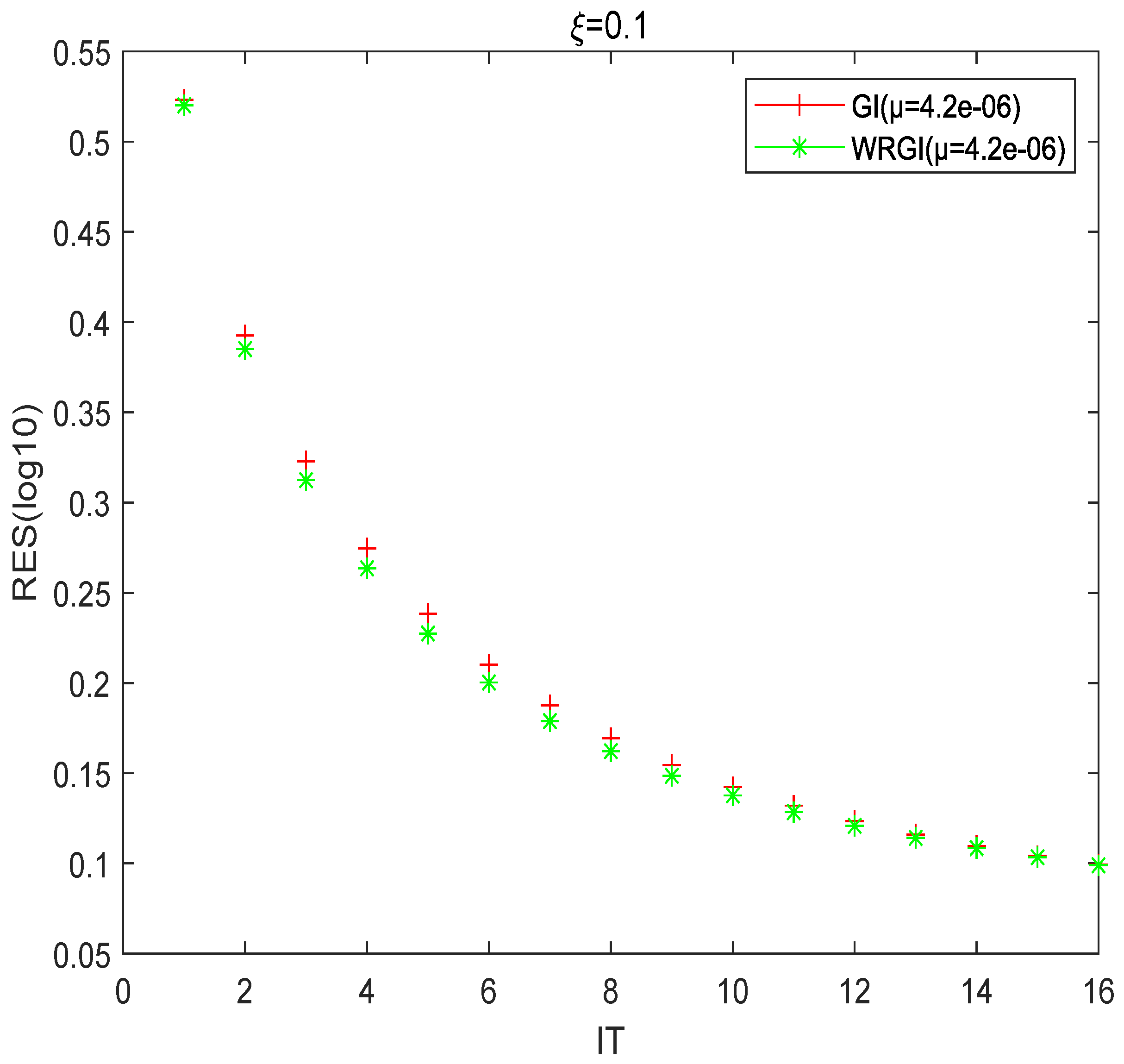
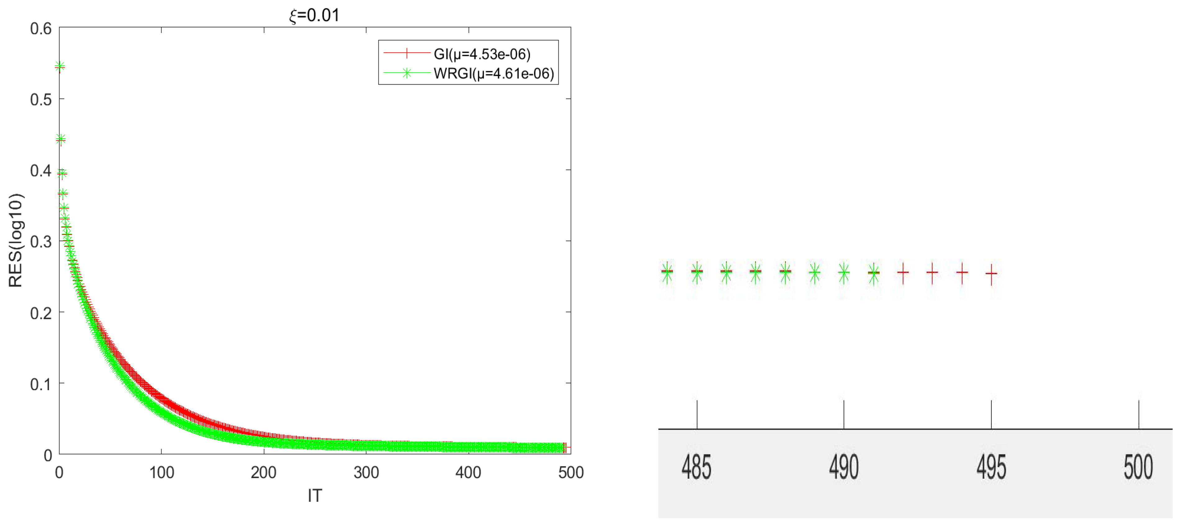
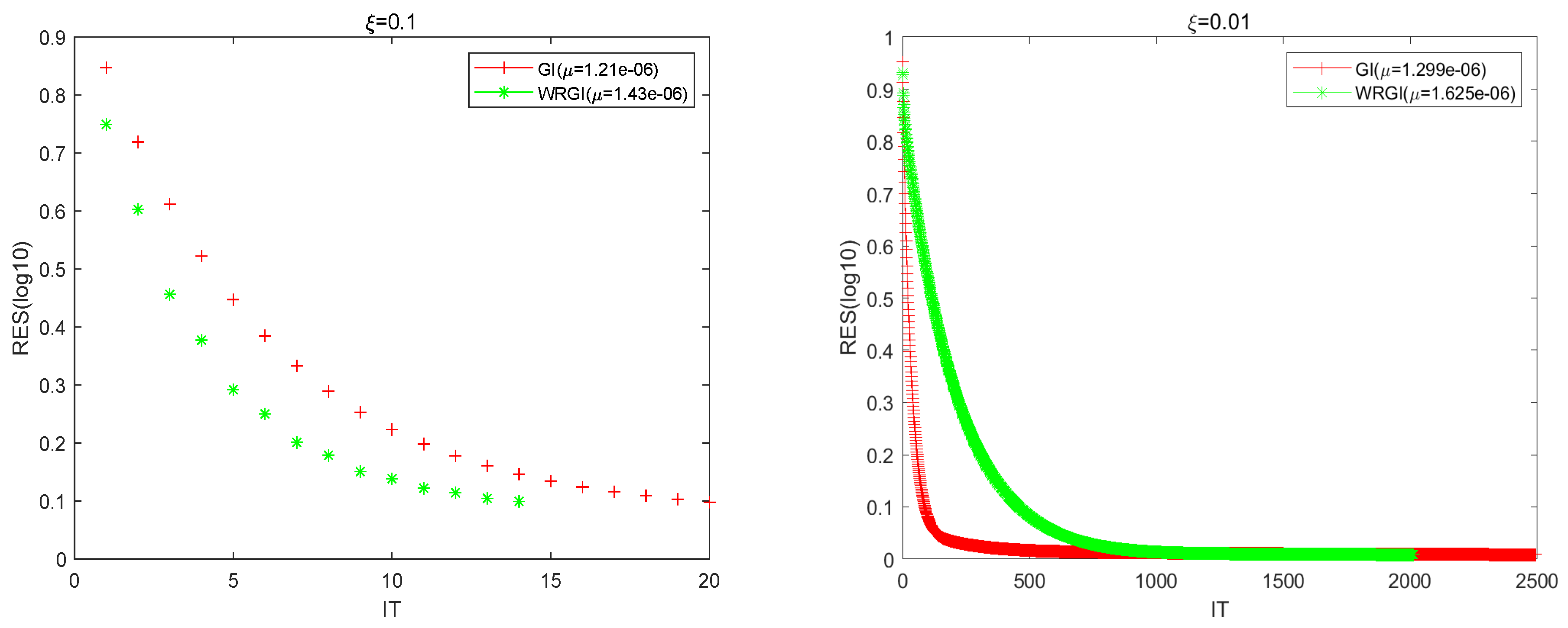
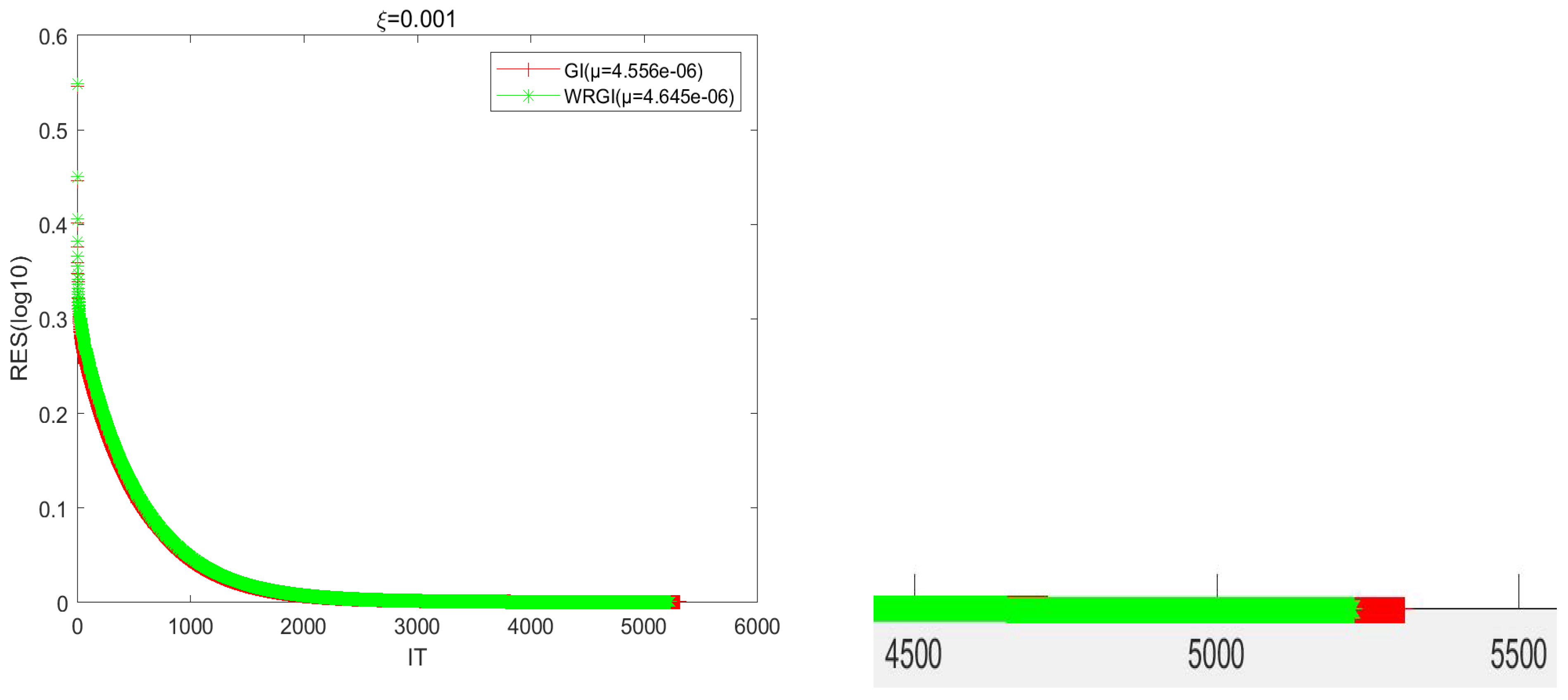
To better validate the advantage of the WRGI algorithm, Figure 1, Figure 2, Figure 3 and Figure 4 describe the convergence curves of the GI and WRGI algorithms for four different values of $\xi$. These curves reflect that the WRGI algorithm is convergent and its convergence speed is faster than the GI one, except for the case of $\xi =0.1$. Additionally, the advantage of the WRGI algorithm becomes more pronounced as the value of $\xi$ decreases. This is consistent with the results in Table 1.

Example 2.

We consider the generalized coupled conjugate and transpose Sylvester matrix equations

$$\left\{\begin{array}{c}{A}_{11}{X}_1{B}_{11}+C_{11}\overline{X_1}{D}_{11}+E_{12}{X}_2^T{F}_{12}+G_{12}{X}_2^H{H}_{12}=M_1,\\ A_{21}{X}_1{B}_{21}+C_{21}\overline{X_1}{D}_{21}+E_{22}{X}_2^T{F}_{22}+G_{22}{X}_2^H{H}_{22}=M_2,\end{array}\right.$$

with the coefficient matrices

$$\begin{array}{c}{A}_{11}=\left[\begin{array}{ccc}12& 5& 3\\ 19& 8& 2\\ -9& -3& 21\end{array}\right],B_{11}=\left[\begin{array}{ccc}-11& 23& 30\\ 4& -9& 3\\ 1& -35& 20\end{array}\right],C_{11}=\left[\begin{array}{ccc}8+1i& 1+21i& 7\\ -1+8i& 1& 26\\ 1i& 8& 41i\end{array}\right],\hfill \\ D_{11}=\left[\begin{array}{ccc}1& -1i& 1\\ 1i& 1& 1\\ 2& 1i& 1\end{array}\right],E_{12}=\left[\begin{array}{ccc}1& 1i& 1\\ 2i& 1& 0\\ 0& 1& 1\end{array}\right],F_{12}=\left[\begin{array}{ccc}1& 1& 6\\ 1& 0& 0\\ 0& 1& 1\end{array}\right],\hfill \\ G_{12}=\left[\begin{array}{ccc}1& 0& -1\\ 1& 4& 1\\ -2& 0& -2\end{array}\right],H_{12}=\left[\begin{array}{ccc}1& 0& -1\\ 0& 1i& 0\\ -1& 0& 1\end{array}\right],A_{21}=\left[\begin{array}{ccc}1& 0& 5i\\ 35& -1& 45\\ 1& -1& 1\end{array}\right],\hfill \\ B_{21}=\left[\begin{array}{ccc}-1+4i& 28& 1\\ 1& -42& 1\\ 1& 33& -3\end{array}\right],C_{21}=\left[\begin{array}{ccc}1i& 0& 1\\ -1& 1& -2\\ 0& 2& 1\end{array}\right],D_{21}=\left[\begin{array}{ccc}1& -1i& 3\\ 1& 1& 1\\ 1i& 1i& 1\end{array}\right],\hfill \\ E_{22}=\left[\begin{array}{ccc}1& -1i& 1\\ 1i& 3& 4-2i\\ -1& 2& 1\end{array}\right],F_{22}=\left[\begin{array}{ccc}1& 8& 2\\ 1& 0& 0\\ 0& 1& -3\end{array}\right],G_{22}=\left[\begin{array}{ccc}1& 0& -1\\ 1& 2& 1\\ -2& 0& -2\end{array}\right]\hfill \\ H_{22}=\left[\begin{array}{ccc}1& 0& -1\\ -1& -1i& 1\\ -1& 2& 1\end{array}\right],M_1=\left[\begin{array}{ccc}-136-344& 1780-688i& 5777+2083i\\ -1508-670i& 1819-1450i& 8360+3079i\\ 199-1526i& 4844+2846i& -4882+2714i\end{array}\right],\hfill \\ M_2=\left[\begin{array}{ccc}-19-76i& -1004-949i& 3+166i\\ -1222+1753i& -31239+8414i& 2088+432i\\ -28+10i& -1133-147i& 69+5i\end{array}\right].\hfill \end{array}$$

The unique solution for these matrix equations is

$$X_1^{*}=\left[\begin{array}{ccc}12+2i\hfill & 23-2i\hfill & 1\hfill \\ 1\hfill & -8\hfill & 10i\hfill \\ 2+6i\hfill & 2+2i\hfill & -6\hfill \end{array}\right],X_2^{*}=\left[\begin{array}{ccc}1+2i\hfill & 2-3i\hfill & 3+4i\hfill \\ 2-4i\hfill & -6+3i\hfill & -3+2i\hfill \\ 1+1i\hfill & 2+2i\hfill & -1-2i\hfill \end{array}\right].$$

In this example, we chose

$$X_p^{\left(i\right)}\left(0\right)={10}^{-6}\times I_3,X_p\left(0\right)={10}^{-6}\times I_3,i\in \left[1,2\right],p\in \left[1,2\right],$$

as the initial matrices and took

$$RES=\sqrt{\frac{M_1\left(k\right)+M_2\left(k\right)}{M_1\left(0\right)+M_2\left(0\right)}}\le \xi$$

as the termination condition with a positive number ξ, where

$$M_1\left(k\right)={∥M_1-A_{11}{X}_1\left(k\right)B_{11}-C_{11}\overline{X_1\left(k\right)}{D}_{11}-E_{12}{X}_2^T\left(k\right)F_{12}-G_{12}{X}_2^H\left(k\right)H_{12}∥}^2$$

and

$$M_2\left(k\right)={∥M_2-A_{21}{X}_1\left(k\right)B_{21}-C_{21}\overline{X_1\left(k\right)}{D}_{21}-E_{22}{X}_2^T\left(k\right)F_{22}-G_{22}{X}_2^H\left(k\right)H_{22}∥}^2,$$

and the prescribed maximum iterative number was $k_{max}$ = 20,000, while $X_p\left(k\right)$ $(p=1,2)$ denotes the kth iteration solution.

When ${\alpha }_1={\alpha }_2=0.5$, the WRGI algorithm degenerates into the GI one, and the optimal convergence factor calculated by Theorem 4 is $\mu =1.3151\times {10}^{-6}$. When ${\alpha }_1=0.6$ or ${\alpha }_2=0.4$, the optimal parameter of the WRGI algorithm is $\mu =1.6269\times {10}^{-6}$ in light of Theorem 4. Due to the existence of computation errors, as in Example 1, the parameters used in the GI and WRGI algorithms for Example 2 are the experimentally found optimal ones which minimize the IT of the tested algorithms. Through experimental debugging, the experimental optimal parameters of the GI algorithm were ${\mu }_{GI1}=1.21\times {10}^{-6}$ and ${\mu }_{GI2}=1.299\times {10}^{-6}$ for $\xi =0.1$ and $\xi =0.01$, respectively. And when ${\alpha }_1=0.6$ and ${\alpha }_2=0.4$, the experimental optimal parameters of the WRGI algorithm were ${\mu }_{WRGI1}=1.43\times {10}^{-6}$ and ${\mu }_{WRGI2}=1.625\times {10}^{-6}$ for $\xi =0.1$ and $\xi =0.01$, respectively.

In

Table 2. Numerical results of the tested algorithms for Example 2 with different values of $\xi$.

Algorithm		$\mathit{\xi }$
		0.1	0.01
GI	IT	21	2495
	CPU	0.0482	0.4058
	RES	$9.82\times {10}^{-2}$	$1.00\times {10}^{-2}$
WRGI	IT	15	2014
	CPU	0.0179	0.2831
	RES	$9.997\times {10}^{-2}$	$1.00\times {10}^{-2}$

, we compare the numerical results of the GI and WRGI algorithms to solve the generalized coupled conjugate and transpose Sylvester matrix equations in Example 2 with respect to two different values of ξ. Since the IT of the algorithms exceeded the maximum number of iterations when $\xi =0.001$ and $\xi =0.0001$, we did not list the corresponding numerical results here. From the numerical results listed in Table 2, we can conclude that when the value of ξ decreases, the IT and CPU times of the tested algorithms increase. The changing scope of the IT of the proposed WRGI algorithm was smaller than that for the GI one. In addition, the WRGI algorithm outperformed the GI one from the point of view of computing efficiency, and the advantage of the WRGI algorithm became more pronounced as ξ became small.

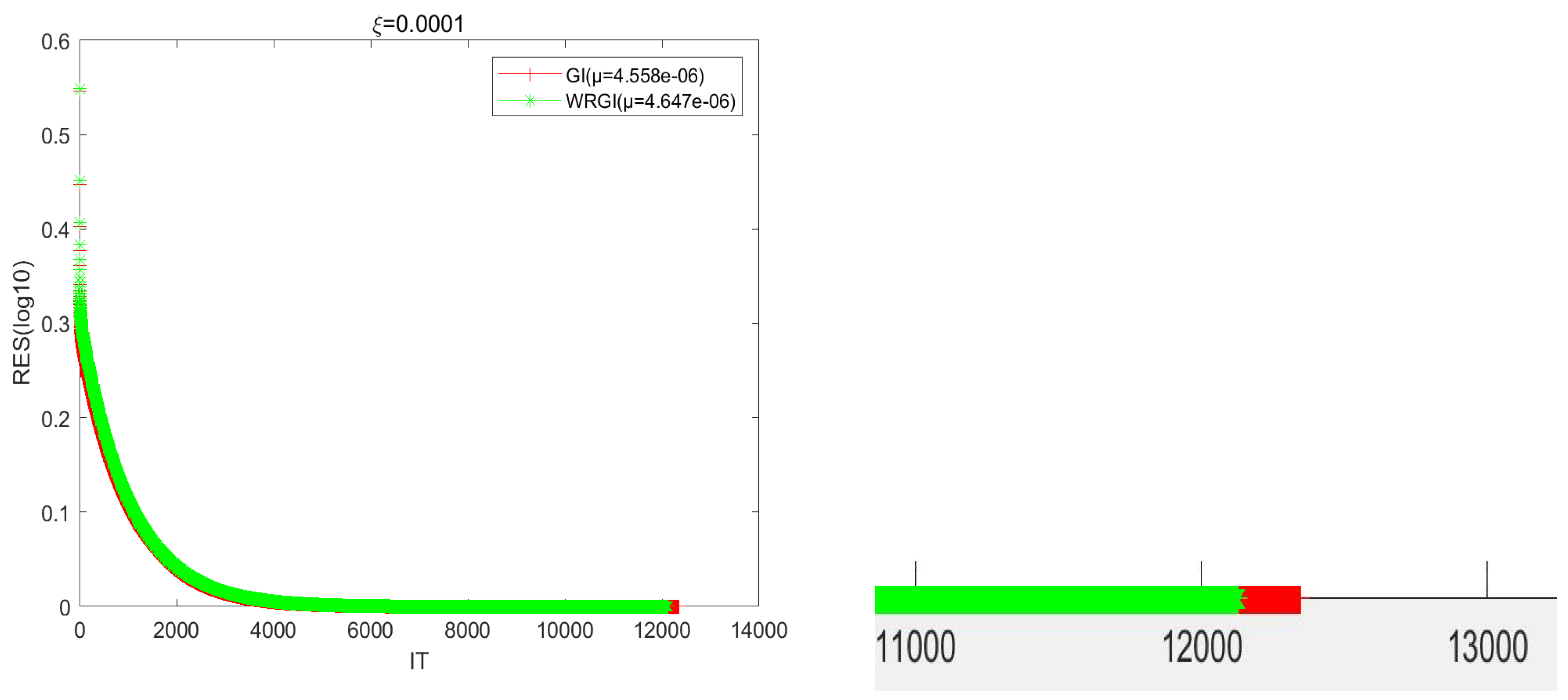
Figure 5 describes the convergence curves of the GI and WRGI algorithms for Example 2 with $\xi =0.1$ and $\xi =0.01$, respectively. It follows from Figure 5 that the error curves of the WRGI algorithm decreased faster than those for the GI one, which means that the proposed WRGI algorithm is superior to the GI one in terms of IT.

5. Concluding Remarks

In this work, by applying the weighted technique and introducing several relaxation factors into the GI algorithm, the weighted, relaxed gradient-based iterative (WRGI) algorithm was constructed for the generalized coupled conjugate and transpose Sylvester matrix equations. By using the real representation of a complex matrix and the vector-stretching operator, the necessary and sufficient conditions for the convergence of the WRGI algorithm were given, and its optimal convergence factor was settled theoretically. Finally, two numerical examples were offered to show the effectiveness and superiority of the proposed WRGI algorithm.

Note that only one step size factor μ is used in the WRGI algorithm. We will consider to adopt different step size factors in the WRGI algorithm and investigate its algebraic properties. Aside from that, establishing different versions of the WRGI algorithm and their convergent conditions when the system matrix is of a full-row rank, full-column rank or reduced rank deserve to be studied in our future work.

References

1. Fletcher, L.R.; Kuatslcy, J.; Nichols, N.K. Eigenstructure assignment in descriptor systems. IEEE Trans. Autom. Control. 1986, 31, 1138–1141. [Google Scholar] [CrossRef]
2. Zhou, B.; Zheng, W.-X.; Duan, G.-R. Stability and stabilization of discrete-time periodic linear systems with actuator saturation. Automatica 2011, 47, 1813–1820. [Google Scholar] [CrossRef]
3. Zhou, B.; Duan, G.-R. Periodic Lyapunov equation based approaches to the stabilization of continuous-time periodic linear systems. IEEE Trans. Autom. Control 2012, 57, 2139–2146. [Google Scholar] [CrossRef]
4. Ding, F.; Wang, F.-F.; Xu, L.; Wu, M.-H. Decomposition based least squares iterative identification algorithm for multivariate pseudo-linear ARMA systems using the data filtering. J. Frankl. Inst. 2017, 354, 1321–1339. [Google Scholar] [CrossRef]
5. Lv, L.-L.; Chen, J.-B.; Zhang, L.; Zhang, F.-R. Gradient-based neural networks for solving periodic Sylvester matrix equations. J. Frankl. Inst. 2022, 359, 10849–10866. [Google Scholar] [CrossRef]
6. Bai, Z.-Z.; Guo, X.-X.; Yin, J.-F. On two iteration methods for the quadratic matrix equations. Int. J. Numer. Anal. Model. 2005, 2, 114–122. [Google Scholar]
7. Bai, Z.-Z.; Guo, X.-X.; Xu, S.-F. Alternately linearized implicit iteration methods for the minimal nonnegative solutions of the nonsymmetric algebraic Riccati equations. Numer. Linear Algebra Appl. 2006, 13, 655–674. [Google Scholar] [CrossRef]
8. Bai, Z.-Z.; Huang, Y.-M.; Ng, M.K. On preconditioned iterative methods for Burgers equations. SIAM J. Sci. Comput. 2007, 29, 415–439. [Google Scholar] [CrossRef]
9. Dehghan, M.; Hajarian, M. An iterative algorithm for the reflexive solutions of the generalized coupled Sylvester matrix equations and its optimal approximation. Appl. Math. Comput. 2008, 202, 571–588. [Google Scholar]
10. Deng, Y.-B.; Bai, Z.-Z.; Gao, Y.-H. Iterative orthogonal direction methods for Hermitian minimum norm solutions of two consistent matrix equations. Numer. Linear Algebra Appl. 2006, 13, 801–823. [Google Scholar] [CrossRef]
11. Guo, K.-H.; Hu, X.-Y.; Zhang, L. A new iteration method for the matrix equation AX = B. Appl. Math. Comput. 2007, 187, 1434–1441. [Google Scholar]
12. Li, F.-L.; Gong, L.-S.; Hu, X.-Y.; Zhang, L. Successive projection iterative method for solving matrix AX = B. J. Comput. Appl. Math. 2010, 234, 2405–2410. [Google Scholar] [CrossRef]
13. Ding, F.; Chen, T.-W. On iterative solutions of general coupled matrix equations. Siam J. Control. Optim. 2006, 44, 2269–2284. [Google Scholar] [CrossRef]
14. Chen, Z.-B.; Chen, X.-S. Modification on the convergence results of the Sylvester matrix equation AX + XB = C. J. Frankl. Inst. 2022, 359, 3126–3147. [Google Scholar] [CrossRef]
15. Ramadan, M.A.; Bayoumi, A.M.E. A modified gradient-based algorithm for solving extended Sylvester-conjufate matrix equations. Asian J. Control. 2018, 20, 228–235. [Google Scholar] [CrossRef]
16. Zhang, J.-J. A note on the iterative solutions of general coupled matrix equation. Appl. Math. Comput. 2011, 217, 9380–9386. [Google Scholar] [CrossRef]
17. Zhang, H.-M. Reduced-rank gradient-based algorithms for generalized coupled Sylvester matrix equations and its applications. Comput. Math. Appl. 2015, 70, 2049–2062. [Google Scholar] [CrossRef]
18. Zhang, H.-M.; Yin, H.-C. Conjugate gradient least squares algorithm for solving the generalized coupled Sylvester matrix equations. Comput. Math. Appl. 2017, 73, 2529–2547. [Google Scholar] [CrossRef]
19. Wu, A.-G.; Feng, G.; Duan, G.-R.; Wu, W.-J. Iterative solutions to coupled Sylvester-conjugate matrix equations. Comput. Math. Appl. 2010, 60, 54–66. [Google Scholar] [CrossRef]
20. Huang, B.-H.; Ma, C.-F. Gradient-based iterative algorithms for generalized coupled Sylvester-conjugate matrix equations. Comput. Math. Appl. 2018, 75, 2295–2310. [Google Scholar] [CrossRef]
21. Huang, B.-H.; Ma, C.-F. The relaxed gradient-based iterative algorithms for a class of generalized coupled Sylvester-conjugate matrix equations. J. Frankl. Inst. 2018, 355, 3168–3195. [Google Scholar] [CrossRef]
22. Wang, W.-L.; Qu, G.-R.; Song, C.-Q. Cyclic gradient based iterative algorithm for a class of generalized coupled Sylvester-conjugate matrix equations. J. Frankl. Inst. 2023, 360, 7206–7229. [Google Scholar] [CrossRef]
23. Song, C.-Q.; Chen, G.-L.; Zhao, L.-L. Iterative solution to coupled Sylvester-transpose matrix equations. Appl. Math. Model. 2011, 35, 4675–4683. [Google Scholar] [CrossRef]
24. Huang, B.-H.; Ma, C.-F. On the relaxed gradient-based iterative methods for the generalized coupled Sylvester-transpose matrix equations. J. Frankl. Inst. 2022, 359, 10688–10725. [Google Scholar] [CrossRef]
25. Beik, F.P.A.; Salkuyeh, D.K.; Moghadam, M.M. Gradient-based iterative algorithm for solving the generalized coupled Sylvester-transpose and conjugate matrix equations over reflexive (anti-reflexive) matrices. Trans. Inst. Meas. Control. 2014, 36, 99–110. [Google Scholar] [CrossRef]
26. Wang, W.-L.; Song, C.-Q.; Ji, S.-P. Iterative solution to a class of complex matrix equations and its application in time-varying linear system. J. Appl. Math. Comput. 2021, 67, 317–341. [Google Scholar] [CrossRef]
27. Zhang, H.-M.; Yin, H.-C. New proof of the gradient-based iterative algorithm for a complex conjugate and transpose matrix equation. J. Frankl. Inst. 2017, 354, 7585–7603. [Google Scholar] [CrossRef]
28. Niu, Q.; Wang, X.; Lu, L.-Z. A relaxed gradient based algorithm for solving Sylvester equations. Asian J. Control. 2011, 13, 461–464. [Google Scholar] [CrossRef]
29. Wang, W.-L.; Song, C.-Q. Iterative algorithms for discrete-time periodic Sylvester matrix equations and its application in antilinear periodic system. Appl. Numer. Math. 2021, 168, 251–273. [Google Scholar] [CrossRef]
30. Wu, A.-G.; Zhang, Y.; Qian, Y.-Y. Complex Conjugate Matrix Equations; Science Press: Beijing, China, 2017. [Google Scholar]
31. Khalil, I.S.; Doyle, J.C.; Glover, K. Robust and Optimal Control; Prentice Hall: Hoboken, NJ, USA, 1996. [Google Scholar]
32. Zhang, H.-M. A finite iterative algorithm for solving the complex generalized coupled Sylvester matrix equations by using the linear operators. J. Frankl. Inst. 2017, 354, 1856–1874. [Google Scholar] [CrossRef]
Figure 1. Convergence curves of the tested algorithms for Example 1 with ξ = 0.1 .
Axioms 12 01062 g001
Figure 2. Convergence curves of the tested algorithms for Example 1 with ξ = 0.01 .
Axioms 12 01062 g002
Figure 3. Convergence curves of the tested algorithms for Example 1 with ξ = 0.001 .
Axioms 12 01062 g003
Figure 4. Convergence curves of the tested algorithms for Example 1 with ξ = 0.0001 .
Axioms 12 01062 g004
Figure 5. Convergence curves of the tested algorithms for Example 2 with ξ = 0.1 (left) and ξ = 0.01 (right).
Axioms 12 01062 g005