Numerical Simulation of Constrained Flows through Porous Media Employing Glimm’s Scheme

Abstract

This work uses a mixture theory approach to describe kinematically constrained flows through porous media using an adequate constitutive relation for pressure that preserves the problem hyperbolicity even when the flow becomes saturated. This feature allows using the same mathematical tool for handling unsaturated and saturated flows. The mechanical model can represent the saturated–unsaturated transition and vice-versa. The constitutive relation for pressure is a continuous and differentiable function of saturation: an increasing function with a strictly convex, increasing, and positive first derivative. This significant characteristic permits the fluid to establish a tiny controlled supersaturation of the porous matrix. The associated Riemann problem’s complete solution is addressed in detail, with explicit expressions for the Riemann invariants. Glimm’s semi-analytical scheme advances from a given instant to a subsequent one, employing the associated Riemann problem solution for each two consecutive time steps. The simulations employ a variation in Glimm’s scheme, which uses the mean of four independent sequences for each considered time, ensuring computational solutions with reliable positions of rarefaction and shock waves. The results permit verifying this significant characteristic.

1. Introduction

Transport phenomena in porous media present several relevant engineering applications, including problems that impact energy self-sufficiency and the environment. Among the examples, there are underground flows. They may contain various contaminants picked up from seepage and soil percolation. Another pertinent phenomenon is related to oil extraction, including enhanced oil recovery. Other examples are soil contamination by toxic waste or nuclear waste storage in deep rocky layers or the deep ocean seabed [1,2,3,4,5,6,7,8,9,10].

The motion strongly depends on saturation in flows through unsaturated porous media, and a force dependent on the saturation gradient mainly originates the fluid flow. These flows have been highly studied for about a century [11]; most use a volume average technique introduced by Whitaker [12] and analyzed by Alazmi and Vafai [13], combined with a continuum mechanics approach. Highly deformable porous media are handled using consolidation models based on Biot’s theory [14] and multi-scale models(a hierarchy from micro-scales to macro-scales, e.g., [15]). This work used a distinct approach: a continuum theory of mixtures. The mixture comprises continuous constituents simultaneously occupying the whole volume [16,17]. This viewpoint studies unsaturated fluid flow through porous media, considering a transition from unsaturated to saturated flow and vice versa. The unsaturated porous matrix is considered a three-constituent mixture composed of one solid constituent (porous matrix), one liquid constituent (conveniently called the fluid), and one gas constituent. This third constituent inclusion allows the consideration of the mixture’s compressibility, assuming it to be a very-low-density gas.

The dominance of normal stresses in these flows through porous media was suggested by Allen [18], reducing the partial stress tensor to a stress proportional to pressure. In this work, a continuous and differentiable constitutive relation as a function of the fluid fraction represents pressure: an increasing function, its first derivative being a strictly convex increasing, and positive function. This relation can impose an upper limit on the fluid fraction. In the vicinity of this upper limit, the fluid experienced high-pressure values, corresponding to an increase in the resistance of the porous matrix to a more significant fluid inflow. This constitutive relation ensures that the system remains hyperbolic even when the porous matrix becomes saturated.

Systems of parabolic or elliptic partial differential equations appropriately describe most transport phenomena, generally admitting regular solutions. Well-known numerical methods can implement their simulations. Since a finite velocity can characterize the propagation of any information in transport phenomena, hyperbolic systems allow a more realistic description of many phenomena. However, these systems may not admit regular solutions, requiring the generalization of the space of permissible solutions to include discontinuous solutions, which can involve shock waves.

Martins-Costa et al. [19] studied three distinct one-dimensional fluid flow geometries through unsaturated porous media using a mixture theory description. The constitutive relation used for the pressure allowed explicit closed equations to represent the Riemann invariants, leading to the complete solution of the associated Riemann problem [20]. This Riemann problem allows building a numerical solution using Glimm’s scheme [21] to handle the nonlinear system of hyperbolic equations. Glimm’s method is associated with an operator splitting procedure to consider the non-homogeneous portion of the differential equations.

Reference [22] proposed a restriction to the hyperbolic system to represent the filling of an unsaturated porous medium by a fluid employing a mixture theory description. The constitutive relation used for the pressure accounts for the upper bound arising from the rigid porous medium and the incompressible fluid assumptions. Previous work considered a geometric boundary preventing physically meaningless solutions throughout the porous medium, based on a pressure relation that is a one-sided geometrical constraint on the fluid fraction (see references therein). In [22], the fluid fraction unilateral geometric restriction was imposed solely in an appropriate vicinity of the porosity. The pressure and its first derivative are always continuous, and one can analytically calculate the associated Riemann invariants.

Martins-Costa et al. [23] proposed a model for pressure to analyze a liquid penetrating an unsaturated porous matrix, permitting a slight supersaturation. In [23], the authors used the mathematically imposed unilateral geometrical constraint, ensuring that the maximum value reached by the fluid fraction is the porosity and the saturation upper bound—the transition from unsaturated to saturated flow from previous work (see references therein). The model in [23] identifies the transition from unsaturated to saturated flow and vice versa, enabling the problem to remain hyperbolic, even when the flow becomes saturated. Combining a splitting method (separating the original equation into two pieces at each time step) with Glimm’s methodology can simulate the problem. However, this proposed pressure relation has a weakness: it is a continuous but nondifferentiable function of the fluid fraction.

This work proposes a more realistic constitutive relation for pressure as a function of saturation, where the first derivative is no longer a discontinuous function. The pressure is continuous and differentiable with an increasing function as the first derivative. In this case, a minimal (controlled) supersaturation is allowed, accounting for some minimal deformation of the porous matrix and always preserving the problem’s hyperbolicity. It presents the solution via Glimm’s method (advancing in time through the solution of the associated Riemann problem). The implementation of Glimm’s scheme uses a strategy to provide solutions free from the randomness of the sign of the random number used, resulting from the methodology proposed by Chorin [24], which guarantees solutions with more reliable rarefaction and shock wave positions, showing a strong tendency to preserve symmetry.

Despite the simplifications, the one-dimensional flow model in a porous matrix used in this work can be considered a first approximation for relevant and usual practical situations in engineering, such as flows in oil reservoirs or soil contamination by pollutants. The one-dimensional approach is reasonable when one of the flow directions has an order of magnitude greater than the others.

2. Mechanical Model

The three constituents’ mixture is chemically non-reacting without phase change, composed of a very slightly deformable solid constituent at rest, a fluid constituent (a Newtonian liquid), and a gas with negligible mass density, accounting for the mixture’s compressibility. Mass and momentum balance equations must be solved for the fluid constituent only, since the solid constituent is slightly deformable and the gas constituent ha negligible mass density [16,17]:

$$\begin{array}{l}\frac{\partial {\rho }_F}{\partial t}+\nabla \cdot ({\rho }_F{u}_F)=0\\ {\rho }_F\left[\frac{\partial u_F}{\partial t}+(\nabla u_F)u_F\right]=\nabla \cdot T_F+m_F+{\rho }_F{b}_F\end{array}$$

(1)

In Equation (1), the index ${}_F$ refers to the fluid constituent: ${\rho }_F$ is its mass density (the local ratio between its mass and the mixture volume), $u_F$ is its velocity, $T_F$ is the partial stress tensor (assumed to be symmetrical, so the angular momentum balance is automatically satisfied). Also, $m_F$ is the momentum source acting on the fluid constituent due to its interaction with the other mixtures’ constituents and $b_F$ is the body force per unit mass acting on it. To satisfy the momentum balance for the mixture, the sum of all momentum source terms must be zero.

The ratio between ${\rho }_F$ (fluid constituent mass density), ${\rho }_F$, and ${\rho }_f$ (fluid mass density, measured from a continuum mechanics viewpoint) defines the fluid fraction $\varphi$:

$$\varphi =\frac{{\rho }_F}{{\rho }_f}$$

(2)

Mixture theory allows kinematic independence among the constituents, requiring a source term to consider their dynamic interaction. This force is a momentum supply $m_F$, represented by two terms: the first one considers the drag effect of the solid constituent (porous matrix) on the fluid constituent (the Darcian term, adequately discussed by Srinivasan and Rajagopal [25]). The second term attempts to model capillary forces following a mixture theory approach, showing the strong dependency of motion on the saturation that characterizes unsaturated flows through porous media. Combining a splitting procedure with Glimm’s method allows for the simulation of the problem with the Darcian term, enabling one to account for homogeneous and non-homogeneous pieces of the hyperbolic system. However, this work neglected it. Martins-Costa and Saldanha da Gama [19] considered the effect of the Darcian term on flows through a porous matrix. This work used a splitting procedure to split away the non-homogeneous portion of the hyperbolic operator (time-evolutionary system) and Glimm’s method to solve the homogeneous associated problem. The purely time-evolutionary problem uses Glimm’s scheme solution as initial data.

$$m_F=-\frac{{\mu }_f}{K}{\varphi }^2{u}_F-\frac{{\mu }_f𝒟}{K}\nabla \varphi \hspace{1em}\Rightarrow \hspace{1em}{m}_F=-\frac{{\mu }_f𝒟}{K}\nabla \varphi$$

(3)

In Equation (3), ${\mu }_f$ is the viscosity of the fluid and $K$ is the specific permeability of the porous medium, both measured following a continuum mechanics approach. Also, $𝒟$ represents a diffusion coefficient.

The constitutive equation for the partial stress tensor acting on the fluid constituent (analogous to the Cauchy stress tensor in Continuum Mechanics), assuming dominance of normal stresses over shear stresses and interphase tractions [18], is given by:

$$T_F=-\hspace{0.17em}\varphi \hspace{0.17em}\overline{p}\hspace{0.17em}1$$

(4)

with $\overline{p}$ being a pressure and $1$ being the identity tensor.

Combining the balance Equation (1) with the constitutive assumptions presented in Equations (3) and (4), and supposing dependency on position x and on time t only. Also, assuming that the velocity in the flow direction u is the only non-vanishing component of $u_F$, and the absence of body forces affecting the flow direction, the problem is expressed as:

$$\begin{array}{l}\frac{\partial \varphi }{\partial t}+\frac{\partial }{\partial x}\left(\varphi u\right)=0\\ {\rho }_f\left[\varphi \frac{\partial u}{\partial t}+\varphi u\frac{\partial u}{\partial x}\right]=-\frac{\partial }{\partial x}\left(\varphi \overline{p}\right)-\frac{{\rho }_f^{}{\mu }_f𝒟}{K}\frac{\partial \varphi }{\partial x}\end{array}$$

(5)

Employing a reference pressure $\stackrel{⌣}{p}$ allows for a convenient redefinition of the pressure, such that:

$$\stackrel{⌣}{p}\frac{\partial \varphi }{\partial x}=\frac{\partial }{\partial x}\left(\varphi \overline{p}\right)+\frac{{\rho }_f^{}{\mu }_f𝒟}{K}\frac{\partial \varphi }{\partial x}$$

(6)

Using the pressure redefinition given by Equation (6) permits writing the nonlinear system (5) as a nonlinear homogeneous hyperbolic system:

$$\begin{array}{l}\frac{\partial \varphi }{\partial t}+\frac{\partial }{\partial x}\left(\varphi u\right)=0\\ \frac{\partial }{\partial t}\left(\varphi u\right)+\frac{\partial }{\partial x}\left(\stackrel{⌣}{p}+\varphi u^2\right)=0\end{array}$$

(7)

3. Constitutive Relation

Before presenting the constitutive assumption for pressure, it is convenient to define saturation as:

$$\psi =\frac{\varphi }{\epsilon }$$

(8)

where $\epsilon$ is the porosity. Saturation is, originally, less than or equal to one.

Nevertheless, in this paper, a “super-saturation” is allowed to take into account some small deformation of the porous medium and preserve the hyperbolic behavior of the system of equations.

In other words, the following is allowed:

$$0\le \psi =\frac{\varphi }{\epsilon }<1+\frac{\delta }{\epsilon },\hspace{1em}\delta <<\epsilon$$

(9)

in which $\delta$ is a tiny positive constant. The proposition in Equation (9) allows admitting a tiny supersaturation.

At this point, one can consider a relationship between pressure and saturation, allowing the introduction of the following constitutive equation for pressure:

$$p=\tilde{p}\left(\varphi \right)=\frac{\varphi }{\epsilon +\delta }+{\alpha }^2\frac{\varphi }{\epsilon +\delta -\varphi }-2\alpha \ln \left(\frac{\epsilon +\delta -\varphi }{\epsilon +\delta }\right),\hspace{1em}\alpha \ge 0$$

(10)

that can be rewritten as:

$$p=\widehat{p}\left(\phi \right)=\phi +{\alpha }^2\frac{\phi }{1-\phi }-2\alpha \ln \left(1-\phi \right),\hspace{1em}\alpha \ge 0$$

(11)

in which:

$$\phi =\frac{\varphi }{\epsilon +\delta }$$

(12)

where $p$ is a pressure proportional to $\stackrel{⌣}{p}$, defined in Equation (6), and the variable $\phi$ is, from now on, called saturation.

The constitutive relation presented in Equation (11) depends on saturation and a consistently positive parameter $\alpha$. This relation provides an upper bound for saturation, ensuring a reliable and always physically consistent simulation. The porous matrix’s minimal and controlled supersaturation is permitted, so the hyperbolicity is maintained irrespective of the fluid fraction value. The constitutive relation presented in Equation (11) bestows closed-form expressions for the Riemann invariants, as seen in the section describing the associated Riemann problem.

Combining the nonlinear homogeneous hyperbolic system (7) with the constitutive relation (11) results in the following nonlinear homogeneous hyperbolic system with saturation and velocity as unknowns:

$$\begin{array}{l}\frac{\partial \phi }{\partial t}+\frac{\partial }{\partial x}\left(\phi u\right)=0\\ \frac{\partial }{\partial t}\left(\phi u\right)+\frac{\partial }{\partial x}\left(p+\phi u^2\right)=0\\ p=\widehat{p}\left(\phi \right)=\phi +{\alpha }^2\frac{\phi }{1-\phi }-2\alpha \ln \left(1-\phi \right),\hspace{1em}\alpha \ge 0\end{array}$$

(13)

Even if the pressures become extremely large, the supersaturation presents an a priori limit:

$$\underset{p\to \infty }{\lim }\phi =1$$

(14)

The flow is said to be “saturated” in the regions where $\epsilon \le \varphi <\epsilon +\delta$. When $\varphi >\epsilon$ (supersaturated regions), the propagation speeds and pressure increase quickly for larger saturation values. The system of partial differential equations is always hyperbolic, presenting a realistic response.

4. The Associated Riemann Problem

The hyperbolic system presented in Equation (13) can be written in a more convenient form:

$$\mathrm{P}\frac{\partial }{\partial t}\left[\begin{array}{c}\phi \\ \phi u\end{array}\right]+A\frac{\partial }{\partial x}\left[\begin{array}{c}\phi \\ \phi u\end{array}\right]=0,\hspace{1em}A=\left[\begin{array}{cc}0& 1\\ p\prime -u^2& 2u\end{array}\right],\hspace{1em}p\prime ={\left(1+\frac{\alpha }{1-\phi }\right)}^2$$

(15)

Consider the Cauchy problem given by:

$$\begin{array}{l}\frac{\partial \phi }{\partial t}+\frac{\partial }{\partial x}\left(\phi u\right)=0\\ \frac{\partial }{\partial t}\left(\phi u\right)+\frac{\partial }{\partial x}\left(\phi u^2+p\right)=0\\ \left(\phi ,u\right)=\left\{\begin{array}{c}({\phi }_L,u_L),\hspace{1em}-\infty <x<0,\hspace{1em}t=0\\ ({\phi }_R,u_R),\hspace{1em}0<x<\infty ,\hspace{1em}t=0\end{array} \right.\end{array}$$

(16)

in which ${\phi }_L$ and ${\phi }_R$ are positive valued constants. Problem (16) is a Riemann problem [20], and its solution (in a generalized space of allowable solutions) is subjected solely to the ratio $x/t$. In other words, the following system represents (13):

$$\begin{array}{l}\frac{d\phi }{d\eta }\frac{\partial \eta }{\partial t}+\frac{d}{d\eta }\left(\phi u\right)\frac{\partial \eta }{\partial x}=0\hspace{1em}\\ \frac{d}{d\eta }\left(\phi u\right)\frac{\partial \eta }{\partial t}+\frac{d}{d\eta }\left(\phi u^2+p\right)\frac{\partial \eta }{\partial x}=0\end{array}$$

(17)

employing a similarity variable such that:

$$\eta =x/t\hspace{1em}\Rightarrow \hspace{1em}\frac{\partial \eta }{\partial t}=-\frac{1}{t}\eta ;\hspace{1em}\frac{\partial \eta }{\partial x}=\frac{1}{t}$$

(18)

In this way, (15) becomes:

$$\left[\begin{array}{cc}-\eta & 1\\ p\prime -u^2& 2u-\eta \end{array}\right]\left[\begin{array}{c}\underset{}{d\phi }\\ \stackrel{}{d\left(\phi u\right)}\end{array}\right]=0$$

(19)

To satisfy the nonlinear problem (15), either $\phi$ and $u$ must be constants, or $\eta =\lambda$ ($\lambda \to$ eigenvalue of $A$ and $\left(d\phi ,d\left(\phi u\right)\right)\to$ eigenvector).

The eigenvalues of the matrix $A$, defined in Equation (15), in increasing order, are given by:

$${\lambda }_1=u-1-\frac{\alpha }{1-\phi } \mathrm{and} {\lambda }_2=u+1+\frac{\alpha }{1-\phi }$$

(20)

The equation below allows for obtaining the associated eigenvectors:

$$\left(u-1-\frac{\alpha }{1-\phi }\right)d\phi -d\left(\phi u\right)=0 \mathrm{and} \left(u+1+\frac{\alpha }{1-\phi }\right)d\phi -d\left(\phi u\right)=0$$

(21)

Taking into account Equation (21) allows obtaining the following equations:

$$\begin{array}{l}{\displaystyle \int \left(\frac{1}{\phi }+\frac{\alpha }{\phi \left(1-\phi \right)}\right)d\phi }+u=constant\hspace{1em}(associated to {\lambda }_1)\\ -{\displaystyle \int \left(\frac{1}{\phi }+\frac{\alpha }{\phi \left(1-\phi \right)}\right)d\phi }+u=constant\hspace{1em}(associated to {\lambda }_2)\end{array}$$

(22)

or, in an alternative form,

$$\ln \phi +\alpha \ln \left(\frac{\phi }{1-\phi }\right)+\frac{\alpha }{1-\phi }+{\lambda }_1=constant\hspace{1em}(associated to {\lambda }_1)$$

(23)

$$-\ln \phi -\alpha \ln \left(\frac{\phi }{1-\phi }\right)-\frac{\alpha }{1-\phi }+{\lambda }_2=constant\hspace{1em}(associated to {\lambda }_2)$$

(24)

Since $\phi \in \left(0,1\right)$,

$$\frac{d}{d\phi }\left\{\ln \phi +\alpha \ln \left(\frac{\phi }{1-\phi }\right)+\frac{\alpha }{1-\phi }\right\}=\frac{1}{\phi }+\frac{\alpha }{\phi }+\frac{\alpha }{1-\phi }+\frac{\alpha }{{\left(1-\phi \right)}^2}>0$$

(25)

Since the eigenvalues correspond to the similarity variable $\eta$, two states,$\left({\phi }_1,u_1\right)$ and $\left({\phi }_2,u_2\right)$, are connected by a continuous function of $\eta$ satisfying Equation (23) if, and only if, $\phi$ decreases as ${\lambda }_1$ increases, and this connection is called a 1-rarefaction. On the other hand, two states ($\left({\phi }_1,u_1\right)$ and $\left({\phi }_2,u_2\right)$) are connected by a continuous function of $\eta$ satisfying Equation (24) if, and only if, $\phi$ increases as ${\lambda }_2$ increases, and this connection is called a 2-rarefaction. In these cases, the functional relationship between $\phi$ and $\eta$ is obtained from Equation (23) or Equation (24) by replacing the considered eigenvalue with $\eta$. Equation (22) allows obtaining the function $u$.

Now, it is opportune to return to the hyperbolic system represented in a convenient form, (15). A constant left state $\left({\phi }_L,u_L\right)$ connected to a constant state $\left({\phi }_{\ast },u_{\ast }\right)$, employing a continuous function of $\eta$, with ${\lambda }_{1L}<{\lambda }_{1\ast }$, must satisfy:

$$\ln {\phi }_L+\alpha \ln \left(\frac{{\phi }_L}{1-{\phi }_L}\right)+u_L=\ln {\phi }_{\ast }+\alpha \ln \left(\frac{{\phi }_{\ast }}{1-{\phi }_{\ast }}\right)+u_{\ast },\hspace{1em}with\hspace{1em}{\phi }_L>{\phi }_{\ast }$$

(26)

On the other hand, to connect the constant state $\left({\phi }_R,u_R\right)$ to a constant state $\left({\phi }_{\ast },u_{\ast }\right)$, employing a continuous function of $\eta$, with ${\lambda }_{2R}>{\lambda }_{2\ast }$, the following relation must be satisfied:

$$-\ln {\phi }_R-\alpha \ln \left(\frac{{\phi }_R}{1-{\phi }_R}\right)+u_R=-\ln {\phi }_{\ast }-\alpha \ln \left(\frac{{\phi }_{\ast }}{1-{\phi }_{\ast }}\right)+u_{\ast },\hspace{1em}with\hspace{1em}{\phi }_R>{\phi }_{\ast }$$

(27)

Since (25) holds, the solution to problem (16) consists of connecting the states $\left({\phi }_L,u_L\right)$ and $\left({\phi }_R,u_R\right)$ to an intermediate state $\left({\phi }_{\ast },u_{\ast }\right)$ through continuous functions of the similarity variable $\eta$.

So, in this case, once $\left({\phi }_L,u_L\right)$ and $\left({\phi }_R,u_R\right)$ are given,$\left({\phi }_{\ast },u_{\ast }\right)$ is obtained from the system combining Equations (26) and (27), in which ${\phi }_{\ast }$ and $u_{\ast }$ are the unique solutions of the following system:

$$\begin{array}{l}{u}_{\ast }=\frac{1}{2}\left(\ln \frac{{\phi }_L}{{\phi }_R}+\alpha \ln \left(\frac{{\phi }_L\left(1-{\phi }_R\right)}{{\phi }_R\left(1-{\phi }_L\right)}\right)+u_L+u_R\right)\\ \ln {\phi }_{\ast }+\alpha \ln \left(\frac{{\phi }_{\ast }}{1-{\phi }_{\ast }}\right)=\frac{1}{2}\left(\ln \left({\phi }_L{\phi }_R\right)+\alpha \ln \left(\frac{{\phi }_L{\phi }_R}{\left(1-{\phi }_L\right)\left(1-{\phi }_R\right)}\right)+u_L-u_R\right)\end{array}$$

(28)

Now, it is appropriate to define the (invertible) function of saturation $F=\widehat{F}\left(\phi \right)$ and its inverse as:

$$F=\widehat{F}\left(\phi \right)=\ln \phi +\alpha \ln \left(\frac{\phi }{1-\phi }\right)+\frac{\alpha }{1-\phi },\hspace{1em}f=\widehat{f}\left(\widehat{F}\left(\phi \right)\right)=\phi ,\hspace{1em}\hspace{1em}0<\phi <1$$

(29)

The solution in this case may be represented by:

$$\begin{array}{l}\phi =\left\{\begin{array}{c}{\phi }_L,\hspace{1em}-\infty <\eta \le {\lambda }_{1L}\\ \widehat{f}\left(\widehat{F}\left({\phi }_L\right)+{\lambda }_{1L}-\eta \right),\hspace{1em}{\lambda }_{1L}<\eta <{\lambda }_{1\ast }\\ {\phi }_{\ast },\hspace{1em}{\lambda }_{1\ast }\le \eta \le {\lambda }_{2\ast }\\ \widehat{f}\left(\widehat{F}\left({\phi }_R\right)-{\lambda }_{1R}+\eta \right),\hspace{1em}{\lambda }_{2\ast }<\eta <{\lambda }_{2R}\\ {\phi }_R,\hspace{1em}{\lambda }_{2R}\le \eta <\infty \end{array}\right.\\ u=\left\{\begin{array}{c}{u}_L,\hspace{1em}-\infty <\eta \le {\lambda }_{1L}\\ \left(\alpha +1\right)\ln \left(\frac{{\phi }_L}{\phi }\right)-\alpha \ln \left(\frac{1-{\phi }_L}{1-\phi }\right)+u_L,\hspace{1em}{\lambda }_{1L}<\eta <{\lambda }_{1\ast }\\ u_{\ast },\hspace{1em}{\lambda }_{1\ast }\le \eta \le {\lambda }_{2\ast }\\ -\left(\alpha +1\right)\ln \left(\frac{{\phi }_R}{\phi }\right)+\alpha \ln \left(\frac{1-{\phi }_R}{1-\phi }\right)+u_R,\hspace{1em}{\lambda }_{2\ast }<\eta <{\lambda }_{2R}\hspace{1em}\\ u_R,\hspace{1em}{\lambda }_{2R}\le \eta <\infty \end{array}\right.\end{array}$$

(30)

in which:

$$\begin{array}{l}{\lambda }_{1L}=u_L-\left(1+\frac{\alpha }{1-{\phi }_L}\right);\hspace{1em}{\lambda }_{1\ast }=u_{\ast }-\left(1+\frac{\alpha }{1-{\phi }_{\ast }}\right)\\ {\lambda }_{2\ast }=u_{\ast }+\left(1+\frac{\alpha }{1-{\phi }_{\ast }}\right);\hspace{1em}{\lambda }_{2R}=u_R+\left(1+\frac{\alpha }{1-{\phi }_R}\right)\end{array}$$

(31)

This continuous solution is called a 1-rarefaction/2-rarefaction and takes place if, and only if,

$$u_R-u_L\ge \left|\ln \frac{{\phi }_L}{{\phi }_R}+\alpha \ln \left(\frac{{\phi }_L\left(1-{\phi }_R\right)}{{\phi }_R\left(1-{\phi }_L\right)}\right)\right|$$

(32)

When the equality holds, the connection is either a 1-rarefaction or a 2-rarefaction since the intermediate state coincides with the left state (in this case, there is only a 2-rarefaction) or with the right state (in this case, there is only a 1-rarefaction). In other words,

$$\begin{array}{l}\ln \frac{{\phi }_L}{{\phi }_R}+\alpha \ln \left(\frac{{\phi }_L\left(1-{\phi }_R\right)}{{\phi }_R\left(1-{\phi }_L\right)}\right)=u_R-u_L,\hspace{0.33em}\hspace{0.33em}with\hspace{1em}{\phi }_L>{\phi }_R\hspace{0.33em}\hspace{0.33em}\Rightarrow \hspace{0.33em}\hspace{0.33em}{\phi }_R={\phi }_{\ast }\to \hspace{0.33em}\hspace{0.33em}1-rarefaction\\ \ln \frac{{\phi }_R}{{\phi }_L}+\alpha \ln \left(\frac{{\phi }_R\left(1-{\phi }_L\right)}{{\phi }_L\left(1-{\phi }_R\right)}\right)=u_R-u_L,\hspace{0.33em}\hspace{0.33em}with\hspace{1em}{\phi }_R>{\phi }_L\hspace{0.33em}\hspace{0.33em}\Rightarrow \hspace{0.33em}\hspace{0.33em}{\phi }_L={\phi }_{\ast }\to \hspace{0.33em}\hspace{0.33em}2-rarefaction\end{array}$$

(33)

Nevertheless, initial data satisfying the continuous solutions given by Equation (32) cannot always adequately represent the problem. Consequently, the space of permissible solutions must be expanded to allow for discontinuous solutions.

These discontinuous solutions are constructed by connecting two states by a discontinuity. They must satisfy the entropy conditions [20,26,27,28] and the Rankine–Hugoniot jump conditions [20,26,29,30,31]. The jump conditions associated with the nonlinear hyperbolic system (15) are given by:

$$\frac{\left[\phi u\right]}{\left[\phi \right]}=\frac{\left[\phi u^2+p\right]}{\left[\phi u\right]}=s$$

(34)

in which $\left[•\right]$ denotes the “jump” of “$•$”.

Since (25) holds, for any two states that a continuous function cannot connect, a shock links them and satisfy the entropy conditions. Two states $\left({\phi }_1,u_1\right)$ and $\left({\phi }_2,u_2\right)$, connected by a shock, must satisfy the following:

$$\frac{{\phi }_2{u}_2-{\phi }_1{u}_1}{{\phi }_2-{\phi }_1}=\frac{{\phi }_2{u}_2^2-{\phi }_1{u}_1^2+p_2-p_1}{{\phi }_2{u}_2-{\phi }_1{u}_1}=s$$

(35)

in which $s$ is the shock speed, and $\eta =s$ is the shock position. As pointed out, to satisfy the entropy conditions, two states are linked by a shock if, and only if, a continuous function cannot connect them (a rarefaction coupling) [20,27,29,30,31].

A shock links the left state $\left({\phi }_L,u_L\right)$ to the constant state $\left({\phi }_{\ast },u_{\ast }\right)$ whenever ${\phi }_L<{\phi }_{\ast }$. This shock is called a 1-shock. The relationship between these two states is given by:

$$u_{\ast }-u_L=-\sqrt{\left(\frac{1}{{\phi }_L}-\frac{1}{{\phi }_{\ast }}\right)\left(p_{\ast }-p_L\right)},\hspace{1em}{\phi }_L<{\phi }_{\ast },\hspace{1em}{p}_{\ast }=\widehat{p}\left({\phi }_{\ast }\right),\hspace{1em}{p}_L=\widehat{p}\left({\phi }_L\right)$$

(36)

The speed of the 1-shock, denoted by $s_1$, is given by:

$$s_1=\frac{{\phi }_{\ast }{u}_{\ast }-{\phi }_L{u}_L}{{\phi }_{\ast }-{\phi }_L}$$

(37)

The constant state $\left({\phi }_{\ast },u_{\ast }\right)$ links to the right state $\left({\phi }_R,u_R\right)$ by employing a shock called a 2-shock through the same protocol. If ${\phi }_R<{\phi }_{\ast }$, then the states $\left({\phi }_{\ast },u_{\ast }\right)$ and $\left({\phi }_R,u_R\right)$ are such that:

$$u_{\ast }-u_R=\sqrt{\left(\frac{1}{{\phi }_{\ast }}-\frac{1}{{\phi }_R}\right)\left(p_R-p_{\ast }\right)},\hspace{1em}{\phi }_R<{\phi }_{\ast },\hspace{1em}{p}_{\ast }=\widehat{p}\left({\phi }_{\ast }\right),\hspace{1em}{p}_R=\widehat{p}\left({\phi }_R\right)$$

(38)

The speed of the 2-shock, denoted by $s_2$,is given by:

$$s_2=\frac{{\phi }_R{u}_R-{\phi }_{\ast }{u}_{\ast }}{{\phi }_R-{\phi }_{\ast }}$$

(39)

Note that:

$$\begin{array}{l}{u}_L-u_R=\sqrt{\left(\frac{1}{{\phi }_L}-\frac{1}{{\phi }_R}\right)\left(p_R-p_L\right)},\hspace{1em}{\phi }_L<{\phi }_R\hspace{1em}\Rightarrow \hspace{1em}{\phi }_{\ast }={\phi }_R\hspace{1em}\to 1-shock\\ u_L-u_R=\sqrt{\left(\frac{1}{{\phi }_L}-\frac{1}{{\phi }_R}\right)\left(p_R-p_L\right)},\hspace{1em}{\phi }_R<{\phi }_L\hspace{1em}\Rightarrow \hspace{1em}{\phi }_{\ast }={\phi }_L\hspace{1em}\to 2-shock\hspace{1em}\end{array}$$

(40)

Table 1. Riemann problem possible solutions: conditions for saturation and velocity.

${\phi }_L>{\phi }_{\ast }<{\phi }_R$	→	1—rarefaction/2—rarefaction	→	$u_L<u_{\ast }<u_R$
${\phi }_L<{\phi }_{\ast }>{\phi }_R$	→	1—shock/2—shock	→	$u_L>u_{\ast }>u_R$
${\phi }_L>{\phi }_{\ast }>{\phi }_R$	→	1—rarefaction/2—shock	→	$u_L<u_{\ast }>u_R$
${\phi }_L<{\phi }_{\ast }<{\phi }_R$	→	1—shock/2—rarefaction	→	$u_L>u_{\ast }<u_R$
${\phi }_L={\phi }_{\ast }<{\phi }_R$	→	2—rarefaction	→	$u_L=u_{\ast }<u_R$
${\phi }_L>{\phi }_{\ast }={\phi }_R$	→	1—rarefaction	→	$u_L<u_{\ast }=u_R$
${\phi }_L={\phi }_{\ast }>{\phi }_R$	→	2—shock	→	$u_L=u_{\ast }>u_R$
${\phi }_L<{\phi }_{\ast }={\phi }_R$	→	1—shock	→	$u_L>u_{\ast }=u_R$

summarizes the possible solutions (rarefactions or shocks) for the Riemann problem (16) in a generalized sense concerning the conditions for saturation and velocity at the left, intermediate, and right states.

Table 2. Riemann problem solution: a priori choice.

1-rarefaction/ 2-rarefaction	$\iff$	$u_R-u_L\ge \left|\ln \left(\frac{{\phi }_L^{\alpha +1}{\left(1-{\phi }_R\right)}^{\alpha }}{{\phi }_R^{\alpha +1}{\left(1-{\phi }_L\right)}^{\alpha }}\right)\right|$
1-shock/ 2-shock	$\iff$	$u_R-u_L\le -\sqrt{\left(\frac{1}{{\phi }_R}-\frac{1}{{\phi }_L}\right)\left(p_L-p_R\right)}$
1-rarefaction/ 2-shock	$\iff$	$-\sqrt{\left(\frac{1}{{\phi }_R}-\frac{1}{{\phi }_L}\right)\left(p_L-p_R\right)}<u_R-u_L<\left|\ln \left(\frac{{\phi }_L^{\alpha +1}{\left(1-{\phi }_R\right)}^{\alpha }}{{\phi }_R^{\alpha +1}{\left(1-{\phi }_L\right)}^{\alpha }}\right)\right|,{\phi }_L>{\phi }_R$
1-shock/ 2-rarefaction	$\iff$	$-\sqrt{\left(\frac{1}{{\phi }_R}-\frac{1}{{\phi }_L}\right)\left(p_L-p_R\right)}<u_R-u_L<\left|\ln \left(\frac{{\phi }_L^{\alpha +1}{\left(1-{\phi }_R\right)}^{\alpha }}{{\phi }_R^{\alpha +1}{\left(1-{\phi }_L\right)}^{\alpha }}\right)\right|,{\phi }_L<{\phi }_R$

presents the conditions for the four possible solutions to the Riemann problem, showing the links by rarefactions and/or by shocks.

Note that when the intermediate state $\left({\phi }_{\ast },u_{\ast }\right)$ coincides with the left state $\left({\phi }_L,u_L\right)$, the solution will be a 2-rarefaction or a 2-shock. If the intermediate state $\left({\phi }_{\ast },u_{\ast }\right)$ coincides with the right state, the solution will be a 1-rarefaction or a 1-shock.

Equation (30) presents the complete solution for a 1-rarefaction/2-rarefaction. For a 1-shock/2-shock, the solution is given by:

$$\begin{array}{l}\phi =\left\{\begin{array}{c}{\phi }_L,\hspace{1em}-\infty <\eta <s_1\\ {\phi }_{\ast },\hspace{1em}{s}_1<\eta <s_2\\ {\phi }_R,\hspace{1em}{s}_2<\eta <\infty \end{array}\right.\\ u=\left\{\begin{array}{c}{u}_L,\hspace{1em}-\infty <\eta <s_1\\ u_{\ast },\hspace{1em}{s}_1<\eta <s_2\\ u_R,\hspace{1em}{s}_2<\eta <\infty \end{array}\right.\end{array}$$

(41)

in which ${\phi }_{\ast }$ and $u_{\ast }$ are obtained from:

$$\begin{array}{l}{u}_{\ast }-u_L=-\sqrt{\left(\frac{1}{{\phi }_L}-\frac{1}{{\phi }_{\ast }}\right)\left(p_{\ast }-p_L\right)},\hspace{1em}{\phi }_L<{\phi }_{\ast }\\ u_{\ast }-u_R=\sqrt{\left(\frac{1}{{\phi }_{\ast }}-\frac{1}{{\phi }_R}\right)\left(p_R-p_{\ast }\right)},\hspace{1em}{\phi }_R<{\phi }_{\ast }\\ \to \sqrt{\left(\frac{1}{{\phi }_L}-\frac{1}{{\phi }_{\ast }}\right)\left(p_{\ast }-p_L\right)}+\sqrt{\left(\frac{1}{{\phi }_{\ast }}-\frac{1}{{\phi }_R}\right)\left(p_R-p_{\ast }\right)}+u_R-u_L=0\\ \to u_{\ast }=\frac{1}{2}\left\{u_L+u_R-\sqrt{\left(\frac{1}{{\phi }_L}-\frac{1}{{\phi }_{\ast }}\right)\left(p_{\ast }-p_L\right)}+\sqrt{\left(\frac{1}{{\phi }_{\ast }}-\frac{1}{{\phi }_R}\right)\left(p_R-p_{\ast }\right)}\right\}\end{array}$$

(42)

For a 1-rarefaction/2-shock, the solution is given by:

$$\begin{array}{l}\phi =\left\{\begin{array}{c}{\phi }_L,\hspace{1em}-\infty <\eta \le {\lambda }_{1L}\\ \widehat{f}\left(\widehat{F}\left({\phi }_L\right)+{\lambda }_{1L}-\eta \right),\hspace{1em}{\lambda }_{1L}<\eta <{\lambda }_{1\ast }\\ {\phi }_{\ast },\hspace{1em}{\lambda }_{1\ast }\le \eta <s_2\\ {\phi }_R,\hspace{1em}{s}_2<\eta <\infty \end{array}\right.\\ u=\left\{\begin{array}{c}{u}_L,\hspace{1em}-\infty <\eta \le {\lambda }_{1L}\\ \left(\alpha +1\right)\ln \left(\frac{{\phi }_L}{\phi }\right)-\alpha \ln \left(\frac{1-{\phi }_L}{1-\phi }\right)+u_L,\hspace{1em}{\lambda }_{1L}<\eta <{\lambda }_{1\ast }\\ u_{\ast },\hspace{1em}{\lambda }_{1\ast }\le \eta <s_2\\ u_R,\hspace{1em}{s}_2<\eta <\infty \end{array}\right.\end{array}$$

(43)

in which ${\phi }_{\ast }$ and $u_{\ast }$ are obtained from:

$$\begin{array}{l}{u}_{\ast }-u_L=\ln \left(\frac{{\phi }_L}{{\phi }_{\ast }}\right)+\alpha \ln \left(\frac{{\phi }_L\left(1-{\phi }_{\ast }\right)}{\left(1-{\phi }_L\right){\phi }_{\ast }}\right),\hspace{1em}{\phi }_L>{\phi }_{\ast }\\ u_{\ast }-u_R=\sqrt{\left(\frac{1}{{\phi }_{\ast }}-\frac{1}{{\phi }_R}\right)\left(p_R-p_{\ast }\right)},\hspace{1em}{\phi }_R<{\phi }_{\ast }\end{array}$$

(44)

For a 1-shock/2-rarefaction, the solution is given by:

$$\begin{array}{l}\phi =\left\{\begin{array}{c}{\phi }_L,\hspace{1em}-\infty <\eta <s_1\\ {\phi }_{\ast },\hspace{1em}{s}_1<\eta \le {\lambda }_{2\ast }\\ \widehat{f}\left(\widehat{F}\left({\phi }_R\right)-{\lambda }_{1R}+\eta \right),\hspace{1em}{\lambda }_{2\ast }<\eta <{\lambda }_{2R}\\ {\theta }_R,\hspace{1em}{\lambda }_{2R}\le \eta <\infty \end{array}\right.\\ u=\left\{\begin{array}{c}{u}_L,\hspace{1em}-\infty <\eta <s_1\\ u_{\ast },\hspace{1em}{s}_1<\eta \le {\lambda }_{2\ast }\\ -\left(\alpha +1\right)\ln \left(\frac{{\phi }_R}{\phi }\right)+\alpha \ln \left(\frac{1-{\phi }_R}{1-\phi }\right)+u_R,\hspace{1em}{\lambda }_{2\ast }<\eta <{\lambda }_{2R}\\ u_R,\hspace{1em}{\lambda }_{2R}\le \eta <\infty \end{array}\right.\end{array}$$

(45)

in which ${\phi }_{\ast }$ and $u_{\ast }$ are obtained from:

$$\begin{array}{l}{u}_{\ast }-u_L=-\sqrt{\left(\frac{1}{{\phi }_L}-\frac{1}{{\phi }_{\ast }}\right)\left(p_{\ast }-p_L\right)},\hspace{1em}{\phi }_L<{\phi }_{\ast }\\ u_{\ast }-u_R=-\ln \left(\frac{{\phi }_R}{{\phi }_{\ast }}\right)-\alpha \ln \left(\frac{{\phi }_R\left(1-{\phi }_{\ast }\right)}{\left(1-{\phi }_R\right){\phi }_{\ast }}\right),\hspace{1em}{\phi }_R>{\phi }_{\ast }\end{array}$$

(46)

5. Glimm’s Method

Glimm’s method is executed by employing the complete solution of the associated Riemann Problem presented in Equations (15)–(46). Glimm’s scheme is an essential tool for handling discontinuous hyperbolic problems. It advances from an instant n to a subsequent instant n + 1, employing the Riemann problem solution for each two consecutive time steps. The solution for the initial value problems, nonlinear hyperbolic problems subjected to arbitrary initial data, uses the solution of the associated Riemann problems [21,24]. Glimm’s method marches in time by using the solution of a previously decided number of associated Riemann problems to approximate nonlinear hyperbolic problems.

The first step is to approximate the arbitrary initial condition (a function of the position) using piecewise constant functions. The next step is to solve a Riemann problem with a step function as the initial condition for each two consecutive steps. The Courant-Friedrichs-Lewy (CFL) condition [20,24] must always be verified for the interval $\Delta t$ so that interactions among nearby shocks of adjacent Riemann problems are never allowed. The CFL condition ensures the solution’s uniqueness:

$$\Delta t\le \frac{\Delta x}{2{\left|\lambda \right|}_{\max }}$$

(47)

where ${\left|\lambda \right|}_{\max }$ is the absolute value of the maximum propagation speed (accounting for the eigenvalues and the shock speeds) for all the Riemann problems at a given time.

To explain Glimm’s semi-analytical scheme, applied to the initial value problem associated with a one-dimensional nonlinear hyperbolic system, a general conservation law is defined below, with the vector $v$ representing the unknowns:

$$\begin{array}{l}\frac{\partial }{\partial t}\left(v\right)+\frac{\partial }{\partial x}f\left(v\right)\hspace{1em}\mathrm{with}\hspace{1em}v=\left[\begin{array}{c}\phi \\ \phi u\end{array}\right]\hspace{0.33em}\hspace{1em}f\left(v\right)=\left[\begin{array}{c}\phi u\\ \phi u^2+p\end{array}\right]\\ v\left(x,0\right)=v^0\left(x\right)\end{array}$$

(48)

The spatial domain $\left[-L,+L\right]$ is discretized into $2M$ computing cells given by the real intervals $I_i=\left[x_{i-1/2},x_{i+1/2}\right]$ of equal width $\Delta x=x_{i+1/2}-x_{i-1/2}=L/M$, with $i=1,\cdots , 2M$. For each spatial interval $I_i$, the location of its center $x_i$ and its extremes $x_{i-1/2}, x_{i+1/2}$ are given, respectively, by:

$$x_i=-L+\left(i-\frac{1}{2}\right)\Delta x\hspace{1em}\hspace{1em}{x}_{i-1/2}=x_i-\frac{\Delta x}{2}\hspace{1em}\hspace{1em}{x}_{i+1/2}=x_i+\frac{\Delta x}{2}$$

(49)

The initial condition $v^0\left(x\right)$ is converted into a piecewise constant function in each spatial interval $I_i$, assuming the values $v_i^0=v^0\left(x_i\right)$, $i=1,\cdots ,2M$, these values being updated at each time step. At each time step $t=t_n$, piecewise constant functions obtained from a random choice are considered for the spatial interval $I_i$. The states are denoted by $v_{i-1/2}^n$ and $v_{i+1/2}^n$. Note that satisfying the CFL condition (Equation (47)) ensures that there is no interaction among shock or rarefaction waves of the solution $v_{i-1/2}^n$ and $v_{i+1/2}^n$ within the spatial interval $I_i$. The solution evolves from these data to a subsequent time $t_{n+1}=t_n+\Delta t$, $\Delta t>0$.

The pairs $v_{i-1/2}^n$ and $v_{i+1/2}^n$ define states on the left and the right at the ends of the spatial interval $I_i$, $I_i\equiv \left[x_{i-1/2},x_{i+1/2}\right]$, defining local Riemann problems centered on $x_i$. These Riemann problems have exact solutions.

The advance of the solution from time $t_n$ to $t_{n+1}=t_n+\Delta t$ in a spatial interval I_i involves a random choice of a state. The chosen state depends on a random number $\theta$ in the range $\left(-1/2,\hspace{0.33em}+1/2\right)$. The solution is then updated as follows:

$$v_i^{n+1}=\left\{\begin{array}{l}{v}_{i-1/2}^{n+1}\left(\theta \frac{\Delta x}{\Delta t}\right)\hspace{1em}\hspace{1em}0\le \theta <\frac{1}{2}\\ v_{i+1/2}^{n+1}\left(\theta \frac{\Delta x}{\Delta t}\right)\hspace{1em}\hspace{1em}-\frac{1}{2}<\theta <0\hspace{1em}\end{array}\right.$$

(50)

giving rise to a new piecewise constant function.

According to Olivier and Grönig [32], the momentary repetition of the $\theta$ sign may cause errors in the shock or rarefaction wave positions. For instance, this could be observed by making the number $\theta$ always positive.

This work proposes considering four distinct sequences to minimize any error in the wave positions—four solutions by Glimm’s method at each step in the time from t_n to t_n+1. The first solution, coming from the sequence $\left\{+{\theta }_n\right\}$, is denoted as ${\left(v_i^{n+1}\right)}_{+}^1$ in the spatial interval I_i, being given by:

$${\left(v_i^{n+1}\right)}_{+}^1=\left\{\begin{array}{l}{v}_{i-1/2}^{n+1}\left({\theta }_n\frac{\Delta x}{\Delta t}\right)\hspace{1em}\hspace{1em}0\le {\theta }_n<\frac{1}{2}\\ v_{i+1/2}^{n+1}\left({\theta }_n\frac{\Delta x}{\Delta t}\right)\hspace{1em}\hspace{1em}-\frac{1}{2}<{\theta }_n<0\hspace{1em}\end{array}\right.$$

(51)

The second solution is determined using the sequence $\left\{-{\theta }_n\right\}$, the symmetric counterpart of $\left\{+{\theta }_n\right\}$, denoted as ${\left(v_i^{n+1}\right)}_{-}^1$ in the spatial interval $I_i$ being given by:

$${\left(v_i^{n+1}\right)}_{-}^1=\left\{\begin{array}{l}{v}_{i-1/2}^{n+1}\left(-{\theta }_n\frac{\Delta x}{\Delta t}\right)\hspace{1em}\hspace{1em}0\le -{\theta }_n<\frac{1}{2}\\ v_{i+1/2}^{n+1}\left(-{\theta }_n\frac{\Delta x}{\Delta t}\right)\hspace{1em}\hspace{1em}-\frac{1}{2}<-{\theta }_n<0\hspace{1em}\end{array}\right.$$

(52)

Next, the third and fourth solutions are similarly obtained from the sequences $\left\{+{\theta }_n\right\}$ and their symmetric counterparts $\left\{-{\theta }_n\right\}$, respectively, as:

$${\left(v_i^{n+1}\right)}_{+}^2=\left\{\begin{array}{l}{v}_{i-1/2}^{n+1}\left({\theta }_n\frac{\Delta x}{\Delta t}\right)\hspace{1em}\hspace{1em}0\le {\theta }_n<\frac{1}{2}\\ v_{i+1/2}^{n+1}\left({\theta }_n\frac{\Delta x}{\Delta t}\right)\hspace{1em}\hspace{1em}-\frac{1}{2}<{\theta }_n<0\hspace{1em}\end{array}\right.$$

(53)

and:

$${\left(v_i^{n+1}\right)}_{-}^2=\left\{\begin{array}{l}{v}_{i-1/2}^{n+1}\left(-{\theta }_n\frac{\Delta x}{\Delta t}\right)\hspace{1em}\hspace{1em}0\le -{\theta }_n<\frac{1}{2}\\ v_{i+1/2}^{n+1}\left(-{\theta }_n\frac{\Delta x}{\Delta t}\right)\hspace{1em}\hspace{1em}-\frac{1}{2}<-{\theta }_n<0\hspace{1em}\end{array}\right.$$

(54)

Finally, one can obtain a solution that can be considered independent of the sign of ${\theta }_n$ by taking the following arithmetic mean:

$${\overline{v}}_i^{n+1}=\frac{{\left(v_i^{n+1}\right)}_{+}^1+{\left(v_i^{n+1}\right)}_{-}^1+{\left(v_i^{n+1}\right)}_{+}^2+{\left(v_i^{n+1}\right)}_{-}^2}{4}$$

(55)

6. Numerical Results

Cunha da Silva et al. [33] showed the dependency on the sign of a random number in the implementation of Glimm’s method because a momentary repetition of the random number sign might provoke errors in the wave positions. The authors compared the usual implementation of Glimm’s method using the sequences $\left\{+{\theta }_n\right\}$ and their symmetric counterparts $\left\{-{\theta }_n\right\}$, and the strategy of using the arithmetic mean of the employed approximations for each random choice with some known exact solutions. This arithmetic average strategy presented better results [33].

Based on the conclusions of [33], this section presents all the results obtained by employing the arithmetic mean presented in Equation (55), which considers four solutions instead of the two solutions used by [33].

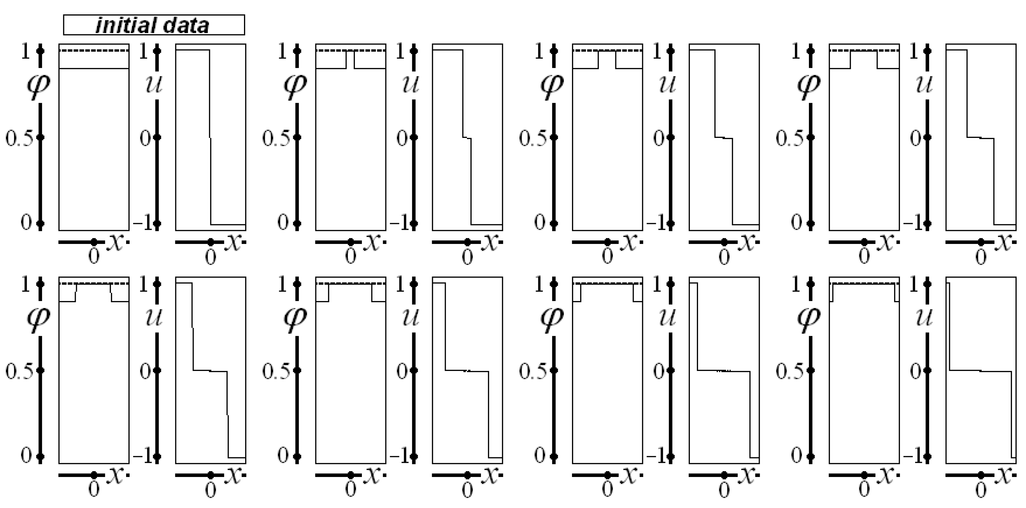
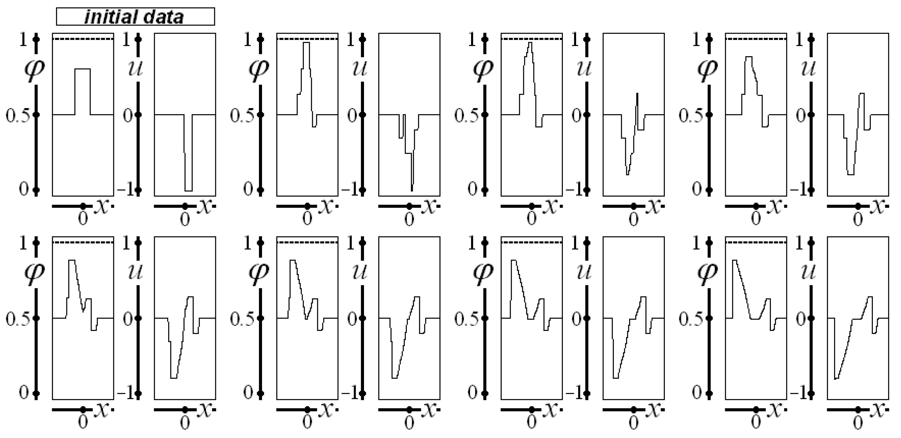
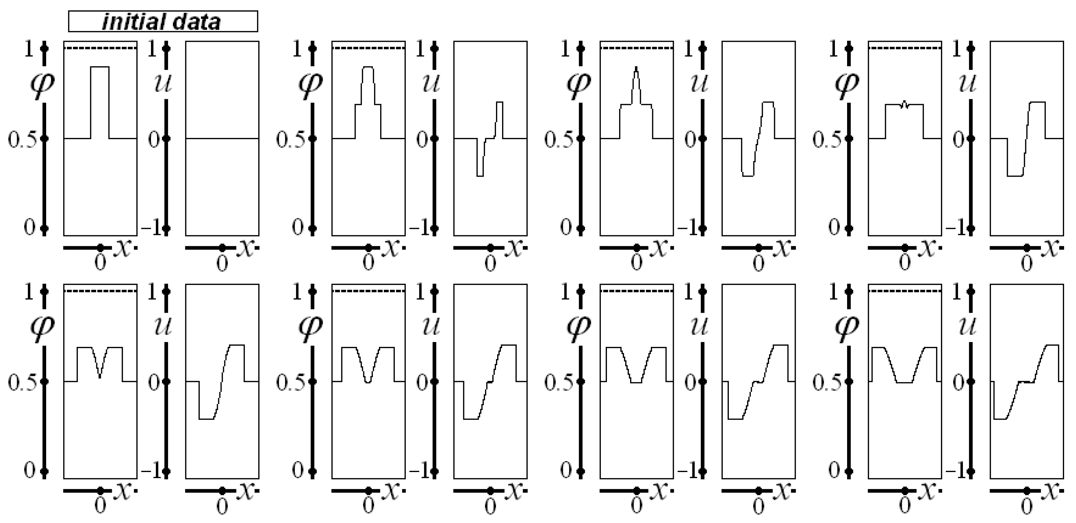
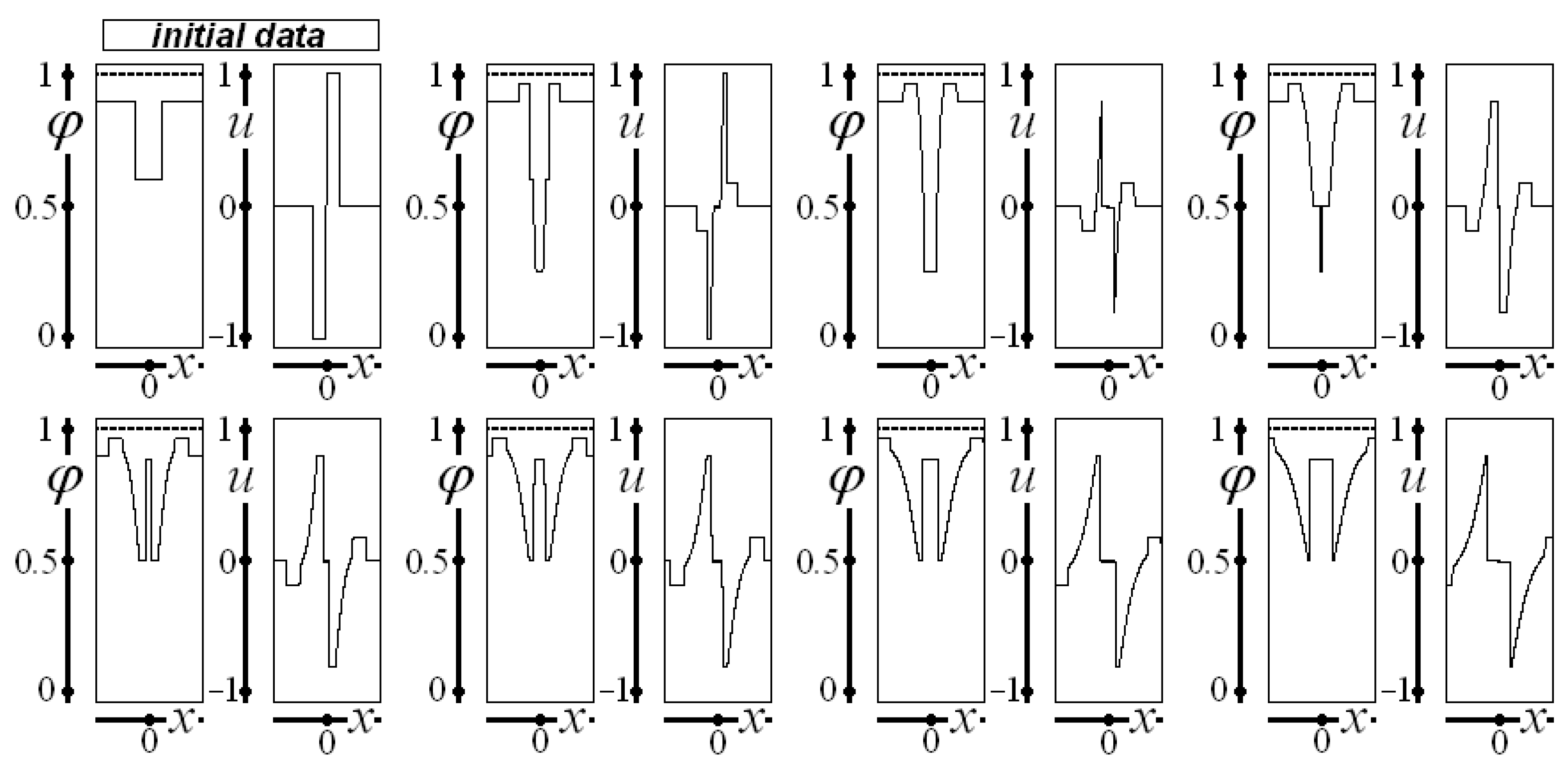
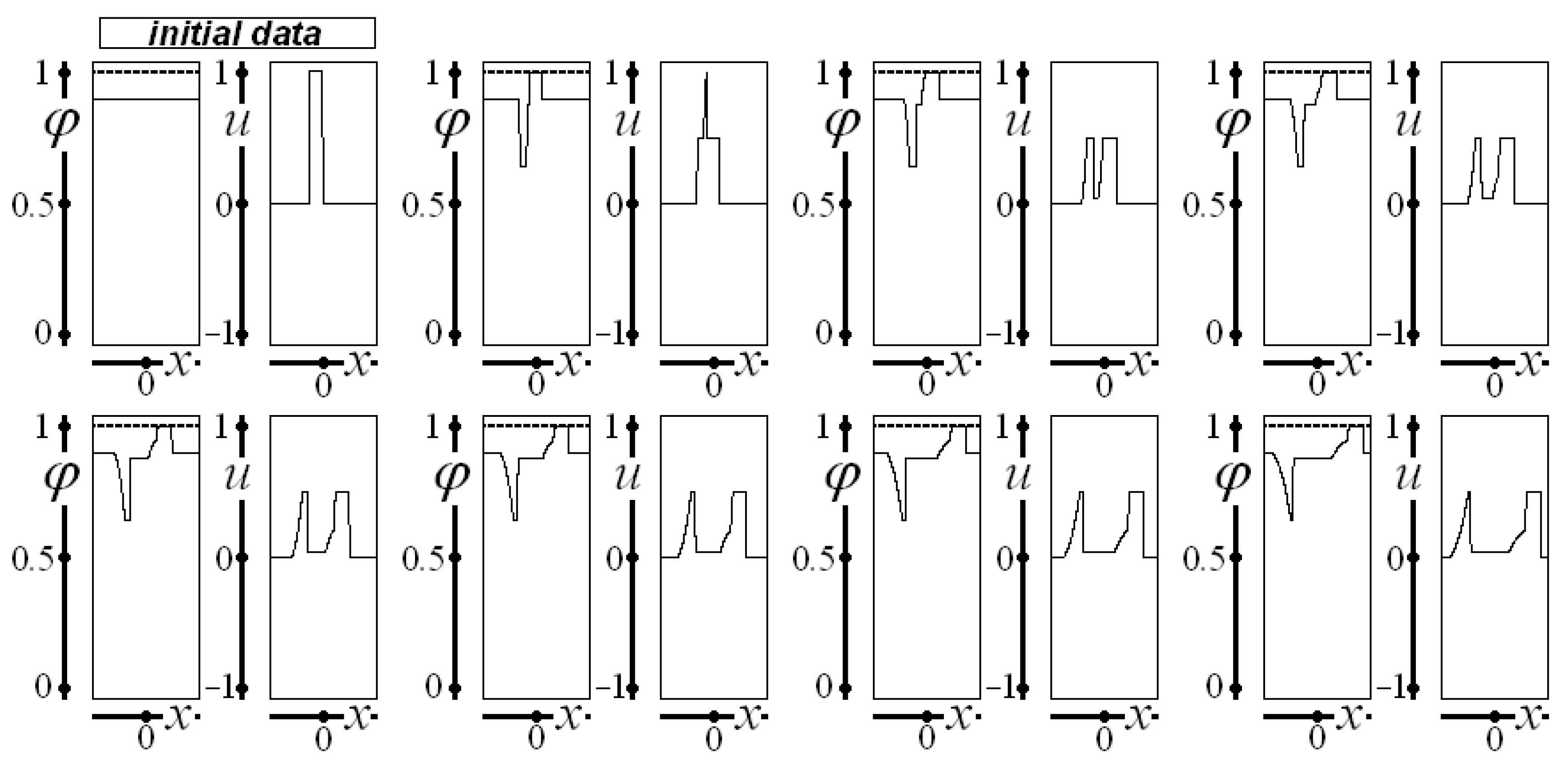
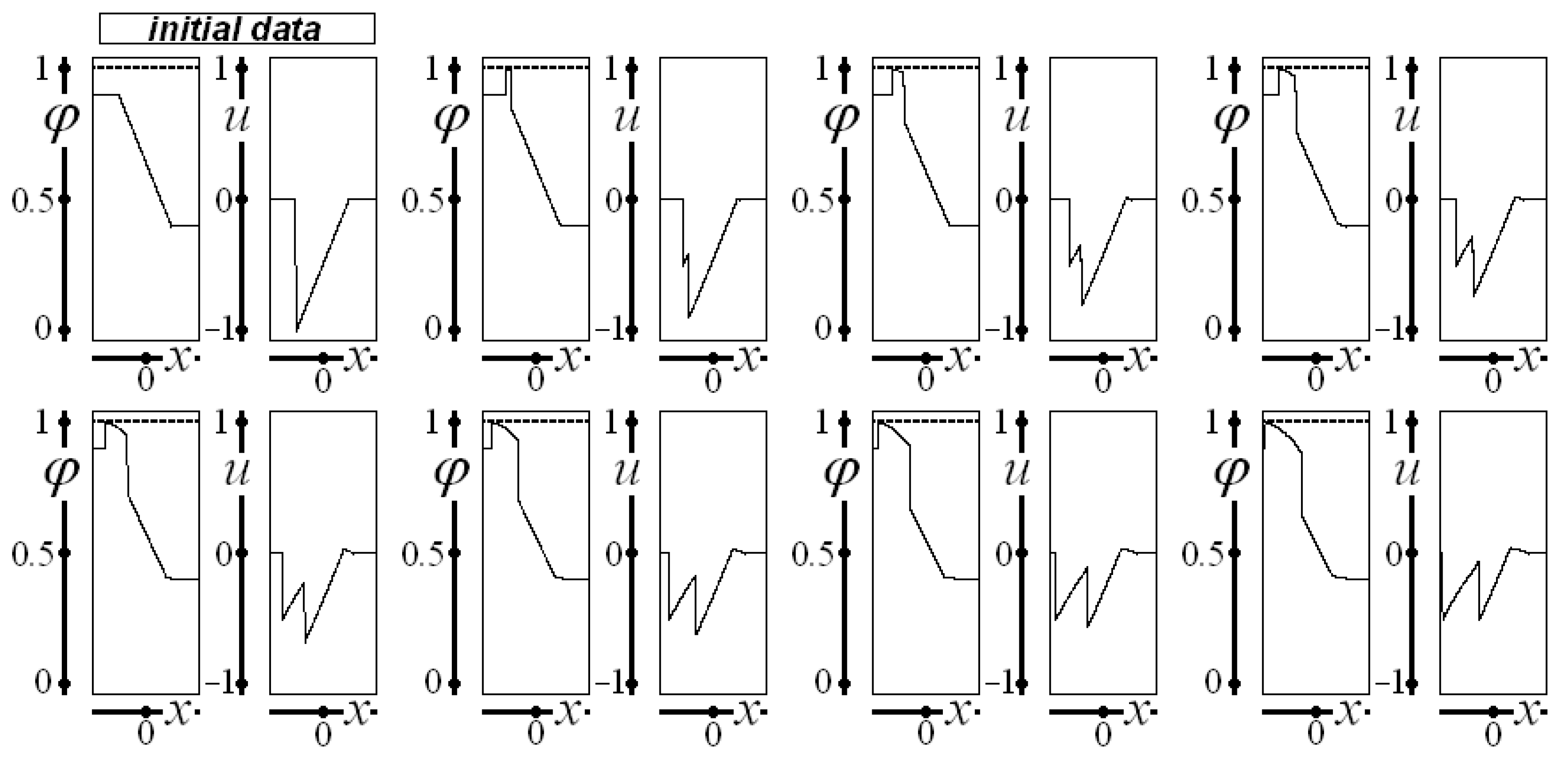
The construction of all of the following images follows the same structure: the first graph, on the upper left side, represents the initial data for saturation and velocity. The subsequent seven graphs represent the saturation and the velocity for $t=\gamma \Delta t$, $t=2\gamma \Delta t$, …, $t=6\gamma \Delta t$, and $t=7\gamma \Delta t$. All the figures represent the interval $x\in \left[-1,1\right]$.

The horizontal dashed line indicates the maximum allowable value for saturation ($\phi =1$).

Figure 1 depicts the evolution of saturation and velocity when initial data are given as $\phi =0.9 \mathrm{for} -\infty <x<\infty$,$u=+1.0 \mathrm{for} -\infty <x<0$, and $u=-1.0$ for $0\le x<\infty$, considering constant saturation, a step function with a very high constant saturation, and a step function ranging from the maximum considered velocity for negative $x$ values to the minimum considered velocity for positive $x$ values.

Note that saturation reaches a value near unity (saturated flow) in the first selected time instant. As expected, the width of the region with higher saturation increases as time evolves, so that at $t=7\gamma \Delta t$, almost the whole domain presents a saturation value near unity. The velocity value is zero in the same spatial regions, keeping the imposed initial values only at two minimal spatial regions. Note that the shocks are at the same spatial position for saturation and velocity.

Figure 2 presents the evolution of saturation and velocity considering $\phi =0.5 \mathrm{for} -\infty <x<-0.25\hspace{0.33em}\cup \hspace{0.33em}0.25<x<\infty$ and $\phi =0.8 \mathrm{for} -0.25\le x\le 0.25$, and $u=0.0 \mathrm{for} -\infty <x<0\hspace{0.33em}\cup \hspace{0.33em}0.25<x<\infty$ and $u=-1.0 \mathrm{for} 0\le x\le 0.25$ as initial data.

In Figure 2, saturation approaches unity only in a tiny spatial region in the two graphs after the initial data near the higher saturation imposed in the initial condition. The small region with higher saturation and the tiny region with low velocity provoke saturation and velocity variation along almost the whole domain, except for two narrow regions near the extremes of the interval $x\in \left[-1,1\right]$.

Figure 3 represents the behavior of saturation and velocity, with initial data $\phi =0.5 \mathrm{for} -\infty <x<-0.25\hspace{0.33em}\cup \hspace{0.33em}0.25<x<\infty$ and $\phi =0.8 \mathrm{for} -0.25\le x\le 0.25$ for saturation and $u=0.0 \mathrm{for} -\infty <x<\infty$ for velocity. A small region with higher saturation imposed at the center of the domain (with zero velocity) is sufficient to influence saturation and velocity throughout almost the whole spatial domain. However, saturation does not approach unity, as in the previous figures.

Figure 4 depicts saturation and velocity over time, considering $\phi =0.9 \mathrm{for} -\infty <x<-0.25\hspace{0.33em}\cup \hspace{0.33em}0.25<x<\infty$ and $\phi =0.6 \mathrm{for} -0.25\le x\le 0.25$ as initial data for saturation, while the initial velocity is given by $u=-1.0 \mathrm{for} -0.25\le x\le 0$ and $u=1.0 \mathrm{for} 0<x\le 0.25$. The lower saturation region and the tiny low- and high-velocity regions imposed as initial data influence saturation and velocity throughout the spatial domain; saturation barely approaches unity.

The initial data used to depict Figure 5 are constant saturation, with $\phi =0.9 \mathrm{for} -\infty <x<\infty$ and initial velocity $u=0.0 \mathrm{for} -\infty <x<-0.25\hspace{0.33em}\cup \hspace{0.33em}0<x<\infty$ and $u=1.0 \mathrm{for} -0.25\le x\le 0$, representing a tiny region with the maximum considered velocity. As in the previous figures, this tiny high-velocity region influences the behavior of saturation and velocity along the spatial domain. Also, as in Figure 1 and Figure 2, saturation approaches unity.

Figure 6 considers the following initial data for saturation: $\phi =0.9 \mathrm{for} -\infty <x<-0.25$, $\phi =0.4 \mathrm{for} 0.25<x<\infty$, and $\phi =0.65-x \mathrm{for} -0.25\le x\le 0.25$, and for velocity: $u=0.0 \mathrm{for} -\infty <x<-0.25\hspace{0.33em}\cup \hspace{0.33em}0.25<x<\infty$ and $u=2x-0.5 \mathrm{for} -0.25\le x\le 0.25$, characterizing linear decreasing saturation linked to constant values near the interval $x\in \left[-1,1\right]$ ends and constant zero velocities near the interval ends linked to a triangular shape with negative velocities. This shape abruptly reaches the minimum velocity and then increases as a linear function to zero. The initial data influence the whole spatial domain, and saturation approaches unity.

7. Final Remarks

The constitutive relation for the pressure proposed in this work allows a very small supersaturation of the porous matrix by the fluid. This supersaturation is controllable; any additional fluid inlet provokes a rapid and meaningful augmentation in pressure and speed propagation.

The model allows for preserving the hyperbolic nature of the problem and, employing Glimm’s method for the simulation, ensuring consistent physical results. The implementation of Glimm’s scheme depends on the random number sign, so a strategy using an average value of four different solutions obtained using the sequences of random numbers $\left\{+{\theta }_n\right\}$ and $\left\{-{\theta }_n\right\}$, provides more accurate results concerning shock wave and rarefaction wave positions. As the space interval decreases, the accuracy of the results improve.

This reliable tool adequately describes problems with the transition between saturated/unsaturated flow through porous media and vice versa and provides an accurate numerical solution via Glimm’s method.