Abstract
The partial singular value assignment problem stems from the development of observers for discrete-time descriptor systems and the resolution of ordinary differential equations. Conventional techniques mostly utilize singular value decomposition, which is unfeasible for large-scale systems owing to their relatively high complexity. By calculating the sparse basis of the null space associated with some orthogonal projections, the existence of the matrix in partial singular value assignment is proven and an algorithm is subsequently proposed for implementation, effectively avoiding the full singular value decomposition of the existing methods. Numerical examples exhibit the efficiency of the presented method.
Keywords:
partial singular value assignment; large-scale system; sparse basis; orthogonal projection MSC:
65F99
1. Introduction
Partial singular value assignment (PSVA) is a powerful technique with application in a variety of fields, including control theory, optimization problems, signal processing and many more [1,2,3,4,5,6,7,8,9,10]. PSVA focuses on selectively modifying the singular values of a matrix while keeping others unchanged. This technique enables engineers, researchers, and practitioners to address various problems in a nuanced and efficient manner. Notably, PSVA plays a pivotal role in minimizing errors when designing observers for the following discrete-time descriptor systems
where the coefficient matrices E, , and , and are the system errors; , and are the state vector, input vector and output vector, respectively. This system, initially introduced by Luenberger in 1977 [11], has been extensively explored, particularly in cases involving the singular matrix E. Contemporary research has yielded a wealth of theoretical insights from control theorists and numerical analysts, covering the continuous-time descriptor systems. These investigations encompass a wide array of subjects, including controllability, observability [12,13], pole assignment [14,15], eigenstructure assignment [16], Kronecker’s canonical form [17], solution algorithms [18] and the inequality method [19]. It is worth noting that many of the findings from these studies are applicable to discrete-time systems as well.
In the context of the discrete-time descriptor system, the observer can be described as follows
where H, . The resulting error vector,
satisfies the equality
A key objective in PSVA is to find a matrix H such that the smallest singular values (which might be zeros) of are sufficiently large, or, equivalently, the norm of is sufficiently small; it then greatly reduces the impact of unmodeled error terms [20,21]. For further insights into the error reduction achieved by PSVA in other optimal state-space controller designs, such as and systems, please refer to [22,23] for detailed discussions.
PSVA has another important application in numerical methods solving ordinary differential equations (ODEs) [24]. It is widely recognized that Euler’s method plays a crucial role in the context of ODEs. Despite its rapidly increasing error as calculations progress, Euler’s method stands out as one of the few options in generating initial values needed for higher-order methods. When we apply the explicit Euler method to a differential equation with initial values, the resulting numerical solution tends to underestimate the true solution. Conversely, when we employ the implicit Euler method, the numerical method tends to overestimate the true solution. This suggests that a combination of these two methods could lead to better results. However, straightforward averaging has its limitations. An intriguing alternative is to consider “randomly switching” between the two methods. If we average all possible outcomes generated by the “random switching”, the resulting method can be approximately tens or even hundreds of times more accurate than either the explicit or implicit Euler method. For example, consider a numerically linear method to solve the ODE given by
with being a constant; the numerical solution can be achieved by closing a feedback loop, following the principles of linear control theory [24].
In our discussion, we will leverage this control to modify the method so that singular values can be assigned. To illustrate this, we consider two linear methods
and
of solving the differential Equation (1), where b, g, c and h are vectors of compatible dimensions with the systems above. The matrices A and F, both belonging to , possess properties determined by the chosen numerical method. However, they share the common attribute of having 1 as an eigenvalue with a multiplicity of 1. If there are other eigenvalues located on the unit circle, they also have a multiplicity of 1, while all remaining eigenvalues lie within the unit circle.
Similar to the improvements achieved with the Euler methods, a natural enhancement of the linear method can be obtained by randomly switching between these two linear methods. In practice, the feedback loop in control theory yields the following results:
and
Let be a random variable with values in . The “random switching” iteration
depends heavily on the product
It has been shown in [25] that the “random switching” iteration converges if and only if the 2-norm of is less than 1. Since the 2-norm of associates with the largest singular value, it raises the question of when the singular values of a linear system can be assigned through the state feedback.
The above applications indicate that the PSVA problem involves assigning several desired singular values and determining how the remaining singular values behave. In mathematics, PSVA can be expressed explicitly as follows.
- PSVA: Given matrices A, B and the desired (non-zero) singular values , find a matrix F such thathas the p desired singular values.
This problem was initially addressed in [20] for small and medium-scale systems. Typically, one needs a full QR decomposition of matrix B, i.e.,
and a full singular value decomposition (SVD) to construct the matrix F. If all singular values need to be reassigned, the interlacing theory on singular values of and an SVD of the orthogonal projection of A onto the null space of B are required for the formation of F [26]. However, for large-scale systems, methods related to the full SVD of a large matrix are not feasible due to the computational complexity of and memory limitations. Similar issues were encountered in pole assignment [14,15,27,28]. Readers can find details in [29,30,31,32] and their references.
In this paper, we introduce an efficient algorithm to conduct PSVA on large-scale systems. The primary contributions and advantages of our algorithm are listed below.
- The core innovation of our devised approach is rooted in the construction of a sparse basis within the null space of the orthogonal projection of matrix A. This strategy offers a notable advantage by obviating the necessity for the full SVD of a large-scale matrix.
- Our algorithm brings to the forefront the possibility of computational savings, especially when dealing with matrices of significant scale and sparse structure (i.e., the number of non-zeros in each column of the matrix is bounded by a constant much smaller than n). Then, the proposed algorithm strives to assign the desired singular values with exceptional computational efficiency, hopefully scaling with the computational complexity of floating-point operations.
- To validate the practical utility of our proposed algorithm, we conduct a series of numerical experiments. These experiments not only confirm the feasibility of our approach but also demonstrate its effectiveness in real-world scenarios.
Throughout this paper, we denote the i-th singular value, 2-norm and the condition number of by , (the maximal singular value) and (the ratio of the maximal and the minimal singular value), respectively. The determinant of the matrix A is represented by . The equivalence of two pairs of matrices is defined as follows.
Definition 1
([33]). Two pairs of matrices and are equivalent if there are orthogonal matrices U and V, a matrix E and a nonsingular matrix R with compatible sizes such that
The equivalence of matrix pairs is attractive as it preserves the same assignability of singular values. Thus, one can use the simplest representation to describe a class of equivalent pairs and study the existence of PSVA.
2. PSVA for Single Singular Value
We first delve into the single PSVA. This problem can be simplified to the following.
- Single PSVA: Given a matrix , a vector and the desired (non-zero) singular values , find a vector such thatinclues the desired singular value .
To solve the single PSVA, we initiate the process by ensuring that the smallest singular value of a matrix associated with A is in proximity to zero, or even equal to zero. Once this condition is met, we can proceed with constructing the orthogonal projection of matrix A onto the null space of vector b by using
which effectively enforces a minimal singular value of zero. In fact, by performing the QR decomposition of b by
where and , we have the smallest singular value of
forced to be zero. Let the SVD of D be given by
where and are orthogonal matrices with ; , , , is a diagonal matrix with its non-zero diagonal elements being the singular values of D. We can demonstrate the existence of the single PSVA through the following theorem.
Theorem 1.
For a given singular value , there exists a vector such that the singular values of are .
Proof.
We can then define vectors with and . As a result, we have
with
and for . The assignment of the singular value in is now reduced to the assignment in according to Definition 1.
Now, we consider the characteristic polynomial of the matrix . It follows
By letting
with , we see that there are multiple solutions to Equation (5). One simple choice is to take and . By setting , we have the desired vector of to complete the PSVA for a single singular value. □
Remark 1.
Although there are multiple solutions to Equation (5), e.g., the vector z could be also taken as
the choice of in Theorem 1 is the most valid as it ensures that the other () is also a root of .
The above theorem provides the motivation for constructing the vector f for the single PSVA. In fact, by equating the two sides of the SVD of D in (4), it follows that
By taking and as and , respectively, then, for a singular value of to be assigned, we have
and the vector
completes the single PSVA. Algorithm 1 outlines the concrete steps involved in the single PSVA.
| Algorithm 1 PSVA for the Single Singular Value |
Input: A large-scale sparse matrix , and the desired singular value . Output: A vector such that the minimal singular value of is . 1. Compute ; 2. Compute the economic QR decomposition of b, i.e., ; 3. Compute the null space of the matrix ; 4. Form the vector such that the smallest singular value of is . |
Remark 2.
(1) The QR decomposition of b has a complexity of when the Householder transformation is used [34].
(2) The vector in the null space of
should be as sparse as possible. Two methods have been tested in our experiments. One involves computing the complement of using the QR decomposition, while the other involves computing the LU factorization. If the elements in each column of A are sparse, with an upper bound of a (which is much less than n), then the computational complexity may hopefully be .
3. PSVA for p Singular Values
The single PSVA can be readily generalized to the p singular value assignment with .
- p-PSVA: Given a large-scale sparse matrix with p smallest singular values being close to (or equal to) zero, and a matrix , find a matrix such thatits p smallest singular values are the given .
Let us construct the matrix
which is the orthogonal projection of A on the null space of B. By using the QR decomposition of B
with , the matrix
will have p zero singular values. Let the SVD of D be
with the diagonal matrix having the diagonal elements . The following theorem provides the existence of the PSVA.
Theorem 2.
For singular values to be assigned, there exists a matrix such that the singular values of are .
Proof.
Set
for . According to Definition 1, the form of must be determined such that the singular values of are those of . Firstly, consider . By setting with and other elements being zeros, Theorem 1 indicates that there exists a vector such that the non-zero singular values of are . By using induction and Theorem 1 continuously, it can be shown that there is a matrix such that the singular values of are . □
We can further elaborate on the form of F in terms of Theorem 2. In fact, let the orthogonal matrices U and V in (4) be given as
with , , respectively. Then, by setting and , we have
where represents a diagonal matrix, with its diagonal elements containing the desired non-zero singular values . Furthermore, the matrix F can be expressed as
The steps involved in the PSVA for p singular values are outlined in Algorithm 2.
A crucial aspect of Algorithm 2 is to minimize the sparsity of the computation for the null sparse basis of matrix D. While the heuristic method suggested in [20] is an option, empirical testing has revealed that QR decomposition or LU factorization in MATLAB can produce adequately sparse vectors, particularly when the matrix A possesses a significant degree of sparsity.
Remark 3.
As indicated by Remark 2, the computational complexity of Algorithm 2 is advantageous, with a time complexity of when the matrix A exhibits a degree of sparsity (characterized by relatively small values of a and p in comparison to the matrix size n). In this case, Algorithm 2 offers a substantial advantage over methods relying on the the full SVD, which typically entail a much higher time complexity of . This stark contrast positions Algorithm 2 as a clear choice for the handling of large-scale systems, where the efficiency and computational speed are obviously superior. Moreover, when the matrix A reaches a considerable order (scaling up to the thousands), methods that rely on the full SVD approach tend to become prohibitively time-consuming, particularly when executed on standard personal computers. This temporal limitation restricts their applicability and practicality. This also the reason for exclusively showing the performance of our algorithm through numerical experiments on large-scale problems.
| Algorithm 2 PSVA for p Singular Values |
Input: A large-scale sparse matrix , and the desired singular values . Output: A matrix such that p smallest singular values of are . 1. Compute the economic QR decomposition of B, i.e., with and
2. Compute the null space of with . 3. Compute by Algorithm 1 with the available A, and . 4. For End. 5. Form the matrix such that the smallest p singular values of are . |
Another consideration in PSVA is to keep the condition number of the assigned matrix relatively low. This can be achieved through optimization methods based on heuristic rules [29,30]. For instance, Shields [21] employed the optimization of some matrix function over a set of assigned matrices with a fixed condition number. However, this approach becomes unfeasible for large-scale problems due to the full SVD of a large matrix. On the other hand, if the singular values assigned are well separated from those in , the following theorem shows that the condition number of will be no worse than that of .
Theorem 3
([21]). For any matrix
with being nonsingular and
the matrix F in the PSVA satisfies
Furthermore, there exists a non-unique matrix F to make the equality hold.
Remark 4.
From Theorem 3, it follows that will have a poor condition number if the gap between the maximal and the minimal singular values of is large. Conversely, if suitable singular values and a proper F are chosen to implement the PSVA, the obtained condition number of may be as close to that of as possible. This fact can be used to assess the effectiveness of Algorithm 2 in the next section.
4. Numerical Examples
In this section, we examine the efficacy of Algorithm 2 in addressing large-scale PSVA problems. The algorithm was coded by MATLAB 2014 and all examples were executed on a desktop equipped with an Intel i5 3.4 GHz processor and 16 GB RAM. We denote the authentically assigned singular value by and the computed singular value by . The relative error is computed as
when the matrix F is at hand.
We opted not to carry out a direct comparison between Algorithm 2 and the methods based on full SVD. The rationale behind this choice is grounded in the fact, as stated in Remark 3, these conventional approaches can become excessively time-consuming, particularly when executed on typical personal desktop setups.
Example 1.
For , we set and , where and are random numbers drawn from a uniformed distribution over the interval (generated by the MATLAB command “rand(n,1)”). We define the matrices
and
The singular values to be assigned are .
Algorithm 2 was utilized to carry out the PSVA, and 50 random experiments were conducted for n = 10,000. The resulting errors are depicted in Figure 1, with the vertical axis representing the error level and the horizontal axis reflecting the number of experiments. The assigned singular values are , corresponding to . It is evident from Figure 1 that all errors are within a range of . Furthermore, it is noteworthy that among 50 experiments, the errors of the assigned singular values (represented by the star line) and (represented by the diamond line) fluctuate more dramatically compared to the other errors, while the errors of (represented by the cross line) fluctuate the least.
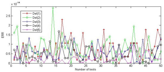
Figure 1.
Errors of 50 random tests in Example 1.
In Figure 2, we also list the computed CPU time and condition numbers of matrices D (CondS) and (CondPSVA), with all data on the vertical axis being recorded in to minimize the gaps between the various lines. It can be seen that the CPU time of all tests is approximately 0.7 s, and the range of CondPSVA lies between 48.1 and 51.5, compared to that of CondS, which lies between 8.81 and 13.43. This highlights the efficiency of Algorithm 2 in carrying out PSVA. It is worth mentioning that the condition number of is closely linked to the assigned singular values. In our experiments, we observed that CondPSVA approached CondS more closely when the minimal singular values to be assigned were larger.
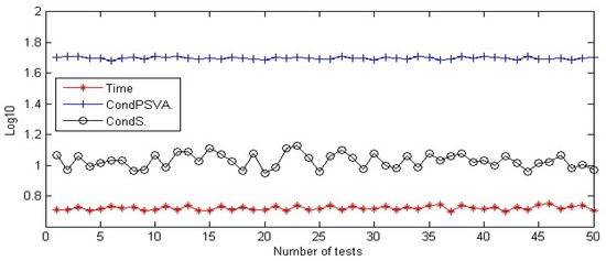
Figure 2.
Condition number and time of 50 random tests in Example 1.
Example 2.
This example is taken from a random perturbation of the PDE problem. We set n = 10,000 and define matrices A and B as
where in A are random numbers from the normal distribution, and the numbers in the middle columns of the matrix are 4999, 5000 and 5001. As in Example 1, we conduct 50 random experiments and assign singular values .
Figure 3 presents the results from 50 tests, with a specific focus on the obtained errors. Within this figure, the vector represents the assigned singular values corresponding to . A notable observation from the data displayed in Figure 3 is that all of the errors fall well below the threshold of , suggesting a high degree of accuracy in the assignment of singular values. Furthermore, the range of fluctuation among these errors is relatively small. In other words, the variations between the assigned singular values and the desired values are quite minor, reinforcing the precision and consistency of the assignments.
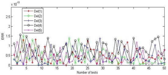
Figure 3.
Error in 50 random tests in Example 2.
We also present the consumed CPU time in Figure 4, which shows that the range varies from 0.40 to 0.46 s. The obtained CondS and CondPSVA of 50 random experiments fall within the interval [4.47, 9.11] and [366.53, 435.61], respectively (with the exception of the value 160.74 in the 35th experiment). Analogously, the value of CondPSVA can be reduced further by assigning relatively larger singular values in . In fact, if the assigned singular values are increased to 160, 162, 164, 166 and 168, the condition number of in 50 random experiments will fall within the interval [8.05, 12.30].
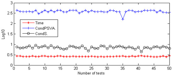
Figure 4.
Condition number and time of 50 random tests in Example 2.
Example 3.
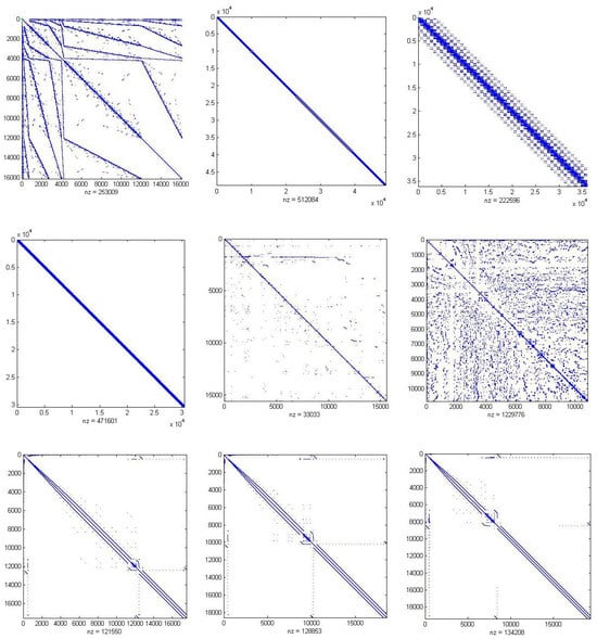
In this example, we seek to affirm the robustness and efficiency of Algorithm 2 by subjecting it to real-world testing. The examination involves the application of this algorithm to nine large-scale sparse matrices, which have been drawn from practical applications. These specific matrices are conveniently available in the SuiteSparse Matrix Collection, which was previously known as the University of Florida Sparse Matrix Collection, accessed via the following link: https://sparse.tamu.edu/, accessed on 10 September 2023.
The matrices under scrutiny bear the following names: ‘dubcova1’, ‘gridgena’, ‘onetone2’, ‘wathen100’, ’poli_large’, ‘msc10848’, ‘bodyy4’, ‘bodyy5’ and ‘bodyy6’. Each of these matrices varies in size, catering to the demands of diverse applications. The dimensions of these matrices are as follows: 16,129 × 16,129, 48,962 × 48,962, 36,057 × 36,057, 30,401 × 30,401, 15,575 × 15,575, 10,848 × 10,848, 17,546 × 17,546, 18,589 × 18,589 and 19,366 × 19,366. Their sparse structures are plotted in Figure 5, where ‘nz’ indicates the non-zero elements.

Figure 5.
Sparse structures of nine matrices in Example 3.
In our experiments, the matrix
remains invariant for all different problems, but the two assigned singular values vary for each matrix.
We ran Algorithm 2 in dealing with the nine large-scale matrices and the obtained results are exhibited in Table 1. The CPU column in the table provides information regarding the elapsed time, measured in seconds, required to perform the PSVA. The DesSV and AsiSV columns, respectively, denote the two sets of singular values, one representing the desired values (DesSV) and the other representing the values that were actually assigned (AsiSV). These columns allow us to assess how closely the assigned singular values align with the desired values. They serve as a crucial indicator of the accuracy and precision of the PSVA process. The next column, labeled RelErr, offers insights into the relative errors encountered during the PSVA computation. A smaller relative error indicates the more accurate assignment of singular values. The final two columns, CondS and CondPSVA, provide information about the condition numbers of two distinct entities. CondS represents the condition number of , while CondPSVA represents the condition number of the matrix . These condition numbers help to assess the numerical stability and quality of the PSVA solution. Smaller condition numbers are indicative of more favorable and robust solutions.

Table 1.
Assigned results for nine large-scale matrices in Example 3.
It can be seen that Algorithm 2 is efficient in assigning the required two singular values in a relatively short CPU time for all matrices. The RelErr column indicates that the relative error is very small, except for two matrices, ‘gridgena’ and ‘msc10848’, with respective levels and . The CondS column lists the condition numbers of for different matrices, where a larger order means a wider gap between the maximal and the minimal singular values. The CondPSVA column records the condition number of after the assignment, showing a relatively modest increase in the condition number from CondS. This also reflects that Algorithm 2 is efficient in implementing PSVA, as stated in Remark 4, and provides valuable insights into the algorithm’s capacity to handle complex, large-scale, real-world systems.
5. Conclusions
In the context of large-scale discrete-time systems, a novel algorithm has been introduced to facilitate partial singular value assignment (PSVA), particularly when the matrices A and B exhibit a significant degree of sparsity. This method leverages the capabilities of a sparse solver and incorporates the orthogonal projection of matrix A onto the null space of matrix B as a fundamental component. Crucially, we have established the existence of a matrix F that plays a pivotal role in both single and multiple PSVA problems. This implies that it can be applied effectively to address a range of singular value assignment scenarios, offering flexibility and versatility in practical applications.
The proposed approach is validated through a series of numerical experiments. The derived results affirm the algorithm’s efficacy in achieving the partial assignment of desired singular values, thereby underscoring its real-world applicability for large-scale discrete-time systems. For future research, we will explore the possibility to tackle more complex and practical systems in various fields, from control theory to areas of signal processing.
Author Contributions
Conceptualization, B.Y.; methodology, B.Y.; software, Y.H.; validation, Y.H.; and formal analysis, Q.T. All authors have read and agreed to the final version of this manuscript.
Funding
This work was supported partly by the NSF of Hunan Province (2021JJ50032, 2023JJ50164, 2023JJ50165), the NSF of China (12305016), Degree and Postgraduate Education Reform Project of Hunan University of Technology and Hunan Province (JG2315, 2023JGYB210).
Acknowledgments
We are grateful to the anonymous referees for their useful comments and suggestions, which significantly enhanced the quality the original paper.
Conflicts of Interest
The authors declare no conflict of interest.
References
- Bangle, H.E. Feature extraction of cable partial discharge signal based on DT_CWT_Hankel_SVD. In Proceedings of the 2019 6th International Conference on Information Science and Control Engineering (ICISCE), Shanghai, China, 20–22 December 2019; pp. 1063–1067. [Google Scholar]
- Cooke, S.A.; Minei, A.J. The pure rotational spectrum of 1, 1, 2, 2, 3-pentafluorocyclobutane and applications of singular value decomposition signal processing. J. Mol. Spectrosc. 2014, 306, 37–41. [Google Scholar] [CrossRef]
- Datta, B.N. Linear and numerical linear algebra in control theory: Some research problems. Linear Algebra Its Appl. 1994, 197, 755–790. [Google Scholar] [CrossRef]
- Hou, Z.; Jin, S. Model Free Adaptive Control: Theory and Applications; CRC Press: Boca Raton, FL, USA, 2013. [Google Scholar]
- Sontag, E.D. Mathematical Control Theory: Deterministic Finite Dimensional Systems; Springer Science & Business Media: New York, NY, USA, 2013; Volume 6. [Google Scholar]
- Sogaard-Andersen, P.; Trostmann, E.; Conrad, F. A singular value sensitivity approach to robust eigenstructure assignment. In Proceedings of the 1986 25th IEEE Conference on Decision and Control, Athens, Greece, 10–12 December 1986; pp. 121–126. [Google Scholar]
- Van Dooren, P. Some numerical challenges in control theory. In Linear Algebra for Control Theory; Springer: New York, NY, USA, 1994; pp. 177–189. [Google Scholar]
- Weinmann, A. Uncertain Models and Robust Control; Springer Science & Business Media: Vienna, Austria, 2012. [Google Scholar]
- Zimmerman, D.C.; Kaouk, M. Eigenstructure assignment approach for structural damage detection. AIAA J. 1992, 30, 1848–1855. [Google Scholar] [CrossRef]
- Saraf, P.; Balasubramaniam, K.; Hadidi, R.; Makram, E. Partial right eigenstructure assignment based design of robust damping controller. In Proceedings of the 2016 IEEE Power and Energy Society General Meeting (PESGM), Boston, MA, USA, 17–21 July 2016; pp. 1–5. [Google Scholar]
- Luenberger, D. Dynamic equations in descriptor form. IEEE Trans. Autom. Control 1977, 22, 312–321. [Google Scholar] [CrossRef]
- Ishihara, J.Y.; Terra, M.H. Impulse controllability and observability of rectangular descriptor systems. IEEE Trans. Autom. Control 2001, 46, 991–994. [Google Scholar] [CrossRef]
- Feng, Y.; Yagoubi, M. Robust Control of Linear Descriptor Systems; Springer: Singapore, 2017. [Google Scholar]
- Chu, E.K. A pole-assignment algorithm for linear state feedback. Syst. Control. Lett. 1986, 7, 289–299. [Google Scholar] [CrossRef]
- Chu, E.K. A pole-assignment problem for 2-dimensional linear discrete systems. Int. J. Control 1986, 43, 957–964. [Google Scholar] [CrossRef]
- Duan, G.R. Eigenstructure assignment in descriptor systems via output feedback: A new complete parametric approach. Int. J. Control 1999, 72, 345–364. [Google Scholar] [CrossRef]
- Kumar, A.; Kumar, A.; Pait, I.M.; Gupta, M.K. Analysis of impulsive modes in Kronecker Canonical form for rectangular descriptor systems. In Proceedings of the IEEE 8th Indian Control Conference (ICC), Chennai, India, 14–16 December 2022; pp. 349–354. [Google Scholar]
- Shahzad, A.; Jones, B.L.; Kerrigan, E.C.; Constantinides, G.A. An efficient algorithm for the solution of a coupled Sylvester equation appearing in descriptor systems. Automatica 2011, 47, 244–248. [Google Scholar] [CrossRef]
- Masubuchi, I.; Kamitane, Y.; Ohara, A.; Suda, N. H∞ control for descriptor systems: A matrix inequalities approach. Automatica 1997, 33, 669–673. [Google Scholar] [CrossRef]
- Pearson, D.W.; Chapman, M.J.; Shields, D.N. Partial singular-value assignment in the design of robust observer for discrete-time descriptor systems. IMA J. Math. Control Inform. 1988, 5, 203–213. [Google Scholar] [CrossRef]
- Shields, D.N. Singular-value assignment in the design of observers for discrete-time systems. IMA J. Math. Control Inform. 1991, 8, 151–164. [Google Scholar] [CrossRef]
- Hague, T.N. An Application of Robust H2/H∞ Control Synthesis to Launch Vehicle Ascent. Ph.D. Thesis, Department of Aeronautics and Astronautics, Massachusetts Institute of Technology, Cambridge, MA, USA, 2000. [Google Scholar]
- Sun, X.D.; Clarke, T. Application of hybrid μH∞ control to modern helicopters. In Proceedings of the International Conference on Control (Control’94 IET), Coventry, UK, 21–24 March 1994; Volume 2, pp. 1532–1537. [Google Scholar]
- Holder, D.; Luo, S.; Martin, C. The control of error in numerical methods, in modeling, estimation and control. In Lecture Notes in Control and Information Sciences; Springer: Berlin/Heidelberg, Germany, 2007; pp. 183–192. [Google Scholar]
- Elsner, L.; Friedland, S. Norm conditions for the convergence of infinite products. Linear Algebra Appl. 1997, 250, 133–142. [Google Scholar] [CrossRef][Green Version]
- Martin, C.F.; Wang, X.A. Singular value assignment. SIAM J. Control Optim. 2009, 48, 2388–2406. [Google Scholar] [CrossRef]
- Kautsky, J.; Nichols, N.K.; Van Dooren, P. Robust pole assignment in linear state feedback. Int. J. Control. 1985, 41, 1129–1155. [Google Scholar] [CrossRef]
- Nichols, N.K. Robustness in partial pole placement. IEEE Trans. Auto. Control 1987, 32, 728–732. [Google Scholar] [CrossRef]
- Chu, E.K. Optimisation and pole assignment in control system design. Int. J. Appl. Math. Comput. Sci. 2001, 11, 1035–1053. [Google Scholar]
- Datta, S.; Chakraborty, D.; Chaudhuri, B. Partial pole placement with controller optimization. IEEE Tans. Auto. Control 2012, 57, 1051–1056. [Google Scholar] [CrossRef]
- Datta, S.; Chaudhuri, B.; Chakraborty, D. Partial pole placement with minimum norm controller. In Proceedings of the 49th IEEE Conference on Decision and Control, Atlanta, GA, USA, 15–17 December 2010; pp. 5001–5006. [Google Scholar]
- Saad, Y. Projection and deflation methods for partial pole assignment in linear state feedback. IEEE Trans. Automat. Control 1988, 33, 290–297. [Google Scholar] [CrossRef]
- Horn, R.A.; Johnson, C.R. Matrix Analysis; Cambridge University Press: Cambridge, UK, 1985. [Google Scholar]
- Golub, G.H.; Van Loan, C.F. Matrix Computations; Johns Hopkins University Press: Baltimore, MD, USA, 1996. [Google Scholar]
Disclaimer/Publisher’s Note: The statements, opinions and data contained in all publications are solely those of the individual author(s) and contributor(s) and not of MDPI and/or the editor(s). MDPI and/or the editor(s) disclaim responsibility for any injury to people or property resulting from any ideas, methods, instructions or products referred to in the content. |
© 2023 by the authors. Licensee MDPI, Basel, Switzerland. This article is an open access article distributed under the terms and conditions of the Creative Commons Attribution (CC BY) license (https://creativecommons.org/licenses/by/4.0/).