Abstract
The aim of this paper is to present and study nonlinear bivariate quadratic spline quasi-interpolants on uniform criss-cross triangulations for the approximation of piecewise smooth functions. Indeed, by using classical spline quasi-interpolants, the Gibbs phenomenon appears when approximating near discontinuities. Here, we use weighted essentially non-oscillatory techniques to modify classical quasi-interpolants in order to avoid oscillations near discontinuities and maintain high-order accuracy in smooth regions. We study the convergence properties of the proposed quasi-interpolants and we provide some numerical and graphical tests confirming the theoretical results.
MSC:
65D05; 65D07; 65D15; 65D17; 41A15; 41A81
1. Introduction
In the context of function and data approximation (an important problem in many mathematical and scientific applications), quasi-interpolation is well known to be a powerful and useful tool (as evidenced in [1] and references [2,3,4,5] for applications of spline quasi-interpolation). In particular, a nice property of quasi-interpolation, if compared to interpolation, is that it does not require the solution of any system of equations. This property is particularly attractive in the two-dimensional case, where the data volume can be huge, in practice. Moreover, interpolation requires that the approximant exactly matches the data at certain points; this requirement could be a problem if we are dealing with noisy data.
If the function to be approximated is smooth, a spline quasi-interpolant (QI) is able to well reconstruct it, but if the function has jump discontinuities, the approximating spline presents oscillations of magnitude proportional to the jump. Therefore, the aim of this paper is to apply weighted essentially non-oscillatory (WENO) techniques in the definition of the spline QI to avoid such oscillations. Using such a nonlinear modification, we are able to avoid the Gibbs phenomenon near discontinuities and, at the same time, maintain high-order accuracy in smooth regions. This problem has been faced in the univariate case in [6], applying the technique to quadratic and cubic spline QIs (as evidenced in reference [7]). Here, we move toward the bivariate setting. In particular, we consider quadratic spline QIs on uniform criss-cross triangulations of a rectangular domain, which can be expressed by means of the scaled/translates of the Zwart–Powell quadratic box spline (ZP element) (see, e.g., [8] (Chapter 1) and [9] (Chapter 2)). We should note that quadratic spline spaces on criss-cross triangulations have been widely studied in the literature (see, e.g., [10,11,12,13,14,15,16,17] and references therein, and more recent papers, [18,19,20]), with reference to the dimension, local basis, approximation power, etc.; they have been used in many applications. We are aware that the use of non-uniform knot partitions and multiple knots in the spline space definition can sometimes mimic function discontinuities of the approximating function (see, e.g., [21]), but such a possibility requires knowledge of discontinuity locations. In contrast, using the technique presented in this paper, we are able to deal with discontinuities without knowing where they are; it can also be applied to general cases. Moreover, the use of box splines on uniform partitions represents an advantage—from a computational point of view—with respect to the use of non-uniform ones.
The paper is organized as follows. In Section 2, we define the spline space, and recall definitions and properties of spline quasi-interpolant operators. Then, in Section 3, we recall the WENO techniques. In Section 4, we apply the techniques of the previous section for constructing nonlinear spline quasi-interpolants and study their properties. In Section 5, we provide numerical and graphical tests, confirming the theoretical results of Section 4. Finally, in Section 6, we present some conclusions.
2. The Spline Space
Let be a rectangular domain divided into equal squares, each of them being subdivided into four triangles by its diagonals. We denote by the space of quadratic splines on the triangulation of obtained in this way. This space is generated by the spline functions , where , obtained by the dilation/translation of the Zwart–Powell quadratic box spline (ZP element) ([8] (Chapter 1) and [22] (Chapter 3)).
The ZP element is the bivariate quadratic box spline supported on the octagon with the center at the origin and vertices at , , , , , , , . It is strictly positive inside its support, which is partitioned into 28 triangular cells. On every cell, the ZP element is a polynomial of total degree 2, and in [11], the polynomials are given. The ZP element can also be expressed in BB form, i.e., specifying the Bernstein–Bézier (abbr. BB) coefficients on every triangular cell [23] (Chapter 6). We denote by the support of the dilated/translated box spline , and its center by .
In the space , we consider linear quasi-interpolants (QIs) with the following form:
where is a set of continuous linear forms, called coefficient functionals. They can be of different types, chosen according to the provided information about the function f to be approximated. Usually, they are point, derivative, or integral linear functionals. In the first case, is a finite linear combination of values of f at some points in a neighborhood of . In the second case, is a finite linear combination of values of f and some of its partial derivatives at some points in a neighborhood of . Finally, in the third case, is a finite linear combination of weighted mean values of f.
In this paper, we focus on point QIs, that is, given a set of quasi-interpolation nodes , for a suitable set of indices D, the coefficient functionals have the form
where the finite set of points , lies in some neighborhood of . Here, when f belongs to , the space of quadratic polynomials.
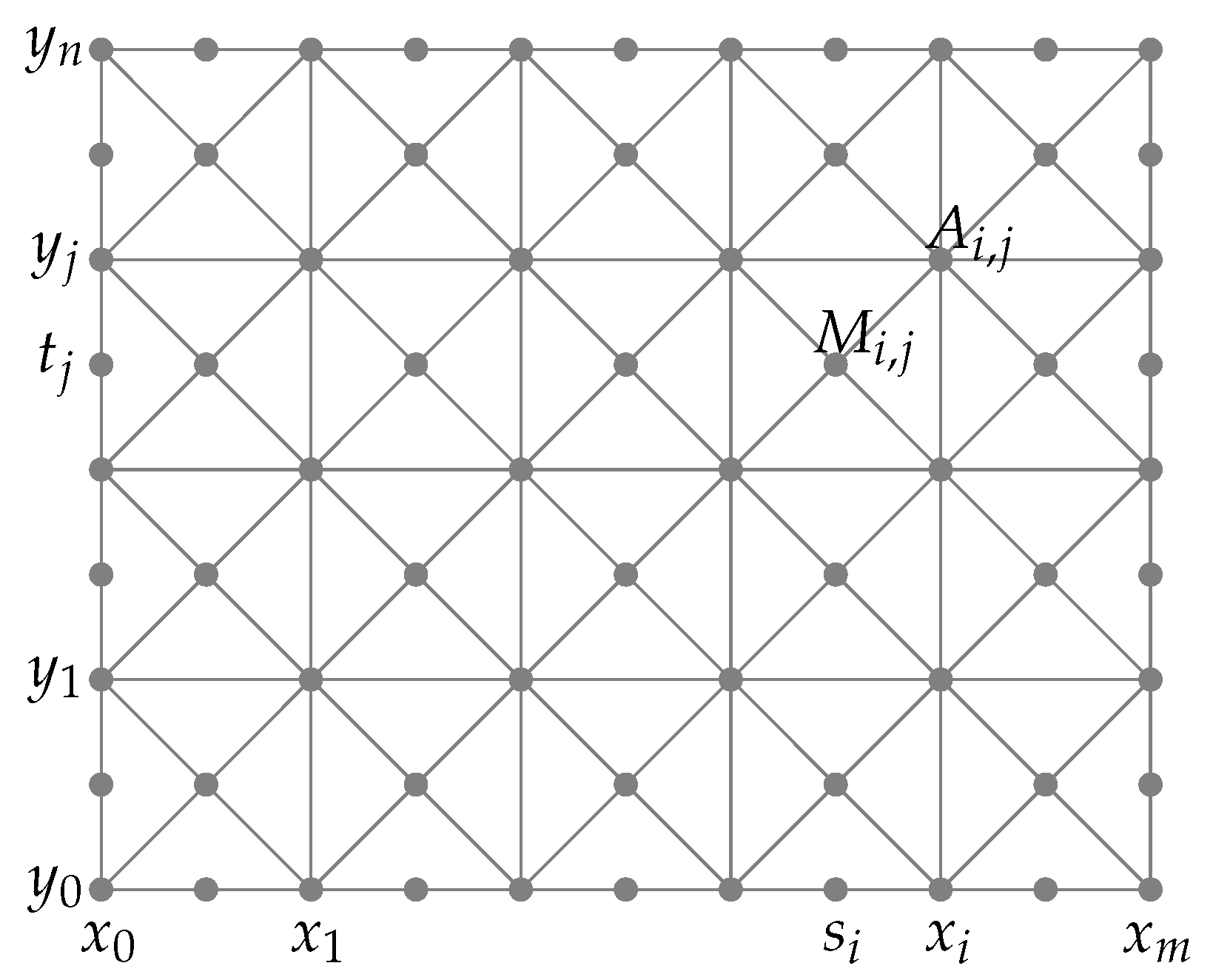
Points , , used in evaluating f, are as follows (see Figure 1):
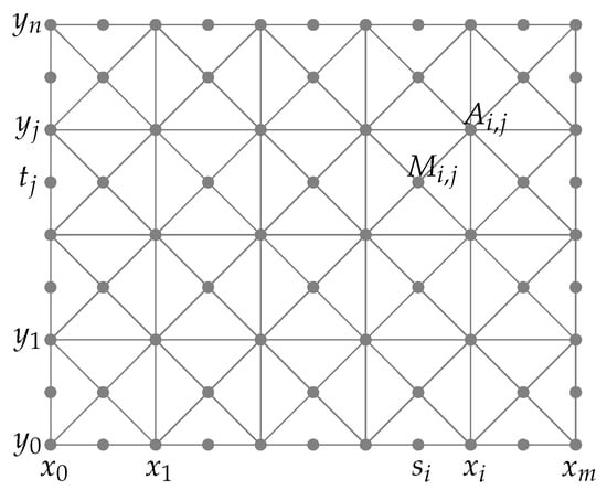
Figure 1.
Uniform criss-cross triangulation and data points.
- -
- The vertices , , of squares;
- -
- The centers , , of squares;
- -
- The midpoints of boundary segments , , , , ,
where
Moreover, we introduce the following notations: and .
Different point QIs that are exact on can be constructed using the QI nodes shown in Figure 1 (or a subset). For example, considering the following differential QI, exact on ([23] (Chapter 6)):
and by using the five-point discretization of the Laplacian , from (1), the following coefficient functionals are defined [16] (see Figure 2a)
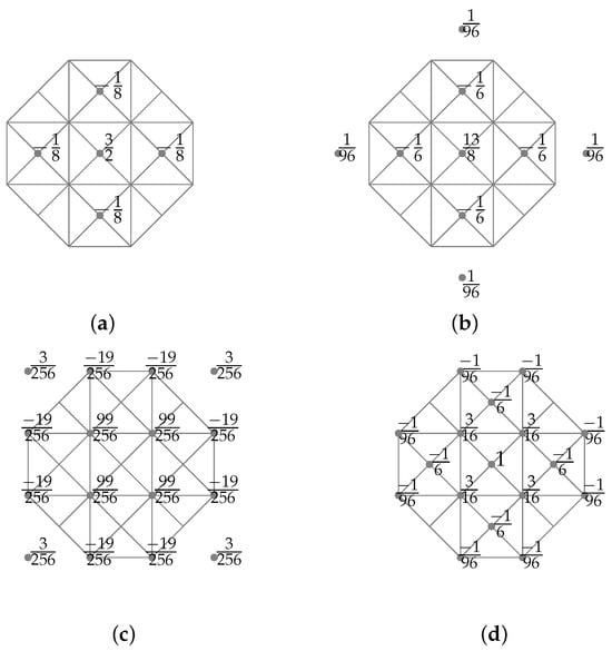
This is not the unique choice for having a point QI that is exact on . In Figure 2, other possibilities are shown; they were obtained considering other kinds of approximations for . We note that these coefficient functionals are suitable for box splines having support inside the domain, “far” from the boundary. For boundary generators, it is necessary to construct specific functionals using QI nodes inside the domain (for details, see [24], where this problem is encountered) and impose the reproduction of quadratic polynomials.
Regarding the approximation properties of such operators (see, e.g., [1,8,22]), we note that a QI has approximation order k, if
i.e., the maximum error is for , with an h-independent constant C. The maximum value of k that we can obtain, which provides optimal approximation, is related to the polynomial reproduction properties of Q. Since the above-mentioned QIs reproduce , they have the optimal approximation order 3. Also, the differential operator has the approximation order 3, i.e.,
If the function f has a jump inside , then we expect
3. WENO Techniques
In this section, we recall some definitions and properties of the WENO techniques. For more details, the reader can refer to references [25,26,27,28]. Taking into account the purposes of the paper, we assume to have different approximations (for example, five) of of this kind:
where , p, , and
for suitable values , . In general, the requirement is that can be written as the linear combination of N coefficient functionals and suitable values , .
In the case of functions f with jump discontinuity, oscillations in the approximation may occur; here, we want to apply the WENO technique to obtain a modified , which (essentially) does not produce oscillations.
If the values are positive for , we define the nonlinear coefficient functional
where
and is an indicator of the smoothness of the region that contains the values involved in the calculation of , meaning that the smoother the function f, the closer it is to zero. In particular, if f is smooth, then is as accurate as , i.e.,
Instead, if f has a discontinuity in the region where the data used by lie, but it is smooth in at least one of the regions used to calculate the , then is as accurate as , i.e.,
In the case of negative values in (3), the WENO procedure cannot be applied directly to obtain stable schemes, and it is necessary to modify the procedure; here, we propose the technique presented in [28]. So, suppose we have , where some . In this case, the nonlinear coefficient functionals are defined as
where
and
4. Nonlinear Spline Quasi-Interpolants
In this section, we construct nonlinear spline quasi-interpolants by applying the WENO techniques of Section 3 to the linear quasi-interpolants with coefficient functionals , 1, 2, 3, and 4, as shown in Figure 2.
Therefore, we consider the differential QI with coefficient functional given in (1), and the four linear QIs , 1, 2, 3, and 4, defined in this way:
with the inner functionals, as in Figure 2, and the boundary ones defined in a specific way, ensuring the reproduction of and the optimal approximation order 3. In [24], several strategies for the construction of boundary functionals are proposed and the obtained functionals can be used for defining the QIs (, , and ). For the operators, we constructed ad hoc boundary functionals satisfying the above requirements.
We apply the WENO technique only to obtain nonlinear inner functionals; for the boundary ones, we adopt a strategy that is able to avoid the Gibbs phenomenon, as explained in Section 5.
Moreover, we define the following domains
used in the subsequent subsections.
4.1. The Nonlinear Quasi-Interpolant
We want to apply the WENO technique to the operator to obtain the nonlinear analog . Thus, we decompose (see Figure 2a), as
and we recall that
Since the differential coefficient is defined by means of , we apply the WENO strategies separately in both directions x and y. Therefore, we define , ,
and we have
Taking into account the results reported in Section 3, we compute the quantities , , , we consider the smooth indicators , , , and we obtain the values , , and, consequently, the weights , , . Now, we are able to define the nonlinear coefficient functional
and the corresponding quasi-interpolant .
Theorem 1.
The following results hold:
- 1.
- is exact on the space ;
- 2.
- if f is smooth, then ;
- 3.
- if f has a discontinuity across the square , and it is smooth on and , then, ,, .
Proof.
If f is smooth, statement 2 follows by (2), (5), and (8). However, this fact does not guarantee the reproduction of . Indeed, each of the parts into which and have been subdivided, guarantee , .
Now, taking into account the definition of (see Figure 2a), if f has a discontinuity across the square , then
Within the square, , the 16 spanning functions , where and are involved, i.e., . To construct the spline within the square , we use the information on both sides of the discontinuity. However, when constructing in (and similarly in ), we only use the information on one side of the discontinuity, obtaining an approximation as a consequence of (9). The same logical scheme can be used to prove the results in .
Moreover, if the discontinuity is across the square , the region affected by the discontinuity and involved in the construction of is only and, therefore,
□
Remark 1.
If the discontinuity runs across the square , the region affected by the discontinuity in spans . It follows from the definition of , as seen in Figure 2a, and because the support of is in the square . Elsewhere in the domain, the approximation retains an order of 3.
4.2. The Nonlinear Quasi-Interpolant
The construction of the nonlinear quasi-interpolant is similar to the construction of , but in this case, we have the following (see Figure 2b):
and we recall that
Defining , and
we have
Applying the WENO technique with negative weights, considered as smooth indicators , , , we obtain
and .
Theorem 2.
The following results hold:
- 1.
- is exact on the space ;
- 2.
- if f is smooth, then ;
- 3.
- if f has a discontinuity across the square , and it is smooth on and , then , .
Proof.
If f is smooth, statement 2 follows by (2), (5), and (11). With respect to what happens for , here, the parts into which and have been subdivided guarantee , .
Now, taking into account the definition of (see Figure 2b), if f has a discontinuity across the square , then
The reasoning, as laid out in the proof of Theorem 1, is as follows: within the square , 16 spanning functions are involved, with and . When constructing in (and similarly in ), we are able to use the information only on one side of the discontinuity, obtaining an approximation as a consequence of (12). The same logical scheme can be used to prove the results in . □
Remark 2.
If the discontinuity is across the square , the region affected by the discontinuity in is . It follows from the definition of , as seen in Figure 2b, and because the support of is in the square . Elsewhere in the domain, the approximation retains an order of 3.
4.3. The Nonlinear Quasi-Interpolant
Defining , we apply the WENO technique with positive weights and, from (4), we obtain
and .
In this case, as the smooth indicator, we considered the average of the six second-order forward differences involved in the definitions of , , , .
Theorem 3.
The following results hold:
- 1.
- is exact on the space ;
- 2.
- if f is smooth, then ;
- 3.
- if f has a discontinuity across the square , and it is smooth on and , then , .
Proof.
We can prove the theorem analogously to Theorems 1 and 2. However, in this case, thanks to (14), if f has a discontinuity across the square , then
In the square , the 9 spanning functions with and are involved, i.e., ; to construct the spline within the square , we use the information from both sides of the discontinuity. However, when constructing in (and similarly in ), we only use the information on one side of the discontinuity, obtaining an approximation as a consequence of (15). The same logical scheme can be used to prove the results in . □
Remark 3.
If the discontinuity is across the square , the region affected by the discontinuity in is . It follows from the definitions of , as seen in Figure 2c, and because the support of is in the square . Elsewhere in the domain, the approximation retains an order of 3.
4.4. The Nonlinear Quasi-Interpolant
Defining , we apply the WENO technique, obtaining
and .
In this case, as the smooth indicator, we considered the average of the four second-order forward differences constructed from the points involved in the definitions of , , , .
Theorem 4.
The following results hold:
- 1.
- is exact on the space ;
- 2.
- if f is smooth, then ;
- 3.
- if f has a discontinuity across the square , and it is smooth on and , then , .
Proof.
We can prove the theorem analogously to the previous cases. Thanks to (17), if f has a discontinuity across the square , then
In the square , the 9 spanning functions , with and are involved, i.e., ; to construct the spline within the square , we use the information on both sides of the discontinuity. However, when constructing in (and similarly in ), we only use the information on one side of the discontinuity, obtaining an approximation as a consequence of (18). The same logical scheme can be used to prove the results in . □
Remark 4.
If the discontinuity is across the square , the region affected by the discontinuity in is . Elsewhere in the domain, the approximation retains an order of 3. It follows from the same arguments of Remark 3.
5. Numerical Results
In this section, we propose numerical tests confirming the theoretical results of Section 4. For each test function, we compute the maximum absolute errors
, for increasing values of m and n, using a uniform rectangular grid G of evaluation points in the domain. We also compute the corresponding numerical convergence orders (, , ), obtained by applying the base 2 logarithm to the ratio between the two consecutive errors.
Moreover, in order to only test the nonlinear modification of the quasi-interpolants, we compute the errors in a subdomain where the boundary functionals are not involved.
Finally, we provide some graphical results to confirm the reduction of the Gibbs phenomenon using the WENO technique.
Regarding the choice of the boundary functionals:
- In Tests 1 and 2, we consider ad hoc boundary functionals, ensuring the reproduction of . The boundary functionals are the same for and , for , 2, 3, and 4, respectively;
- In Tests 3 and 4, we consider ad hoc boundary functionals, ensuring the reproduction of for , , 2, 3, and 4. For the operators , , 2, 3, and 4, in order to eliminate the Gibbs phenomenon near the boundary of the domain, the boundary functionals are chosen so that the evaluation points used for their definition are located only in one sub-square of the box spline support, but ensuring an error similar to the well-known Schoenberg operator [29,30].
We tested the reproduction properties of all quasi-interpolants; we can state that all the quasi-interpolants are exact on , except , which is exact on bilinear polynomials, according to statement 1 in Theorems 1–4.
5.1. Test 1: Smooth Functions
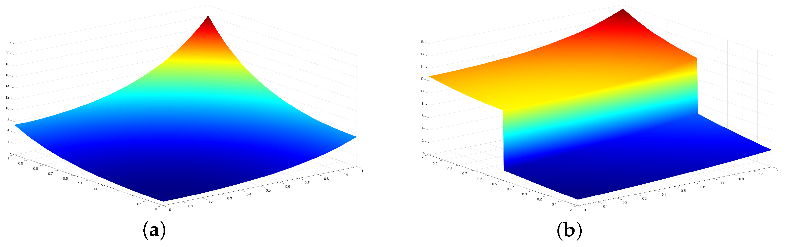
We consider the following smooth function (see Figure 3a)
and we compute the maximum absolute error in (see Table 1) and in (see Table 2), where the boundary functionals have no influence.

Figure 3.
The graphs of (a) and (b) .

Table 1.
Test 1—maximum absolute errors and numerical convergence order in .
Table 2.
Test 1—maximum absolute errors and numerical convergence order in .
We noticed that approximation order 3 was achieved by all operators, as expected from statement 2, in Theorems 1, 2, 3, and 4, respectively.
5.2. Test 2: Piecewise Smooth Function
We consider the following piecewise smooth function (see Figure 3b)
and we compare the four quasi-interpolants: , , , and , according to statement 3 in Theorems 1, 2, 3, and 4, respectively. In Table 3, we report the maximum absolute error in . We also considered the linear operators , , for which we expect an error .
Table 3.
Test 2—maximum absolute errors and numerical convergence order in .
We noticed that the expected behaviour of statement 3 in Theorems 1–4, was achieved.
5.3. Test 3: Graphical Examples
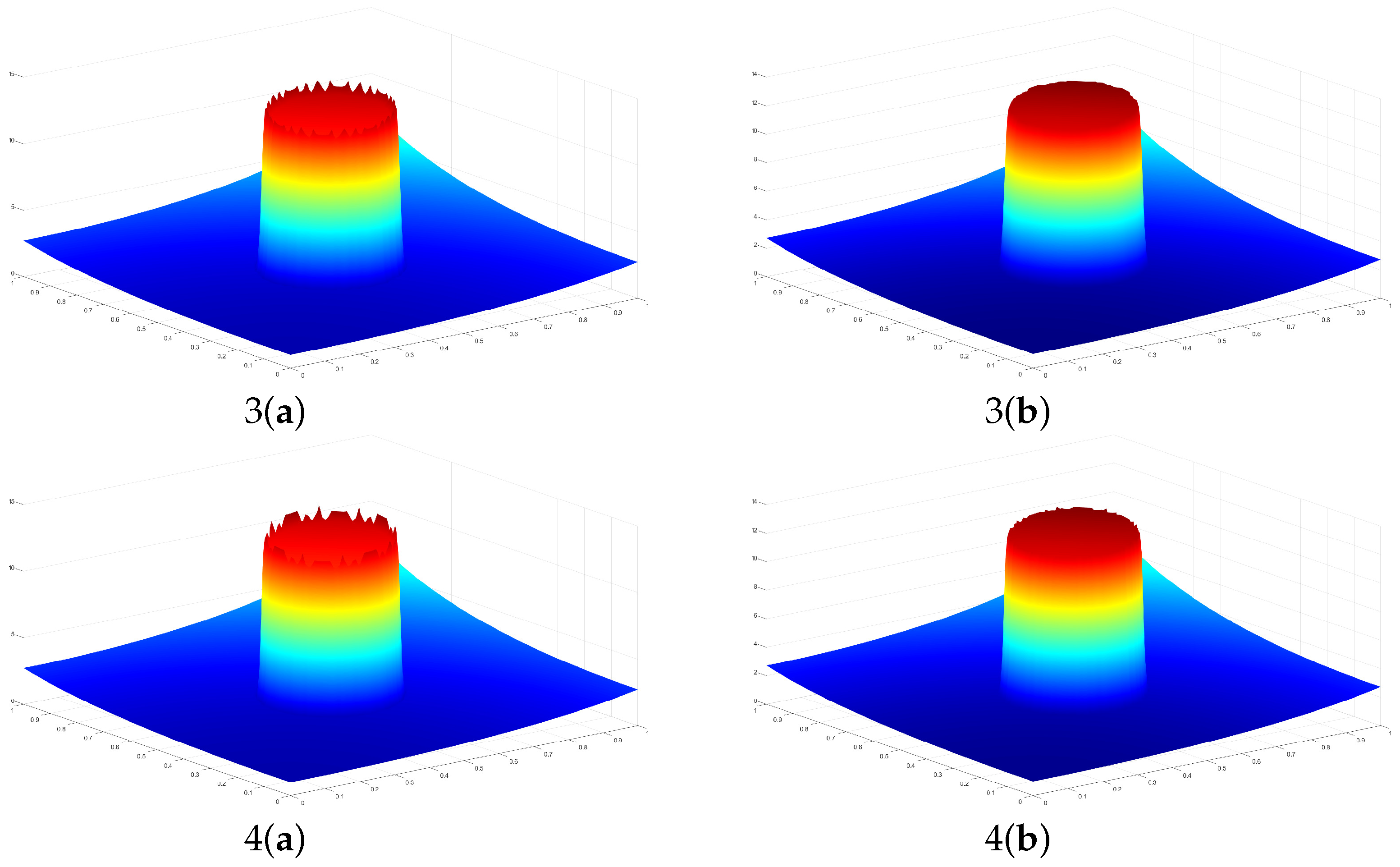
We consider the step function (see Figure 4a)
and the following piecewise smooth function (see Figure 4b)
and we compare all eight quasi-interpolants proposed in the paper from the graphical point of view.
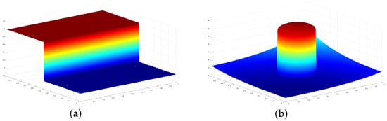
Figure 4.
The graphs of (a) and (b) .
We noticed that when using the nonlinear quasi-interpolants , where , 2, 3, and 4 (see Figure 5 (1(b)–4(b)) and Figure 6 (1(b)–4(b))), the Gibbs phenomenon is not present, with respect to the graphs obtained with the standard quasi-interpolants for , 2, 3, and 4 (see Figure 5(1(a)–4(a)) and Figure 6(1(a)–4(a))).
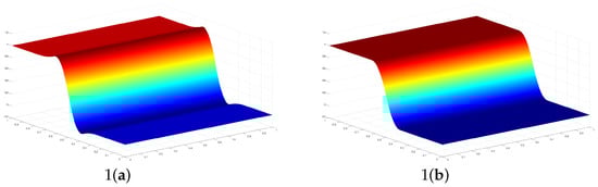
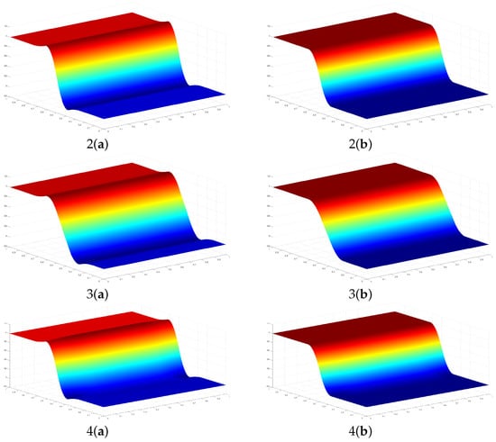
Figure 5.
The graphs of 1(a) , 1(b) , 2(a) , 2(b) , 3(a) , 3(b) and 4(a) , 4(b) , with .
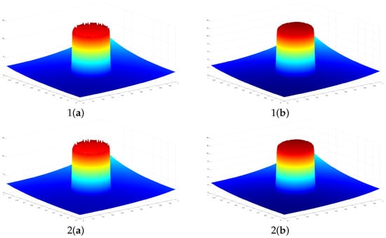
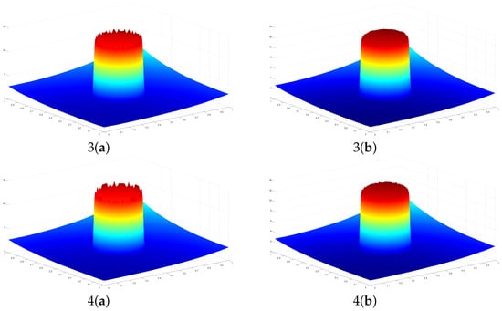
Figure 6.
The graphs of 1(a) , 1(b) , 2(a) , 2(b) , 3(a) , 3(b) and 4(a) , 4(b) , with .
6. Conclusions
In the paper, we proposed a method based on bivariate quadratic spline QIs on criss-cross triangulations for the approximation of piecewise smooth functions, obtained by modifying the coefficient functionals of the QIs by means of WENO techniques. The modified approximants are able to avoid oscillations near discontinuity and maintain high-order accuracy in smooth regions, without knowing where the discontinuity is. We also studied their convergence properties and provided several numerical and graphical tests that confirmed the theoretical results.
Author Contributions
Conceptualization, F.A. and S.R.; methodology, F.A. and S.R.; software, S.R.; validation, F.A. and S.R.; formal analysis, F.A. and S.R.; investigation, F.A. and S.R.; resources, F.A. and S.R.; data curation, F.A. and S.R.; writing—original draft preparation, F.A. and S.R.; writing—review and editing, F.A. and S.R.; visualization, F.A. and S.R.; supervision, F.A.; project administration, F.A. and S.R.; funding acquisition, F.A. All authors have read and agreed to the published version of the manuscript.
Funding
The research of the first author was supported by the Spanish MINECO project PID2020-117211GB-I00 and the GVA project CIAICO/2021/227.
Data Availability Statement
The data presented in this study are available on request to the authors.
Acknowledgments
The second author is a member of the INdAM Research group, GNCS, of Italy.
Conflicts of Interest
The authors declare no conflict of interest.
References
- Buhmann, M.; Jäger, J. Quasi-Interpolation; Cambridge University Press: Cambridge, UK, 2022. [Google Scholar]
- Ariza-López, F.J.; Barrera, D.; Eddargani, S.; Ibañez, M.J.; Reinoso, J.F. Spline quasi-interpolation in the Bernstein basis and its application to digital elevation models. Math. Methods Appl. Sci. 2023, 46, 1687–1698. [Google Scholar] [CrossRef]
- Gao, W.; Wang, J.; Zhang, R. Quasi-interpolation for multivariate density estimation on bounded domain. Math. Comput. Simul. 2023, 203, 592–608. [Google Scholar] [CrossRef]
- Rahimi, M.; Adibi, H.H.; Amirfakhrian, M. Numerical study of nonlinear generalized Burgers-Huxley equation by multiquadric quasi-interpolation and pseudospectral method. Math. Sci. 2023, 17, 431–444. [Google Scholar] [CrossRef]
- Sun, Z.; Gao, W.; Yang, R. A Convergent Iterated Quasi-interpolation for Periodic Domain and Its Applications to Surface PDEs. J. Sci. Comput. 2022, 93, 37. [Google Scholar] [CrossRef]
- Aràndiga, F.; Donat, R.; López-Ureña, S. Nonlinear improvements of quasi-interpolant splines to approximate piecewise smooth functions. Appl. Math. Comp. 2023, 448, 127946. [Google Scholar] [CrossRef]
- Amat, S.; Levin, D.; Ruiz-Álvarez, J.; Trillo, J.C.; Yáñez, D.F. A class of C2 quasi-interpolating splines free of Gibbs phenomenon. Num. Algor. 2022, 91, 51–79. [Google Scholar] [CrossRef]
- de Boor, C.; Höllig, K.; Riemenschneider, S. Box Splines; Springer: New York, NY, USA, 1993. [Google Scholar]
- Wang, R.H. Multivariate Spline Functions and Their Application; Science Press: Beijing, China; New York, NY, USA; Kluwer Academic Publishers: Dordrecht, Germany; Boston, MA, USA; London, UK, 2001. [Google Scholar]
- Barrera, D.; Ibañez, M.J.; Sablonnière, P.; Sbibih, D. On near-best discrete quasi-interpolation on a four-directional mesh. J. Comput. Appl. Math. 2010, 233, 1470–1477. [Google Scholar] [CrossRef]
- Chui, C.K.; Wang, R.H. On a bivariate B-splines basis. Sci. Sin. (Ser. A) 1984, XXVI, 1129–1142. [Google Scholar]
- Dagnino, C.; Lamberti, P. On the approximation power of bivariate quadratic C1 splines. J. Comput. Appl. Math. 2001, 131, 321–332. [Google Scholar] [CrossRef]
- Dagnino, C.; Lamberti, P. On the construction of local quadratic spline quasi-interpolants on bounded rectangular domains. J. Comput. Appl. Math. 2008, 221, 367–375. [Google Scholar] [CrossRef]
- Dagnino, C.; Remogna, S.; Sablonnière, P. Error bounds on the approximation of functions and partial derivatives by quadratic spline quasi-interpolants on non-uniform criss-cross triangulations of a rectangular domain. BIT Numer. Math. 2013, 53, 87–109. [Google Scholar] [CrossRef]
- Sablonnière, P. Bernstein-Bézier methods for the construction of bivariate spline approximants. Comput. Aided Geom. Des. 1985, 2, 29–36. [Google Scholar] [CrossRef]
- Sablonnière, P. On some multivariate quadratic spline quasi-interpolants on bounded domains. In Proceedings of the Modern Developments in Multivariate Approximation: 5th International Conference, Witten-Bommerholz, Germany, 22–27 September 2002; Birkhäuser: Basel, Switzerland, 2003; pp. 263–278. [Google Scholar]
- Wang, R.H.; Li, C.J. A kind of multivariate NURBS surfaces. J. Comp. Math. 2004, 22, 137–144. [Google Scholar]
- Conchin-Gubernati, A.; Lamberti, P. Multilevel quadratic spline integration. J. Comput. Appl. Math. 2022, 407, 114057. [Google Scholar] [CrossRef]
- Lamberti, P.; Saponaro, A. Multilevel quadratic spline quasi-interpolation. Appl. Math. Comp. 2020, 373, 125047. [Google Scholar] [CrossRef]
- Qian, J.; Shi, X.; Wu, J.; Gong, D. Construction of cubature formulas via bivariate quadratic spline spaces over non-uniform type-2 triangulation. J. Comput. Appl. Math. 2022, 40, 206–231. [Google Scholar] [CrossRef]
- Dagnino, C.; Lamberti, P.; Remogna, S. B-spline bases for unequally smooth quadratic spline spaces on non-uniform criss-cross triangulations. Num. Algor. 2012, 61, 209–222. [Google Scholar] [CrossRef]
- Chui, C.K. Multivariate Splines; CBMS-NSF Regional Conference Series in Applied Mathematics; SIAM: Philadelphia, PA, USA, 1988; Volume 54. [Google Scholar]
- Sablonnière, P. Bases de Bernstein et Approximants Splines. Ph.D. Thesis, Université de Lille, Lille, France, 1982. [Google Scholar]
- Remogna, S. Constructing Good Coefficient Functionals for Bivariate C1 Quadratic Spline Quasi-Interpolants. In Proceedings of the Mathematical Methods for Curves and Surfaces: 7th International Conference, MMCS 2008, Tønsberg, Norway, 26 June–1 July 2008; Revised Selected Papers 7; Springer: Berlin/Heidelberg, Germany, 2010; pp. 329–346. [Google Scholar]
- Aràndiga, F.; Baeza, A.; Belda, A.M.; Mulet, P. Analysis of WENO schemes for full and global accuracy. SIAM J. Numer. Anal. 2011, 49, 893–915. [Google Scholar] [CrossRef]
- Aràndiga, F.; Belda, A.M.; Mulet, P. Point-value WENO multiresolution applications to stable image compression. J. Sci. Comp. 2010, 43, 158–182. [Google Scholar] [CrossRef]
- Jiang, G.S.; Shu, C.W. Efficient implementation of weighted ENO schemes. J. Comput. Phys. 1996, 126, 202–228. [Google Scholar] [CrossRef]
- Shi, J.; Hu, C.; Shu, C.W. A technique of treating negative weights in WENO schemes. J. Comput. Phys. 2002, 175, 108–127. [Google Scholar] [CrossRef]
- Schoenberg, I.J. Contributions to the problem of approximation of equidistant data by analytic functions. Part A. On the problem of smoothing or graduation. A first class of analytic approximation formulae. Quart. Appl. Math. 1946, 4, 45–99. [Google Scholar] [CrossRef]
- Schoenberg, I.J. Contributions to the problem of approximation of equidistant data by analytic functions. Part B. On the problem of osculatory interpolation, a second class of analytic approximation formulae. Quart. Appl. Math. 1946, 4, 112–141. [Google Scholar] [CrossRef]


Disclaimer/Publisher’s Note: The statements, opinions and data contained in all publications are solely those of the individual author(s) and contributor(s) and not of MDPI and/or the editor(s). MDPI and/or the editor(s) disclaim responsibility for any injury to people or property resulting from any ideas, methods, instructions or products referred to in the content. |
© 2023 by the authors. Licensee MDPI, Basel, Switzerland. This article is an open access article distributed under the terms and conditions of the Creative Commons Attribution (CC BY) license (https://creativecommons.org/licenses/by/4.0/).