A Game—Theoretic Model for a Stochastic Linear Quadratic Tracking Problem

Abstract

In this paper, we solve a stochastic linear quadratic tracking problem. The controlled dynamical system is modeled by a system of linear Itô differential equations subject to jump Markov perturbations. We consider the case when there are two decision-makers and each of them wants to minimize the deviation of a preferential output of the controlled dynamical system from a given reference signal. We assume that the two decision-makers do not cooperate. Under these conditions, we state the considered tracking problem as a problem of finding a Nash equilibrium strategy for a stochastic differential game. Explicit formulae of a Nash equilibrium strategy are provided. To this end, we use the solutions of two given terminal value problems (TVPs). The first TVP is associated with a hybrid system formed by two backward nonlinear differential equations coupled by two algebraic nonlinear equations. The second TVP is associated with a hybrid system formed by two backward linear differential equations coupled by two algebraic linear equations.

1. Introduction

Tracking problems are often encountered in many applications and have received attention from the research community in the past few decades [1,2,3,4,5]. In the stochastic context, this problem was studied in [6,7] as well as in [8,9]. For stochastic systems with time delay, the linear quadratic tracking problem has been studied in [10,11]. Applications of tracking problems may be found in economic policy control [12], process control [13], networked control systems [14], control of mobile robots [15], spacecraft hovering [16], etc. Usually, a linear quadratic tracking problem requires minimization of the $L_2$-norm of the deviation of a signal generated by a controlled linear system from a reference signal. When there exists more than one decision maker and each of them wants to minimize the deviation of a preferential signal from a given reference signal, the optimal tracking problem may be stated as a problem of finding a Nash equilibrium strategy for a linear quadratic differential game. If the controlled system whose outputs have to track the given reference signal is described by linear stochastic differential equations, one obtains a problem of finding a Nash equilibrium strategy for a stochastic differential game. Lately, the stochastic differential games have attracted an increasing research interest see, e.g., [17,18,19,20]. Moreover, for Nash tracking game problems for continuous-time systems over finite intervals see [21] and the reference therein.

In the present work, we consider the case when the controlled system is described by a system of Itô differential equations with coefficients affected by a standard homogeneous Markov process with a finite number of states. We assume that there exist at least two decision-makers. The aim of the k-th decision-maker is to minimize the deviation of an output $z_k(·)$ of the controlled system from a reference signal $r_k(·)$. The class of admissible strategies consists of stochastic processes in an affine state feedback form.

In the derivation of the main results we consider two cases:

(a) the case with only one decision-maker;

(b) the case of two decision-makers.

The result derived from case (a) is used in the case with more than one decision-maker in order to obtain an optimal strategy. In case (b), we study the game theoretic model for two players, where each player wants to find the optimal admissible strategy minimizing the deviation of the controlled signal from the given reference.

We assume that the players do not cooperate. The reasons for which they are not cooperating may be caused by individual motivations or by physical reasons. We provide explicit formulae of a Nash equilibrium strategy. To this end, we use the solutions of two TVPs. The first TVP is associated with a hybrid system formed by two backward nonlinear differential equations coupled with two algebraic nonlinear equations. The second TVP is associated with a hybrid system formed by two backward linear differential equations coupled by two algebraic linear equations.

The paper is organized as follows: Section 2 includes the description of the mathematical model as well as the formulation of the tracking problem as a problem of finding a Nash equilibrium strategy for a stochastic differential game. The main results are derived in Section 3. First, in Section 3.1, we consider the case with one decision-maker. Further, in Section 3.2, we obtain explicit formulae for the optimal strategies in the case of two decision-makers. In Section 4, we briefly discuss two special cases: (i) the case when the controlled system does not contain controlled dependent terms in the diffusion part; (ii) the case when the aim of the decision-makers is to minimize the deviation of the controlled signals from a given final target without restrictions regarding the behavior of the transient states. In Section 5, we provide a numerical example that shows that the proposed procedure is feasible. Finally, in Section 6, we provide some conclusions and future research directions.

2. The Problem

Consider the controlled system having the state space representation described by

$$\begin{array}{cc}\hfill & dx\left(t\right)=[A_0(t,{\eta }_t)x\left(t\right)+B_1(t,{\eta }_t)u_1\left(t\right)+B_2(t,{\eta }_t)u_2\left(t\right)]dt\hfill \\ \hfill & +[A_1(t,{\eta }_t)x\left(t\right)+D_1(t,{\eta }_t)u_1\left(t\right)+D_2(t,{\eta }_t)u_2\left(t\right)]dw\left(t\right),\hfill \end{array}$$

$$\begin{array}{cc}\hfill & x\left(t_0\right)=x_0,\hfill \end{array}$$

(1a)

$$\begin{array}{cc}\hfill & z_k\left(t\right)=C_k(t,{\eta }_t)x\left(t\right),k=1,2,\hfill \end{array}$$

(1b)

$t\in [t_0,t_f]\subset [0,\infty ),$ where $x\left(t\right)\in {\mathbb{R}}^n$ is the state vector at instance time t and $u_k\left(t\right)\in {\mathbb{R}}^{m_k},$ $k=1,2,$ are the vectors of control parameters. In (1), ${\left\{w\left(t\right)\right\}}_{t\ge 0},$ is a one-dimensional standard Wiener process defined on a given probability space $(\Omega ,\mathcal{F},\mathcal{P})$ and ${\left\{{\eta }_t\right\}}_{t\ge 0}$ is a standard right continuous Markov process taking values in a finite set $\mathcal{N}=\{1,2,\dots ,N\}$ and having the transition semigroup $\mathbb{P}\left(t\right)=e^{Qt},$ $t\ge 0.$ The elements $q_{ij}$ of the generator matrix $Q\in {\mathbb{R}}^{N\times N}$ satisfy

$$\begin{array}{cc}\hfill & q_{ij}\ge 0\mathrm{if}i\ne j,\hfill \end{array}$$

(2a)

$$\begin{array}{cc}\hfill & \sum _{l=1}^N{q}_{il}=0,\hfill \end{array}$$

(2b)

for all $(i,j)\in \mathcal{N}\times \mathcal{N}$. For more details regarding the properties of a Wiener process, one can see [22] or [23], whereas for more properties of a Markov process, we refer, for example, to [24,25].

Throughout the paper, we assume that ${\left\{w\left(t\right)\right\}}_{t\ge 0}$ and ${\left\{{\eta }_t\right\}}_{t\ge 0}$ are independent stochastic processes. The dependence of the coefficients of the system (1) upon the Markov process ${\left\{{\eta }_t\right\}}_{t\ge 0}$ highlights the fact that this system may be considered the mathematical model of some phenomena in which abrupt structural changes are likely to occur. Such variations may be due, for instance, to changes between different operation points, sensor or actuator failures, temporary loss of communication, and so on. For the readers’ convenience, we refer to [9,26,27,28] for extensive discussions on the subject. As usual, we shall write $A_k(t,i),$ $k=0,1,$ $B_j(t,i),$ $C_j(t,i),$ $D_j(t,i),$ $j=1,2$ instead of $A_k(t,{\eta }_t),$ and so on, whenever ${\eta }_t=i\in \mathcal{N}.$ Assume that $t\to A_k(t,i):[t_0,t_f]\to {\mathbb{R}}^{n\times n},$ $k=0,1,$ $t\to (B_j(t,i),C_j(t,i),D_j(t,i)):[t_0,t_f]\to {\mathbb{R}}^{n\times m_j}\times {\mathbb{R}}^{n_{z_j}\times n}\times {\mathbb{R}}^{n\times m_j},$ $j=1,2$ are continuous matrix-valued functions. The set ${\mathcal{U}}_k$ of the admissible controls available to the decision-makers ${\mathcal{P}}_k,$ $k=1,2,$ consists of the stochastic processes in an affine state feedback form, i.e.,

$$u_k\left(t\right)=F_k(t,{\eta }_t)x\left(t\right)+{\phi }_k(t,{\eta }_t)$$

(3)

where $t\to F_k(t,i):[t_0,t_f]\to {\mathbb{R}}^{m_k\times n}$ and $t\to {\phi }_k(t,i):[t_0,t_f]\to {\mathbb{R}}^{m_k}$ are arbitrary continuous functions. Applying Theorem 1.1 in Chapter 5 from [22] (see also Section 1.12 from [9]) we obtain:

Corollary 1. 

For each $x_0\in {\mathbb{R}}^n$ and for each $u(·)=(u_1(·),u_2(·))\in {\mathcal{U}}_1\times {\mathcal{U}}_2,$ the initial value problem (IVP) (1a) has a unique solution $x_u(·;t_0,x_0)$ which is a stochastic process with the properties

(a) 

$x_u(·;t_0,x_0)$ is a.s. continuous in every $t\in [t_0,t_f];$

(b) 

for each $t\in [t_0,t_f],$ $x_u(t;t_0,x_0)$ is ${\mathcal{F}}_t-$measurable, where ${\mathcal{F}}_t\subset \mathcal{F}$ is the $\sigma -$algebra generated by the random variables $w\left(s\right),$ ${\eta }_s,$ $0\le s\le t;$

(c) 

$\underset{t\in [t_0,t_f]}{sup}\mathbb{E}\left[\right|x_u(t;t_0,x_0){|}^p]<\infty ,$ for all $p\ge 1;$

(d) 

$x_u(t_0;t_0,x_0)=x_0.$

Throughout this work, $\mathbb{E}[·]$ stands for the mathematical expectation. Roughly speaking, the aim of the decision-maker ${\mathcal{P}}_k$ is to find a control law (or an admissible strategy) of type (3), ${\tilde{u}}_k(·)\in {\mathcal{U}}_k$ which minimizes the deviation of the signal $z_k(·)$ from a given reference signal $r_k(·),$ when the other decision-maker ${\mathcal{P}}_l$ wants to minimize the deviation of the signal $z_l(·),$ $(l\ne k)$ from another reference signal $r_l(·).$

Since this problem is an optimization problem with two objective functions, its solution can be viewed as an equilibrium strategy for a non-cooperative differential game with two players. For a rigorous mathematical setting of this optimization problem, let us introduce the following cost functions which are modeling the performance criterion for each player $(k=1,2)$:

$$\begin{array}{cc}\hfill J_k(x_0;u_1(·),u_2(·))=& \mathbb{E}\left[{(z_k\left(t_f\right)-{\zeta }_k)}^T{G}_k\left({\eta }_{t_f}\right)(z_k\left(t_f\right)-{\zeta }_k)\right]\hfill \\ \hfill & +\mathbb{E}\left[\underset{t_0}{\overset{t_f}{\int }}\{{(z_k\left(t\right)-r_k\left(t\right))}^T{M}_k(t,{\eta }_t)(z_k\left(t\right)-r_k\left(t\right))\right.\hfill \\ \hfill & \left.+u_1^T\left(t\right)R_{k1}(t,{\eta }_t)u_1\left(t\right)+u_2^T\left(t\right)R_{k2}(t,{\eta }_t)u_2\left(t\right)\}dt\right].\hfill \end{array}$$

(4)

Here $r_k(·):[t_0,t_f]\to {\mathbb{R}}^{n_{z_k}},$ $k=1,2$ is the reference which must be tracked by the signal $z_k(·),$ and ${\zeta }_k\in {\mathbb{R}}^{n_{z_k}},$ $k=1,2$ is the target of the final value $z_k\left(t_f\right).$ The weight matrices involved in (4) are satisfying the assumption:

Hypothesis 1. 

(a) 

$t\to (M_k(t,i),R_{k1}(t,i),R_{k2}(t,i)):[t_0,t_f]\to {\mathcal{S}}_{n_{z_k}}\times {\mathcal{S}}_{m_1}\times {\mathcal{S}}_{m_2},$ $i\in \mathcal{N}$ are continuous matrix-valued functions;

(b) 

$M_k(t,i)\ge 0,$ $R_{kl}(t,i)\ge 0,$ $R_{kk}(t,i)>0,$ for all $t\in [t_0,t_f],$ $k,l=1,2,$ $l\ne k,$ $G_k\left(i\right)\ge 0,$ $i\in \mathcal{N}.$

Here and in the sequel, ${\mathcal{S}}_p\subset {\mathbb{R}}^{p\times p}$ denotes the subspace of symmetric matrices of size $p\times p,$ $p\ge 1.$

Definition 1. 

We say that the pair of admissible strategies $({\tilde{u}}_1(·),{\tilde{u}}_2(·))\in {\mathcal{U}}_1\times {\mathcal{U}}_2$ achieve a Nash equilibrium for the differential game described by the controlled system (1), the performance criterion (4), and the admissible strategies of type (3) if

$$J_1(x_0;{\tilde{u}}_1(·),{\tilde{u}}_2(·))\le J_1(x_0;u_1(·),{\tilde{u}}_2(·)),forall{u}_1\in {\mathcal{U}}_1$$

(5)

and

$$J_2(x_0;{\tilde{u}}_1(·),{\tilde{u}}_2(·))\le J_2(x_0;{\tilde{u}}_1(·),u_2(·)),forall{u}_2\in {\mathcal{U}}_2.$$

(6)

In the next section, we shall derive explicit formulae of a Nash equilibrium strategy $({\tilde{u}}_1(·),{\tilde{u}}_2(·))$ for the linear quadratic differential game described by (1), (3), and (4).

Remark 1.

(a) 

We shall see that for the computation of the gain matrices of a Nash equilibrium strategy we need to know a priori the whole reference signal $r_k(·).$

(b) 

When $M_k(t,i)=0,$ for all $(t,i)\in [t_0,t_f]\times \mathcal{N},$ then (4) reduces to

$$\begin{array}{cc}\hfill & J_k(x_0;u_1(·),u_2(·))=\mathbb{E}\left[{(z_k\left(t_f\right)-{\zeta }_k)}^T{G}_k\left({\eta }_{t_f}\right)(z_k\left(t_f\right)-{\zeta }_k)\right]\hfill \\ \hfill & +\mathbb{E}\left[\underset{t_0}{\overset{t_f}{\int }}\{u_1^T\left(t\right)R_{k1}(t,{\eta }_t)u_1\left(t\right)+u_2^T\left(t\right)R_{k2}(t,{\eta }_t)u_2\left(t\right)\}dt\right],k=1,2.\hfill \end{array}$$

(7)

The performance criterion (4) could be replaced by one of the form (7), when the decision-maker is interested only by the minimization of the deviation of the final value $z_k\left(t_f\right)$ from the target ${\zeta }_k.$ The term

$$\mathbb{E}\left[\underset{t_0}{\overset{t_f}{\int }}\{u_1^T\left(t\right)R_{k1}(t,{\eta }_t)u_1\left(t\right)+u_2^T\left(t\right)R_{k2}(t,{\eta }_t)u_2\left(t\right)\}dt\right],$$

which appears both in (4) and (7), must be viewed as a penalization of the control effort.

3. The Main Results

3.1. The Case with Only One Decision Maker

In order to derive in an elegant way the state space representation of a pair of form (3) which satisfies (5) and (6), respectively, we study first the problem of tracking a reference signal in the case where there is only one decision maker.

We consider the optimal control problem described by the controlled system:

$$\begin{array}{cc}\hfill & dx\left(t\right)=[A_0(t,{\eta }_t)x\left(t\right)+B(t,{\eta }_t)u\left(t\right)+g_0(t,{\eta }_t)]dt\hfill \\ \hfill & +[A_1(t,{\eta }_t)x\left(t\right)+D(t,{\eta }_t)u\left(t\right)+g_1(t,{\eta }_t)]dw\left(t\right),\hfill \end{array}$$

$$\begin{array}{cc}\hfill & x\left(t_0\right)=x_0,\hfill \end{array}$$

(8a)

$$\begin{array}{cc}\hfill & z\left(t\right)=C(t,{\eta }_t)x\left(t\right),\hfill \end{array}$$

(8b)

$t\in [t_0,t_f]$ and the performance criterion

$$\begin{array}{cc}\hfill J(x_0;u(·))=& \mathbb{E}\left[{(z\left(t_f\right)-\zeta )}^{T}G\left({\eta }_{t_f}\right)(z\left(t_f\right)-\zeta )\right]\hfill \\ \hfill & +\mathbb{E}\left[\underset{t_0}{\overset{t_f}{\int }}\{{(z\left(t\right)-r\left(t\right))}^{T}M(t,{\eta }_t)(z\left(t\right)-r\left(t\right))+u^T\left(t\right)R(t,{\eta }_t)u\left(t\right)\}dt\right].\hfill \end{array}$$

(9)

Here, the stochastic processes ${\left\{w\left(t\right)\right\}}_{t\ge 0}$ and ${\left\{{\eta }_t\right\}}_{t\ge 0}$ have the same properties as in the case of system (1). In (8) and (9), $x\left(t\right)\in {\mathbb{R}}^n$ is the state vector at the instance time t and $u\left(t\right)\in {\mathbb{R}}^m$ is the vector of the control parameters.

In this subsection, the set $\mathcal{U}$ of admissible controls consists of stochastic processes of the form

$$u\left(t\right)=F(t,{\eta }_t)x\left(t\right)+\phi (t,{\eta }_t),$$

(10)

$t\to F(t,i):[t_0,t_f]\to {\mathbb{R}}^{m\times n},$ $t\to \phi (t,i):[t_0,t_f]\to {\mathbb{R}}^m$ which are arbitrary continuous functions. The optimal control problem which we want to solve in this subsection consists in finding a control $\tilde{u}(·)$ from $\mathcal{U}$ which minimizes the cost function (9) along the trajectories of the system (8) determined by all admissible controls of the form (10).

Regarding the coefficients of (8) and (9), we suppose:

Hypothesis 2.

(a) 

$t\to (A_0(t,i),A_1(t,i),B(t,i),D(t,i),C(t,i),M(t,i),R(t,i)):[t_0,t_f]\to {\mathbb{R}}^{n\times n}\times {\mathbb{R}}^{n\times n}\times {\mathbb{R}}^{n\times m}\times {\mathbb{R}}^{n\times m}\times {\mathbb{R}}^{n_z\times n}\times {\mathcal{S}}_{n_z}\times {\mathcal{S}}_m,$ $t\to g_k(t,i):[t_0,t_f]\to {\mathbb{R}}^n,$ $k=0,1,$ $t\to r\left(t\right):[t_0,t_f]\to {\mathbb{R}}^{n_z}$ are continuous matrix-valued functions;

(b) 

$M(t,i)\ge 0,$ $R(t,i)>0,$ for all $t\in [t_0,t_f],$ $G\left(i\right)\ge 0,$ $i\in \mathcal{N}.$

Let us consider the function $V:[t_0,t_f]\times {\mathbb{R}}^n\times \mathcal{N}\to \mathbb{R}$ defined by

$$V(t,x,i)=x^{T}X(t,i)x-2x^T\Psi (t,i)+\mu (t,i)$$

(11)

where $t\to (X(t,i),\Psi (t,i),\mu (t,i)):[t_0,t_f]\to {\mathcal{S}}_n\times {\mathbb{R}}^n\times \mathbb{R},$ $i\in \mathcal{N}$ are continuous and differentiable functions. Applying the Itô formula, see for example Theorem 1.10.2 from [9] in the case of the function (11) and to the stochastic process $x\left(t\right)$ satisfying (8a), we obtain

$$\begin{array}{cc}\hfill & \mathbb{E}[V(t_f,x\left(t_f\right),{\eta }_{t_f})-V(t_0,x\left(t_0\right),{\eta }_{t_0})|{\eta }_{t_0}=i]\hfill \\ \hfill & =\mathbb{E}\left[\underset{t_o}{\overset{t_f}{\int }}{\left(\begin{array}{c}x\left(t\right)\\ 1\\ u\left(t\right)\end{array}\right)}^T\left(\begin{array}{ccc}{W}_{11}(t,{\eta }_t)& W_{12}(t,{\eta }_t)& W_{13}(t,{\eta }_t)\\ W_{12}^T(t,{\eta }_t)& W_{22}(t,{\eta }_t)& W_{23}(t,{\eta }_t)\\ W_{13}^T(t,{\eta }_t)& W_{23}^T(t,{\eta }_t)& W_{33}(t,{\eta }_t)\end{array}\right)\left(\begin{array}{c}x\left(t\right)\\ 1\\ u\left(t\right)\end{array}\right)dt|{\eta }_{t_0}=i\right]\hfill \end{array}$$

(12)

for all $i\in \mathcal{N},$ where

$$\begin{array}{cc}\hfill & W_{11}(t,i)=\dot{X}(t,i)+A_0^T(t,i)X(t,i)+X(t,i)A_0(t,i)\hfill \end{array}$$

$$\begin{array}{cc}\hfill & +A_1^T(t,i)X(t,i)A_1(t,i)+\sum _{j=1}^N{q}_{ij}X(t,j)\hfill \\ \hfill & W_{12}(t,i)=-\dot{\Psi }(t,i)-A_0^T(t,i)\Psi (t,i)+X(t,i)g_0(t,i)\hfill \end{array}$$

(13a)

$$\begin{array}{cc}\hfill & +A_1^T(t,i)X(t,i)g_1(t,i)+\sum _{j=1}^N{q}_{ij}\Psi (t,j)\hfill \end{array}$$

(13b)

$$\begin{array}{cc}\hfill & W_{13}(t,i)=X(t,i)B(t,i)+A_1^T(t,i)X(t,i)D(t,i)\hfill \end{array}$$

(13c)

$$\begin{array}{cc}\hfill & W_{22}(t,i)=\dot{\mu }(t,i)+\sum _{j=1}^N{q}_{ij}\mu (t,j)+g_1^T(t,i)X(t,i)g_1(t,i)-2g_0^T(t,i)\Psi (t,i)\hfill \end{array}$$

(13d)

$$\begin{array}{cc}\hfill & W_{23}(t,i)=-{\Psi }^T(t,i)B(t,i)+g_1^T(t,i)X(t,i)D(t,i)\hfill \end{array}$$

(13e)

$$\begin{array}{cc}\hfill & W_{33}(t,i)=D^T(t,i)X(t,i)D(t,i)\hfill \end{array}$$

(13f)

Taking the expectation in (12) and adding with (9) we obtain

$$\begin{array}{cc}\hfill & J(x_0,u(·))+\mathbb{E}\left[V(t_f,x\left(t_f\right),{\eta }_{t_f})\right]-\mathbb{E}\left[V(t_0,x_0,{\eta }_{t_0})\right]\hfill \\ \hfill & =\mathbb{E}\left[{(x\left(t_f\right)-\zeta )}^{T}G\left({\eta }_{t_f}\right)(z\left(t_f\right)-\zeta )\right]\hfill \\ \hfill & +\mathbb{E}\left[\underset{t_o}{\overset{t_f}{\int }}{\left(\begin{array}{c}x\left(t\right)\\ 1\\ u\left(t\right)\end{array}\right)}^T\left(\begin{array}{ccc}{\widehat{W}}_{11}(t,{\eta }_t)& {\widehat{W}}_{12}(t,{\eta }_t)& {\widehat{W}}_{13}(t,{\eta }_t)\\ {\widehat{W}}_{12}^T(t,{\eta }_t)& {\widehat{W}}_{22}(t,{\eta }_t)& {\widehat{W}}_{23}(t,{\eta }_t)\\ {\widehat{W}}_{13}^T(t,{\eta }_t)& {\widehat{W}}_{23}^T(t,{\eta }_t)& {\widehat{W}}_{33}(t,{\eta }_t)\end{array}\right)\left(\begin{array}{c}x\left(t\right)\\ 1\\ u\left(t\right)\end{array}\right)dt\right]\hfill \end{array}$$

(14)

where

$$\begin{array}{cc}\hfill & {\widehat{W}}_{11}(t,i)=W_{11}(t,i)+C^T(t,i)M(t,i)C(t,i)\hfill \end{array}$$

(15a)

$$\begin{array}{cc}\hfill & {\widehat{W}}_{12}(t,i)=W_{12}(t,i)-C^T(t,i)M(t,i)r(t,i)\hfill \end{array}$$

(15b)

$$\begin{array}{cc}\hfill & {\widehat{W}}_{13}(t,i)=W_{13}(t,i)\hfill \end{array}$$

(15c)

$$\begin{array}{cc}\hfill & {\widehat{W}}_{22}(t,i)=W_{22}(t,i)+r^T(t,i)M(t,i)r(t,i)\hfill \end{array}$$

(15d)

$$\begin{array}{cc}\hfill & {\widehat{W}}_{23}(t,i)=W_{23}(t,i)\hfill \end{array}$$

(15e)

$$\begin{array}{cc}\hfill & {\widehat{W}}_{33}(t,i)=R(t,i)+D^T(t,i)X(t,i)D(t,i)\hfill \end{array}$$

(15f)

Let

$$\mathbf{X}(·)=\left(X\right(·,1),X(·,2),\dots ,X(·,N\left)\right),$$

$$\mathbf{\Psi }(·)=(\Psi (·,1),\Psi (·,2),\dots ,\Psi (·,N\left)\right),$$

$$\mathbf{\mu }(·)={(\mu (·,1),\mu (·,2),\dots ,\mu (·,N))}^T$$

be the solutions of the following terminal value problem (TVP)

$$\begin{array}{cc}\hfill & \dot{X}(t,i)+A_0^T(t,i)X(t,i)+X(t,i)A_0(t,i)+A_1^T(t,i)X(t,i)A_1(t,i)\hfill \\ \hfill & -(X(t,i)B(t,i)+A_1^T(t,i)X(t,i)D(t,i)){(R(t,i)+D^T(t,i)X(t,i)D(t,i))}^{-1}\hfill \\ \hfill & ·(B^T(t,i)X(t,i)+D^T(t,i)X(t,i)A_1(t,i))\hfill \end{array}$$

$$\begin{array}{cc}\hfill & +C^T(t,i)M(t,i)C(t,i)+\sum _{j=1}^N{q}_{ij}X(t,j)=0,t_0\le t\le t_f,\hfill \end{array}$$

(16a)

$$\begin{array}{cc}\hfill & X(t_f,i)=C^T(t_f,i)G\left(i\right)C(t_f,i),i\in \mathcal{N},\hfill \end{array}$$

(16b)

$$\begin{array}{cc}\hfill & \dot{\Psi }(t,i)+{(A_0(t,i)+B(t,i)\tilde{F}(t,i))}^T\Psi (t,i)+\sum _{j=1}^N{q}_{ij}\Psi (t,j)+G(t,X(t,i),i)=0\hfill \end{array}$$

$$\begin{array}{cc}\hfill & \Psi (t_f,i)=C^T(t_f,i)G\left(i\right)\zeta \hfill \\ \hfill & \tilde{F}(t,i)=-{(R(t,i)+D^T(t,i)X(t,i)D(t,i))}^{-1}(B^T(t,i)X(t,i)\hfill \end{array}$$

(17a)

$$\begin{array}{cc}\hfill & +D^T(t,i)X(t,i)A_1(t,i))\hfill \\ \hfill & G(t,X(t,i),i)=C^T(t,i)M(t,i)r\left(t\right)-X(t,i)g_0(t,i)-(A_1(t,i)\hfill \end{array}$$

(17b)

$$\begin{array}{cc}\hfill & +D(t,i)\tilde{F}{(t,i))}^{T}X(t,i)g_1(t,i)\hfill \end{array}$$

(17c)

$X(t,i),$ $i\in \mathcal{N}$ being the components of the solution of the TVP (16),

$$\begin{array}{cc}\hfill & \dot{\mu }(t,i)+\sum _{j=1}^N{q}_{ij}\mu (t,j)+h(t,i)=0\hfill \end{array}$$

$$\begin{array}{cc}\hfill & \mu (t_f,i)={\zeta }^{T}G\left(i\right)\zeta \hfill \\ \hfill & h(t,i)=g_1^T(t,i)X(t,i)g_1(t,i)+r^T\left(t\right)M(t,i)r\left(t\right)-2g_0^T(t,i)\Psi (t,i)-\hfill \\ \hfill & -{(B^T(t,i)\Psi (t,i)-D^T(t,i)X(t,i)g_1(t,i))}^T{(R(t,i)+D^T(t,i)X(t,i)D(t,i))}^{-1}\hfill \end{array}$$

(18a)

$$\begin{array}{cc}\hfill & ·(B^T(t,i)\Psi (t,i)-D^T(t,i)X(t,i)g_1(t,i))\hfill \end{array}$$

(18b)

$X(t,i),$ $\Psi (t,i),$ $i\in \mathcal{N}$ being the components of the solution of the TVPs (16) and (17), respectively. The main properties of the solutions of the TVPs (16)–(18) are summarized in the following lemma.

Lemma 1. 

Under the assumption (H2) the following hold:

(i) 

the unique solution $\mathbf{X}(·)=\left(X\right(·,1),\dots ,X(·,N\left)\right)$ of the TVP (16) is defined on the whole interval $[t_0,t_f].$ Moreover, $X(t,i)=X^T(t,i)\ge 0,$ for all $(t,i)\in [t_0,t_f]\times \mathcal{N};$

(ii) 

the TVPs (17) and (18) have unique solutions $t\to \mathbf{\Psi }\left(t\right)=(\Psi (t,1),\Psi (t,2),\dots ,\Psi (t,N)):[t_0,t_f]\to {\mathbb{R}}^n\times {\mathbb{R}}^n\times \dots \times {\mathbb{R}}^n$ and $t\to \mathbf{\mu }\left(t\right)={(\mu (t,1),\mu (t,2),\dots ,\mu (t,N))}^T:[t_0,t_f]\to {\mathbb{R}}^N.$

Proof. 

(i)

Follows immediately applying Corollary 5.2.3 from [9] applied in the case of TVP (16).

(ii)

The TVP (17) is associated with a linear nonhomogeneous differential equation with time-varying coefficients. Hence its solution is defined on the whole interval of a definition of its coefficients. According to $\left(i\right)$ it follows that the coefficients of the differential Equation (17a) are defined on the whole interval $[t_0,t_f].$ Hence, its solution is also defined on the whole interval $[t_0,t_f].$ The conclusion regarding the definition of the solution of TVP (18) on the interval $[t_0,t_f]$ is obtained in the same way.

□

Further, we consider the case when (11) is defined using the solutions of the TVPs (16)–(18). In this case, (13), (15), (16)–(18) allow us to reduce (14) to

$$\begin{array}{cc}\hfill J(x_0;u(·))& =\mathbb{E}\left[V(t_0,x_0,{\eta }_{t_o})\right]+\mathbb{E}\left[\underset{t_0}{\overset{t_f}{\int }}{(u\left(t\right)-\tilde{F}(t,{\eta }_t)x\left(t\right)-\tilde{\phi }(t,{\eta }_t))}^T\right.\hfill \\ \hfill & \left.·{\widehat{W}}_{33}(t,{\eta }_t)(u\left(t\right)-\tilde{F}(t,{\eta }_t)x\left(t\right)-\tilde{\phi }(t,{\eta }_t))dt\right]\hfill \end{array}$$

(19)

for all $u(·)$ of type (10), where ${\widehat{W}}_{33}(t,i)$ are computed as in (15f), $\tilde{F}(t,i)$ is computed as in (17b) based on the solution of TVP (16), whereas

$$\tilde{\phi }(t,i):=-{(R(t,i)+D^T(t,i)X(t,i)D(t,i))}^{-1}(D^T(t,i)X(t,i)g_1(t,i)-B^T(t,i)\Psi (t,i))$$

(20)

for all $(t,i)\in [t_0,t_f]\times \mathcal{N}.$

Now we are in position to state and prove the main result of this subsection.

Theorem 1. 

Assume that the assumption H2 is fulfilled. We consider the control law

$$\tilde{u}\left(t\right)=\tilde{F}(t,{\eta }_t)\tilde{x}\left(t\right)+\tilde{\phi }(t,{\eta }_t)$$

(21)

where $\tilde{F}(t,i)$ and $\tilde{\phi }(t,i)$ are computed via (17b) and (20), respectively, based on the solution $\mathbf{X}(·)$ and $\mathbf{\Psi }(·)$ of TVPs (16) and (17) and $\tilde{x}\left(t\right)$ is the solution of the closed-loop system obtained when coupling the control (21) to (8a). Under these conditions, the control (21) satisfies the following minimality condition

$$J(x_0;\tilde{u}(·))=\underset{u(·)\in \mathcal{U}}{min}J(x_0;u(·)).$$

The minimal value of the cost function (9) in the class of the controls $\mathcal{U}$ of type (10) is given by

$$J(x_0;\tilde{u}(·))=x_0^T\mathbb{E}\left[X(t_0,{\eta }_{t_0})\right]x_0-2x_0^T\mathbb{E}[\Psi (t_0,{\eta }_{t_0})]+\mathbb{E}\left[\mu (t_0,{\eta }_{t_0})\right].$$

Proof. 

From (15f) we deduce via Lemma 1 $\left(i\right)$ that under the assumption H2$\left(b\right)$ we have ${\widehat{W}}_{33}(t,{\eta }_t)>0,$ for all $t\in [t_0,t_f].$ The conclusion is obtained immediately from (19). □

3.2. The Case of Two Decision-Makers

In this subsection, we shall use the result derived in Theorem 1 to obtain the state space representation of an equilibrium strategy of type (3) which satisfies (5). Let $k,l\in \{1,2\}$ be fixed such that $l\ne k.$ Let

$${\tilde{u}}_j\left(t\right)={\tilde{F}}_j(t,{\eta }_t)x\left(t\right)+{\tilde{\phi }}_j(t,{\eta }_t),j=1,2$$

be a candidate for a Nash equilibrium strategy. Taking $j=l$ we rewrite (1) and (4) as

$$\begin{array}{cc}\hfill dx\left(t\right)=& [(A_0(t,{\eta }_t)+B_l(t,{\eta }_t){\tilde{F}}_l(t,{\eta }_t))x\left(t\right)+B_k(t,{\eta }_t)u_k\left(t\right)+B_l(t,{\eta }_t)\tilde{\phi }(t,{\eta }_t)]dt\hfill \\ \hfill & +[(A_1(t,{\eta }_t)+D_l(t,{\eta }_t){\tilde{F}}_l(t,{\eta }_t))x\left(t\right)\hfill \\ \hfill & +D_k(t,{\eta }_t)u_k\left(t\right)+D_l(t,{\eta }_t){\tilde{\phi }}_l(t,{\eta }_t)]dw\left(t\right)\hfill \\ \hfill x\left(t_0\right)=& x_0\hfill \end{array}$$

(22)

$$\begin{array}{cc}\hfill J_{kl}(x_0;u_k(·))=& \mathbb{E}\left[{(z_k\left(t_f\right)-{\zeta }_k)}^T{G}_k\left({\eta }_{t_f}\right)(z_k\left(t_f\right)-{\zeta }_k)\right]\hfill \\ \hfill & +\mathbb{E}\left[\underset{t_0}{\overset{t_f}{\int }}\{{(z_k\left(t\right)-r_k\left(t\right))}^T{M}_k(t,{\eta }_t)(z_k\left(t\right)-r_k\left(t\right))\right.\hfill \\ \hfill & +{({\tilde{F}}_l(t,{\eta }_t)x\left(t\right)+{\tilde{\phi }}_l(t,{\eta }_t))}^T{R}_{kl}(t,{\eta }_t)({\tilde{F}}_l(t,{\eta }_t)x\left(t\right)+\tilde{\phi }(t,{\eta }_t))\hfill \\ \hfill & \left.+u_k^T\left(t\right)R_{kk}(t,{\eta }_t)u_k\left(t\right)\}dt\right]\hfill \end{array}$$

(23)

From Definition 1 it follows that $({\tilde{u}}_k(·),{\tilde{u}}_l(·))$ is a Nash equilibrium strategy for the dynamic game described by (1), (3), and (4) if ${\tilde{u}}_k(·)$ minimizes the cost (23) along with the trajectories of the system (22), determined by the controls of type

$$u_k\left(t\right)=F_k(t,{\eta }_t)x\left(t\right)+{\phi }_k(t,{\eta }_t)$$

(24)

with $F_k(·,i),$ ${\phi }_k(·,i)$ arbitrary continuous functions.

In order to obtain the explicit formula of ${\tilde{u}}_k(·)$ with these properties, we apply Theorem 1 specialized to the case of the optimal tracking problem described by the system (22) and the performance criterion (23). To this end, we shall rewrite TVPs (16)–(18) with the updates

$$A_0(t,i)\leftarrow A_0(t,i)+B_l(t,i){\tilde{F}}_l(t,i),A_1(t,i)\leftarrow A_1(t,i)+D_l(t,i){\tilde{F}}_l(t,i),$$

$$B(t,i)\leftarrow B_k(t,i),D(t,i)\leftarrow D_k(t,i),g_0(t,i)\leftarrow B_l(t,i){\tilde{\phi }}_l(t,i),$$

$$g_1(t,i)\leftarrow D_l(t,i){\tilde{\phi }}_l(t,i),C(t,i)\leftarrow \left(\begin{array}{c}{C}_k(t,i)\\ {\tilde{F}}_l(t,i)\end{array}\right),$$

$$M(t,i)\leftarrow \left(\begin{array}{cc}{M}_k(t,i)& 0\\ 0& R_{kl}(t,i)\end{array}\right),R(t,i)\leftarrow R_{kk}(t,i),$$

$$G\left(i\right)\leftarrow \left(\begin{array}{cc}{G}_k\left(i\right)& 0\\ 0& 0\end{array}\right),r\left(t\right)=\left(\begin{array}{c}{r}_k\left(t\right)\\ {\phi }_l(t,i)\end{array}\right).$$

Thus, TVP (16) becomes

$$\begin{array}{cc}\hfill & {\dot{X}}_k(t,i)+{(A_0(t,i)+B_l(t,i){\tilde{F}}_l(t,i))}^T{X}_k(t,i)+X_k(t,i)(A_0(t,i)\hfill \\ \hfill & +B_l(t,i){\tilde{F}}_l(t,i))+{(A_1(t,i)+D_l(t,i){\tilde{F}}_l(t,i))}^T{X}_k(t,i)(A_1(t,i)+D_l(t,i){\tilde{F}}_l(t,i))\hfill \\ \hfill & +\sum _{j=1}^N{q}_{ij}{X}_k(t,j)-[X_k(t,i)B_k(t,i)+{(A_1(t,i)+D_l(t,i){\tilde{F}}_l(t,i))}^T{X}_k(t,i)D_k(t,i)]\hfill \\ \hfill & ·{(R_{kk}(t,i)+D_k^T(t,i)X_k(t,i)D_k(t,i))}^{-1}\hfill \\ \hfill & ·[B_k^T(t,i)X_k(t,i)+D_k^T(t,i)X_k(t,i)(A_1(t,i)+D_l(t,i){\tilde{F}}_l(t,i))]\hfill \end{array}$$

$$\begin{array}{cc}\hfill & +C_k^T(t,i)M_k(t,i)C_k(t,i)+{\tilde{F}}_l^T(t,i)R_{kl}(t,i){\tilde{F}}_l(t,i)=0\hfill \end{array}$$

(25a)

$$\begin{array}{cc}\hfill & X_k(t_f,i)=C_k^T(t_f,i)G_k\left(i\right)C_k(t_f,i)\hfill \end{array}$$

(25b)

$i\in \mathcal{N},$ $k=1,2,$ $l=3-k.$ The analogous of the feedback gains $\tilde{F}(t,i)$ associated with the solution of TVP (16), via (17b) becomes, in the case of TVP (25)

$$\begin{array}{cc}\hfill {\tilde{F}}_k(t,i)=& -{(R_{kk}(t,i)+D_k^T(t,i)X_k(t,i)D_k(t,i))}^{-1}\hfill \\ \hfill & ·[B_k^T(t,i)X_k(t,i)+D_k^T(t,i)X_k(t,i)(A_1(t,i)+D_{3-k}(t,i){\tilde{F}}_{3-k}(t,i))].\hfill \end{array}$$

(26)

In the case of the tracking problem described by (22) and (24), the TVPs (17) and (18) take the form

$$\begin{array}{cc}\hfill & {\dot{\Psi }}_k(t,i)+{(A_0(t,i)+B_1(t,i){\tilde{F}}_1(t,i)+B_2(t,i){\tilde{F}}_2(t,i))}^T{\Psi }_k(t,i)\hfill \end{array}$$

$$\begin{array}{cc}\hfill & +\sum _{j=1}^N{q}_{ij}{\Psi }_k(t,j)+{\mathcal{G}}_k(t,X_k(t,i),i)=0\hfill \end{array}$$

(27a)

$$\begin{array}{cc}\hfill & {\Psi }_k(t_f,i)=C_k^T(t_f,i)G_k\left(i\right){\zeta }_k\hfill \\ \hfill & \mathrm{where}\hfill \\ \hfill & \mathcal{G}(t,X_k(t,i),i)=C_k^T(t,i)M_k(t,i)r_k\left(t\right)-[X_k(t,i)B_{3-k}(t,i)+{\tilde{F}}_{3-k}^T(t,i)R_{k,3-k}(t,i)\hfill \end{array}$$

(27b)

$$\begin{array}{cc}\hfill & +{(A_1(t,i)+D_1(t,i){\tilde{F}}_1(t,i)+D_2(t,i){\tilde{F}}_2(t,i))}^T{X}_k(t,i)D_{3-k}(t,i)]{\tilde{\phi }}_{3-k}(t,i)\hfill \end{array}$$

(27c)

$$\begin{array}{cc}\hfill & {\dot{\mu }}_k(t,i)+\sum _{j=1}^N{q}_{ij}{\mu }_k(t,j)+h_k(t,i)=0\hfill \end{array}$$

(28a)

$$\begin{array}{cc}\hfill & {\mu }_k(t_f,i)={\zeta }_k^T{G}_k\left(i\right){\zeta }_k\hfill \\ \hfill & h_k(t,i)={\tilde{\phi }}_{3-k}^T(t,i)D_{3-k}^T(t,i)X_k(t,i)D_{3-k}(t,i){\tilde{\phi }}_{3-k}(t,i)+r_k^T(t,i)M_k(t,i)r_k(t,i)\hfill \\ \hfill & +{\tilde{\phi }}_{3-k}^T(t,i)R_{k,3-k}(t,i){\tilde{\phi }}_{3-k}(t,i)-2{\tilde{\Psi }}_k^T(t,i)B_{3-k}(t,i){\tilde{\phi }}_{3-k}(t,i)\hfill \end{array}$$

(28b)

$$\begin{array}{cc}\hfill & -({\tilde{\phi }}_{3-k}^T(t,i)D_{3-k}^T(t,i)X_k(t,i)D_k(t,i)-{\tilde{\Psi }}_k^T(t,i)B_k(t,i)\hfill \\ \hfill & {(R_{kk}(t,i)+D_k^T(t,i)X_k(t,i)D_k(t,i))}^{-1}·(D_k^T(t,i)X_k(t,i)D_{3-k}(t,i){\tilde{\phi }}_{3-k}(t,i)-B_k^T(t,i){\tilde{\Psi }}_k(t,i))\hfill \end{array}$$

(28c)

for all $i\in \mathcal{N},$ $k=1,2.$ In this context (20) becomes

$$\begin{array}{cc}\hfill {\tilde{\phi }}_k(t,i)=& -{(R_{kk}(t,i)+D_k^T(t,i)X_k(t,i)D_k(t,i))}^{-1}\times (D_k^T(t,i)X_k(t,i)D_{3-k}(t,i){\tilde{\phi }}_{3-k}(t,i)\hfill \\ \hfill & -B_k^T(t,i){\tilde{\Psi }}_k(t,i))\hfill \end{array}$$

(29)

for all $i\in \mathcal{N},$ $k=1,2.$

Remark 2. 

Although the TVP (25) is defined by a Riccati differential equation of type (16), we cannot be sure that the solution of this problem is defined on the whole interval $[t_0,t_f],$ because the domain of definition of its coefficients depends upon the domain of definition of the gain matrices $F_l(·,i).$

In the following, we shall regard (25) and (26) as a TVP associated with a hybrid system of nonlinear differential equations and nonlinear algebraic equations

$$\begin{array}{cc}\hfill & {\dot{X}}_1(t,i)+{(A_0(t,i)+B_2(t,i)F_2(t,i))}^T{X}_1(t,i)+X_1(t,i)(A_0(t,i)+B_2(t,i)F_2(t,i))+(A_1(t,i)\hfill \\ \hfill & +D_2(t,i)F_2{(t,i))}^T{X}_1(t,i)(A_1(t,i)+D_2(t,i)F_2(t,i))\hfill \\ \hfill & +\sum _{j=1}^N{q}_{ij}{X}_1(t,j)-[X_1(t,i)B_1(t,i)+{(A_1(t,i)+D_2(t,i)F_2(t,i))}^T{X}_1(t,i)D_1(t,i)]\hfill \\ \hfill & ·{(R_{11}(t,i)+D_1^T(t,i)X_1(t,i)D_1(t,i))}^{-1}\hfill \\ \hfill & ·[B_1^T(t,i)X_1(t,i)+D_1^T(t,i)X_1(t,i)(A_1(t,i)+D_2(t,i)F_2(t,i))]\hfill \\ \hfill & +F_2^T(t,i)R_{12}(t,i)F_2(t,i)+C_1^T(t,i)M_1(t,i)C_1(t,i)=0\hfill \end{array}$$

(30a)

$$\begin{array}{cc}\hfill & {\dot{X}}_2(t,i)+{(A_0(t,i)+B_1(t,i)F_1(t,i))}^T{X}_2(t,i)+X_2(t,i)(A_0(t,i)\hfill \\ \hfill & +B_1(t,i)F_1(t,i))+{(A_1(t,i)+D_1(t,i)F_1(t,i))}^T{X}_2(t,i)(A_1(t,i)+D_1(t,i)F_1(t,i))\hfill \\ \hfill & +\sum _{j=1}^N{q}_{ij}{X}_2(t,j)-[X_2(t,i)B_2(t,i)+(A_1(t,i)\hfill \\ \hfill & +D_1(t,i)F_1(t,i){)}^T{X}_2(t,i)D_2(t,i)]{(R_{22}(t,i)+D_2^T(t,i)X_2(t,i)D_2(t,i))}^{-1}\hfill \\ \hfill & ·[B_2^T(t,i)X_2(t,i)+D_2^T(t,i)X_2(t,i)(A_1(t,i)+D_1(t,i)F_1(t,i))]\hfill \\ \hfill & +F_1^T(t,i)R_{21}(t,i)F_1(t,i)+C_2^T(t,i)M_2(t,i)C_2(t,i)=0\hfill \end{array}$$

(30b)

$$\begin{array}{cc}\hfill & (R_{11}(t,i)+D_1^T(t,i)X_1(t,i)D_1(t,i))F_1(t,i)+D_1^T(t,i)X_1(t,i)D_2(t,i)F_2(t,i)\hfill \end{array}$$

$$\begin{array}{cc}\hfill & +B_1^T(t,i)X_1(t,i)+D_1^T(t,i)X_1(t,i)A_1(t,i)=0\hfill \\ \hfill & D_2^T(t,i)X_2(t,i)D_1(t,i)F_1(t,i)+(R_{22}(t,i)+D_2^T(t,i)X_2(t,i)D_2(t,i))F_2(t,i)\hfill \end{array}$$

(30c)

$$\begin{array}{cc}\hfill & +B_2^T(t,i)X_2(t,i)+D_2^T(t,i)X_2(t,i)A_1(t,i)=0\hfill \end{array}$$

(30d)

$$\begin{array}{cc}\hfill & X_k(t_f,i)=C_k^T(t_f,i)G_k\left(i\right)C_k(t_f,i)\hfill \end{array}$$

(30e)

$i\in \mathcal{N},$ $k=1,2.$ At the same time, (27) and (29) can be viewed as a TVP associated with a hybrid system formed by two backward linear differential equations and two algebraic linear equations, as

$$\begin{array}{cc}\hfill & {\dot{\Psi }}_1(t,i)+{(A_0(t,i)+B_1(t,i){\tilde{F}}_1(t,i)+B_2(t,i){\tilde{F}}_2(t,i))}^T{\Psi }_1(t,i)\hfill \end{array}$$

$$\begin{array}{cc}\hfill & +\sum _{j=1}^N{q}_{ij}{\Psi }_1(t,j)-{\mathbb{G}}_{12}(t,i){\phi }_2(t,i)+C_1^T(t,i)M_1(t,i)r_1\left(t\right)=0\hfill \\ \hfill & {\dot{\Psi }}_2(t,i)+{(A_0(t,i)+B_1(t,i){\tilde{F}}_1(t,i)+B_2(t,i){\tilde{F}}_2(t,i))}^T{\Psi }_2(t,i)\hfill \end{array}$$

(31a)

$$\begin{array}{cc}\hfill & +\sum _{j=1}^N{q}_{ij}{\Psi }_2(t,j)-{\mathbb{G}}_{21}(t,i){\phi }_1(t,i)+C_2^T(t,i)M_2(t,i)r_2\left(t\right)=0\hfill \\ \hfill & (R_{11}(t,i)+D_1^T(t,i){\tilde{X}}_1(t,i)D_1(t,i)){\phi }_1(t,i)+D_1^T(t,i){\tilde{X}}_1(t,i)D_2(t,i){\phi }_2(t,i)\hfill \end{array}$$

(31b)

$$\begin{array}{cc}\hfill & +B_1^T(t,i){\Psi }_1(t,i)=0\hfill \\ \hfill & D_2^T(t,i){\tilde{X}}_2(t,i)D_1(t,i){\phi }_1(t,i)+(R_{22}(t,i)+D_2^T(t,i){\tilde{X}}_2(t,i)D_2(t,i)){\phi }_2(t,i)\hfill \end{array}$$

(31c)

$$\begin{array}{cc}\hfill & +B_2^T(t,i){\Psi }_2(t,i)=0\hfill \end{array}$$

(31d)

$$\begin{array}{cc}\hfill & {\Psi }_k(t_f,i)=C_k^T(t_f,i)G_k\left(i\right){\zeta }_k,\hfill \end{array}$$

(31e)

$i\in \mathcal{N},$ $k=1,2,$ where we denoted

$$\begin{array}{cc}\hfill {\mathbb{G}}_{12}(t,i)=& {\tilde{X}}_1(t,i)B_2(t,i)+{\tilde{F}}_2^T(t,i)R_{12}(t,i)+(A_1(t,i)+D_1(t,i){\tilde{F}}_1(t,i)\hfill \end{array}$$

$$\begin{array}{cc}\hfill & +D_2(t,i){\tilde{F}}_2{(t,i))}^T{\tilde{X}}_1(t,i)D_2(t,i)\hfill \\ \hfill {\mathbb{G}}_{21}(t,i)=& {\tilde{X}}_2(t,i)B_1(t,i)+{\tilde{F}}_1^T(t,i)R_{21}(t,i)+(A_1(t,i)+D_1(t,i){\tilde{F}}_1(t,i)\hfill \end{array}$$

(32a)

$$\begin{array}{cc}\hfill & +D_2(t,i){\tilde{F}}_2{(t,i))}^T{\tilde{X}}_2(t,i)D_1(t,i).\hfill \end{array}$$

(32b)

In (31) and (32), $({\tilde{X}}_1(t,i),{\tilde{X}}_2(t,i),{\tilde{F}}_1(t,i),{\tilde{F}}_2(t,i)),$ $i\in \mathcal{N},$ is a solution of the TVP (30). Applying Theorem 1 in the case of the optimal tracking problems described by system (22) and the performance criterion (23) for $k=1$ and $k=2,$ we obtain

Theorem 2. 

Assume:

(a) 

the assumption (H1) is fulfilled;

(b) 

the solutions $({\tilde{X}}_1(·,i),{\tilde{X}}_2(·,i),{\tilde{F}}_1(·,i),{\tilde{F}}_2(·,i)),$ $i\in \mathcal{N},$ and $({\tilde{\Psi }}_1(·,i),{\tilde{\Psi }}_2(·,i),{\tilde{\phi }}_1(·,i),$ ${\tilde{\phi }}_2(·,i)),$ $i\in \mathcal{N}$ of the TVPs (30) and (31), respectively, are defined on the whole interval $[t_0,t_f].$

We set

$${\tilde{u}}_j\left(t\right)={\tilde{F}}_j(t,{\eta }_t)\tilde{x}\left(t\right)+{\tilde{\phi }}_j(t,{\eta }_t),j=1,2$$

(33)

$\tilde{x}(·)$ being the solution of the IVP obtained replacing (33) in (1). Under these conditions, $({\tilde{u}}_1(·),{\tilde{u}}_2(·))$ is an equilibrium strategy for the differential game described by the controlled system (1), the performance criteria (4), and the family of the admissible strategies of type (3). The optimal values of the performance criteria are given by

$$J_k(x_0;{\tilde{u}}_1(·),{\tilde{u}}_2(·))=x_0^T\mathbb{E}\left[{\tilde{X}}_k(t_0,{\eta }_{t_0})\right]x_0-2x_0^T\mathbb{E}\left[{\tilde{\Psi }}_k(t_o,{\eta }_{t_0})\right]+\mathbb{E}\left[{\tilde{\mu }}_k(t_0,{\eta }_{t_0})\right],$$

$k=1,2.$

4. Several Special Cases

4.1. The Case without Control-Dependent Noise of the Diffusion Part of the Controlled System

We assume that the controlled system (1) is in the special form

$$\begin{array}{cc}\hfill & dx\left(t\right)=(A_0(t,{\eta }_t)x\left(t\right)+B_1(t,{\eta }_t)u_1\left(t\right)+B_2(t,{\eta }_t)u_2\left(t\right))dt+A_1(t,{\eta }_t)x\left(t\right)dw\left(t\right)\hfill \\ \hfill & x\left(t_0\right)=x_0.\hfill \end{array}$$

(34)

In this case the TVPs (30) and (31), respectively, reduce to

$$\begin{array}{cc}\hfill & {\dot{X}}_1(t,i)+{(A_0(t,i)-S_2(t,i)X_2(t,i))}^T{X}_1(t,i)+X_1(t,i)(A_0(t,i)\hfill \\ \hfill & -S_2(t,i)X_2(t,i))+A_1^T(t,i)X_1(t,i)A_1(t,i)-X_1(t,i)S_1(t,i)X_1(t,i)\hfill \\ \hfill & +X_2(t,i)S_{12}(t,i)X_2(t,i)+\sum _{j=1}^N{q}_{ij}{X}_1(t,j)+C_1^T(t,i)M_1(t,i)C_1(t,i)=0\hfill \end{array}$$

(35a)

$$\begin{array}{cc}\hfill & {\dot{X}}_2(t,i)+{(A_0(t,i)-S_1(t,i)X_1(t,i))}^T{X}_2(t,i)+X_2(t,i)(A_0(t,i)\hfill \\ \hfill & -S_1(t,i)X_1(t,i))+A_1^T(t,i)X_2(t,i)A_1(t,i)-X_2(t,i)S_2(t,i)X_2(t,i)\hfill \\ \hfill & +X_1(t,i)S_{21}(t,i)X_1(t,i)+\sum _{j=1}^N{q}_{ij}{X}_2(t,j)+C_2^T(t,i)M_2(t,i)C_2(t,i)=0\hfill \end{array}$$

(35b)

$$\begin{array}{cc}\hfill & X_k(t_f,i)=C_k^T(t_f,i)G_k\left(i\right)C_k(t_f,i)\hfill \end{array}$$

(35c)

$$\begin{array}{cc}\hfill & F_k(t,i)=-R_{kk}^{-1}(t,i)B_k^T(t,i)X_k(t,i)\hfill \end{array}$$

(35d)

$i\in \mathcal{N},$$k=1,2,$

$$\begin{array}{cc}\hfill & {\dot{\Psi }}_1(t,i)+{(A_0(t,i)-S_1(t,i)X_1(t,i)-S_2(t,i)X_2(t,i))}^T{\Psi }_1(t,i)\hfill \\ \hfill & +\sum _{j=1}^N{q}_{ij}{\Psi }_1(t,j)+(X_1(t,i)S_2(t,i)-X_2(t,i)S_{12}(t,i)){\Psi }_2(t,i)\hfill \end{array}$$

$$\begin{array}{cc}\hfill & +C_1^T(t,i)M_1(t,i)r_1\left(t\right)=0\hfill \\ \hfill & {\dot{\Psi }}_2(t,i)+(X_2(t,i)S_1(t,i)-X_1(t,i)S_{21}(t,i)){\Psi }_1(t,i)+(A_0(t,i)\hfill \\ \hfill & -S_1(t,i)X_1(t,i)-S_2(t,i)X_2{(t,i))}^T{\Psi }_2(t,i)+\sum _{j=1}^N{q}_{ij}{\Psi }_2(t,j)\hfill \end{array}$$

(36a)

$$\begin{array}{cc}\hfill & +C_2^T(t,i)M_2(t,i)r_2\left(t\right)=0\hfill \end{array}$$

(36b)

$$\begin{array}{cc}\hfill & {\Psi }_k(t_f,i)=C_k^T(t_f,i)G_k\left(i\right){\zeta }_k\hfill \end{array}$$

(36c)

$$\begin{array}{cc}\hfill & {\phi }_k(t,i)=-R_{kk}^{-1}(t,i)B_k^T(t,i){\Psi }_k(t,i)\hfill \end{array}$$

(36d)

$i\in \mathcal{N},$ $k=1,2.$ In (35) and (36) we have denoted

$$S_j(t,i)\stackrel{△}{=}{B}_j(t,i)R_{jj}^{-1}(t,i)B_j^T(t,i)$$

$$S_{jk}(t,i)\stackrel{△}{=}{B}_k(t,i)R_{kk}^{-1}(t,i)R_{jk}(t,i)R_{kk}^{-1}(t,i)B_k^T(t,i)$$

$j=1,2,$ $k=3-j.$ The TVP (28) becomes

$$\begin{array}{cc}\hfill & {\dot{\mu }}_k(t,i)+\sum _{j=1}^N{q}_{ij}{\mu }_k(t,j)+{\tilde{h}}_k(t,i)=0\hfill \end{array}$$

(37a)

$$\begin{array}{cc}\hfill & {\mu }_k(t_f,i)={\zeta }_k^T{G}_k\left(i\right){\zeta }_k\hfill \\ \hfill & {\tilde{h}}_1(t,i)=r_1^T\left(t\right)M_1(t,i)r_1\left(t\right)+{\tilde{\Psi }}_2^T(t,i)S_{12}(t,i){\tilde{\Psi }}_2(t,i)\hfill \end{array}$$

(37b)

$$\begin{array}{cc}\hfill & -2{\tilde{\Psi }}_1^T(t,i)S_2(t,i){\tilde{\Psi }}_2(t,i)-{\tilde{\Psi }}_1^T(t,i)S_1(t,i){\tilde{\Psi }}_1(t,i)\hfill \\ \hfill & {\tilde{h}}_2(t,i)=r_2^T\left(t\right)M_2(t,i)r_2\left(t\right)+{\tilde{\Psi }}_1^T(t,i)S_{21}(t,i){\tilde{\Psi }}_1(t,i)\hfill \end{array}$$

(37c)

$$\begin{array}{cc}\hfill & -2{\tilde{\Psi }}_2^T(t,i)S_1(t,i){\tilde{\Psi }}_1(t,i)-{\tilde{\Psi }}_2^T(t,i)S_2(t,i){\tilde{\Psi }}_2(t,i)\hfill \end{array}$$

(37d)

In (37), $({\tilde{\Psi }}_1(·,i),{\tilde{\Psi }}_2(·,i)),$ $i\in \mathcal{N}$ is the solution of the TVP (36). Applying the result derived in Theorem 2, we obtain

Corollary 2. 

Assume:

(a) 

the assumption (H1)  is fulfilled;

(b) 

the solution $({\stackrel{\approx }{X}}_1(·,i),{\stackrel{\approx }{X}}_2(·,i)),$ $i\in \mathcal{N},$ of the TVP (35a)–(35c) is defined on the whole interval $[t_0,t_f].$

We set

$${\stackrel{\approx }{u}}_j\left(t\right)=-R_{jj}^{-1}(t,{\eta }_t)B_j^T(t,{\eta }_t)({\stackrel{\approx }{X}}_j(t,{\eta }_t)\stackrel{\approx }{x}\left(t\right)+{\stackrel{\approx }{\Psi }}_j(t,{\eta }_t)),$$

(38)

$\stackrel{\approx }{x}(·)$ being the solution of the IVP obtained substituting (38) in (34). Under these conditions, $({\stackrel{\approx }{u}}_1(·),{\stackrel{\approx }{u}}_2(·))$ is an equilibrium strategy for the differential game described by the controlled system (34), the performance criterion (4), and the admissible strategies of type (3). The optimal values of the performance criterion (4) are given by

$$J_k(x_0;{\stackrel{\approx }{u}}_1(·),{\stackrel{\approx }{u}}_2(·))=x_0^T\mathbb{E}[{\stackrel{\approx }{X}}_k(t_0,{\eta }_{t_0})]x_0-2x_0^T\mathbb{E}[{\stackrel{\approx }{\Psi }}_k(t_o,{\eta }_{t_0})]+\mathbb{E}[{\stackrel{\approx }{\mu }}_k(t_0,{\eta }_{t_0})],$$

$k=1,2,$ ${\stackrel{\approx }{\Psi }}_k(·,i),$ ${\stackrel{\approx }{\mu }}_k(·,i)$ being the solutions of the TVPs (36) and (37), respectively.

4.2. The Case when the Performance Criterion (4) Is Replaced by Performance Criterion of Type (7)

In this case, the aim of the decision-makers is to minimize the mean square of the deviations of the final value of the output $z_k\left(t_f\right)$ from the target ${\zeta }_k,$ $k=1,2.$ If so, the equilibrium strategy is obtained solving the TVPs (30) and (31), respectively, when the controlled system is of type (1) or the TVPs (35) and (36), respectively, when the controlled system is of type (34). In both cases $M_k(t,i)=0,$ $(t,i)\in [t_0,t_f]\times \mathcal{N}.$

5. A Numerical Experiment

For the numerical experiment we considered the time invariant case of the system (34) with performance criterion (4) without Markovian jumping. We rewrite equations (35a) and (35b) of the form:

$$\begin{array}{cc}{\dot{X}}_1\left(t\right)=\hfill & -{\mathcal{R}}_1(t,X_1\left(t\right),X_2\left(t\right))=-(C_1^T{M}_1{C}_1\hfill \\ \hfill & +{(A_0-S_2{X}_2\left(t\right))}^T{X}_1\left(t\right)+X_1\left(t\right)(A_0-S_2{X}_2\left(t\right))\hfill \\ \hfill & +A_1^T{X}_1\left(t\right)A_1-X_1\left(t\right)S_1{X}_1\left(t\right)+X_2\left(t\right)S_{12}{X}_2\left(t\right))\hfill \\ {\dot{X}}_2\left(t\right)=\hfill & -{\mathcal{R}}_2(t,X_1\left(t\right),X_2\left(t\right))=-(C_2^T{M}_2{C}_2\hfill \\ \hfill & +{(A_0-S_1{X}_1\left(t\right))}^T{X}_2\left(t\right)+X_2\left(t\right)(A_0-S_1{X}_1\left(t\right))\hfill \\ \hfill & +A_1^T{X}_2\left(t\right)A_1-X_2\left(t\right)S_2{X}_2\left(t\right)+X_1\left(t\right)S_{21}{X}_1\left(t\right))\hfill \\ \hfill & X_k\left(t_f\right)=C_k^T{G}_k{C}_k,k=1,2\hfill \\ \hfill & F_k\left(t\right)=-R_{kk}^{-1}{B}_k^T{X}_k\left(t\right),k=1,2.\hfill \end{array}$$

In this case, we have $M_k(t,i)=M_k\ge 0,R_{kk}(t,i)=R_{kk}>0,G_k\left(i\right)=G_k\ge 0,R_{k\ell }(t,i)=R_{k\ell }\ge 0,r_k\left(t\right)=0,0\le t\le t_f,k,\ell =1,2,\ell \ne k$.

The matrix coefficients of the controlled system (1) are:

$$A_0=\left(\begin{array}{cccc}-0.4& 0& -0.3& 0.7\\ -0.3& -0.2& 0& -0.1\\ 0.8& -0.25& -0.25& 0\\ -0.1& -0.2& 0& -0.5\end{array}\right),A_0\in {\mathbb{R}}^{4\times 4}$$

$$A_1=\left(\begin{array}{cccc}0& 0.2& 0& -0.1\\ 0& 0& -0.3& 0.15\\ -0.145& 0.06& -0.2& 0\\ 0& -0.3& 0& 0.5\end{array}\right),A_1\in {\mathbb{R}}^{4\times 4}$$

$$B_1=\left(\begin{array}{cc}0.5& 0\\ 1& 2.5\\ -0.5& 2\\ 1& 3\end{array}\right)B_2=\left(\begin{array}{cc}0& 0.5\\ -0.75& -1.5\\ 1& -2\\ 1& 0\end{array}\right),B_1,B_2\in {\mathbb{R}}^{4\times 2}$$

$$C_1=\left(\begin{array}{cccc}1.0& -0.25& 0.75& -0.5\\ 0.25& 0.75& -0.5& -0.25\end{array}\right)C_2=\left(\begin{array}{cccc}1.2& -0.5& 0.75& -0.045\\ 0.5& 0.15& 0.35& 0.55\end{array}\right),C_1,C_2\in {\mathbb{R}}^{4\times 4}$$

$D_1=0,D_2=0.$

The weight matrices for the performance criteria are of the form:

$$G_1=\left(\begin{array}{cc}0.2778& -0.094\\ -0.094& 0.166\end{array}\right)G_2=\left(\begin{array}{cc}0.2778& -0.133\\ -0.133& 0.31\end{array}\right),G_1,G_2\in {\mathbb{R}}^{2\times 2}$$

$$M_1=\left(\begin{array}{cc}3.2& 0.5\\ 0.5& 2.5\end{array}\right)M_2=\left(\begin{array}{cc}0.75& 0.05\\ 0.05& 0.95\end{array}\right),M_1,M_2\in {\mathbb{R}}^{2\times 2}$$

$$R_{11}=\left(\begin{array}{cc}0.8& 0.3\\ 0.3& 1.5\end{array}\right)R_{22}=\left(\begin{array}{cc}0.95& 0.65\\ 0.65& 1.25\end{array}\right)$$

$$R_{12}=\left(\begin{array}{cc}0.6& -0.3\\ -0.3& 1.2\end{array}\right)R_{21}=\left(\begin{array}{cc}0.8& -0.2\\ -0.2& 1.0\end{array}\right),R_{ij}\in {\mathbb{R}}^{2\times 2}i,j=1,2$$

Moreover, $r_k\left(t\right)=0,k=1,2$ and the targets are ${\zeta }_1=[0.3;0.8],{\zeta }_2=[0.6;0.9]$, and $t\in [0,1]$. The initial point $x_0$ is chosen to be $x_0=[0.4;0.01;0.2;0.25];\in {\mathbb{R}}^{4\times 1}$.

To compute $X_1\left(t\right),X_2\left(t\right)$ we can use the Euler discretization method as $(k=1,2)$:

$${\tilde{X}}_k\left(jh\right)={\tilde{X}}_k\left((j+1)h\right)+h{\mathcal{R}}_k((j+1)h,X_1\left((j+1)h\right),X_2\left((j+1)h\right))$$

with ${\tilde{X}}_k\left(Nh\right)=C_k^T{G}_k,C_k,j=N-1,N-2,\dots ,1,0,N=[t_f/h],k=1,2.$

We consider the following algorithm to compute the behavior of the controlled signals ${\tilde{z}}_k,k=1,2$.

Step 1. 

The aim of this step is to compute the gains matrices ${\tilde{F}}_k\left(jh\right)$ and ${\tilde{\phi }}_k\left(jh\right),j=0,1,\dots ,N,k=1,2.$

Step 2. 

The aim is to compute $\mathbb{E}\left[\right|{\tilde{z}}_k\left(jh\right){|}^2]$ for $j=0,1,\dots .N;k=1,2$. We have:

$$\mathbb{E}\left[\right|{\tilde{z}}_k\left(jh\right){|}^2]=Tr\left[C_k\Sigma \left(jh\right)C_k^T\right]$$

Consider two cases:

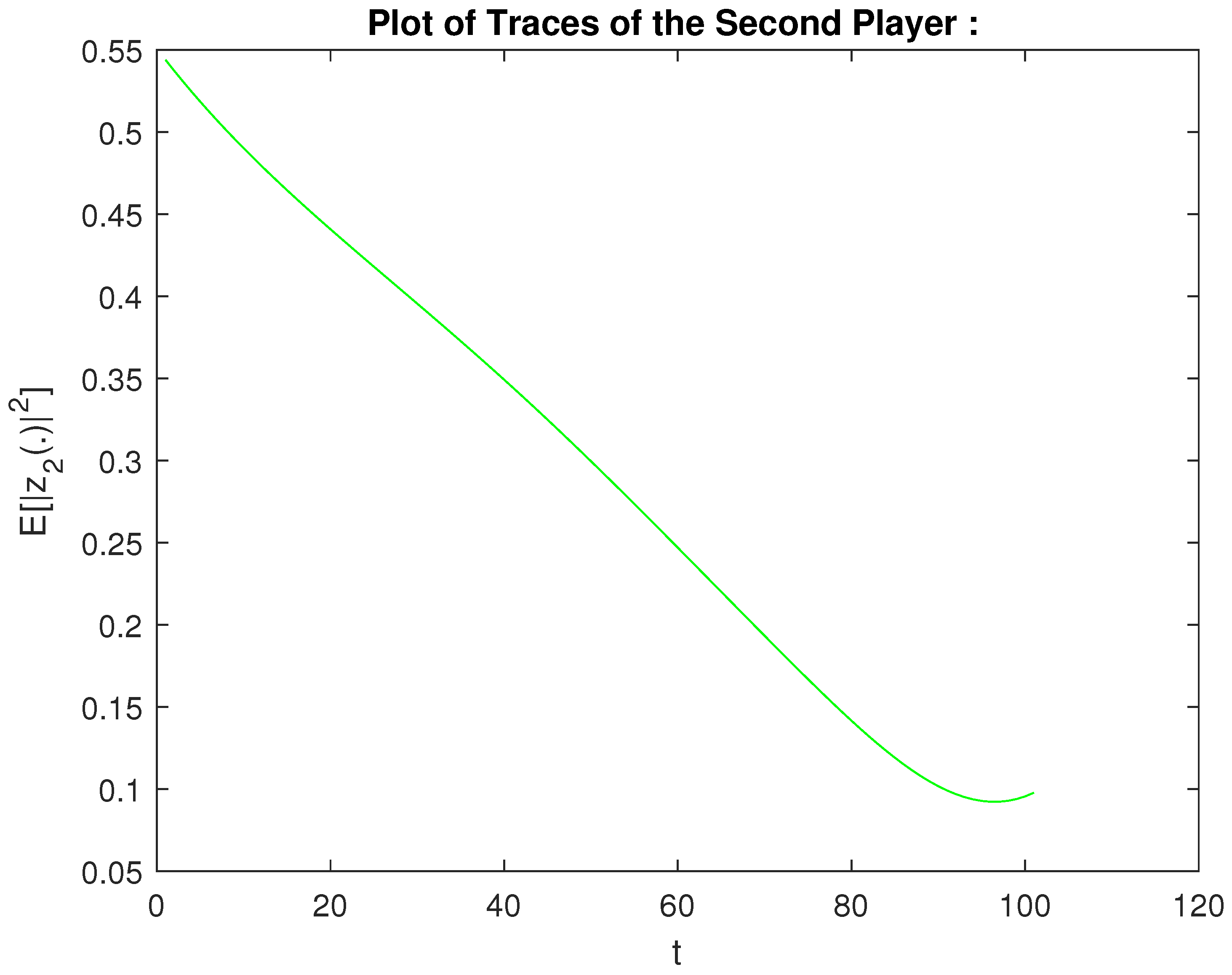
(A).

The base variant using the above matrix coefficients. We have executed Step 1 and Step 2. The computed values $\mathbb{E}\left[\right|{\tilde{z}}_k\left(jh\right){|}^2],k=1,2$ for the signals ${\tilde{z}}_k,k=1,2$ of the players are given on Figure 1 and Figure 2 for the first player and the second player, respectively. Moreover, we have obtained the following values of $E\left[\right|z_k\left(1\right)-{\zeta }_k{|}^2]$ for the players $k=1,2$ , i.e.,

$$E\left[\right|z_1\left(1\right)-{\zeta }_1{|}^2]=0.5033,E[|z_2\left(1\right)-{\zeta }_2{|}^2]=1.0173.$$

(39)

Figure 1. Plot of traces of the first player: $\mathbb{E}\left[\right|{\tilde{z}}_1\left(jh\right){|}^2]\mathrm{in}[0,t_f]=[0,1]$.

Figure 2. Plot of traces of the second player: $\mathbb{E}\left[\right|{\tilde{z}}_2\left(jh\right){|}^2]\mathrm{in}[0,t_f]=[0,1]$.

(B).

We want to compute the output of the closed-loop system $z_k(·)$ by using a control law (other than the optimal one) ${\tilde{u}}_k\left(jh\right)=F_k\left(jh\right)x\left(jh\right)+{\phi }_k\left(jh\right)$ with $k=1,2,j=0,1,\dots ,N-1$. For this, we take $F_k\left(jh\right)$ and ${\phi }_k\left(jh\right)$ different from the optimal cases. We use the same matrix coefficients. After Step 1, we obtain the optimal values of ${\tilde{F}}_k\left(jh\right)$ and ${\tilde{\phi }}_k\left(jh\right)k=1,2$. Then, we compute the different values ${\tilde{F}}_k^k\left(jh\right),{\tilde{\phi }}_k^k\left(jh\right),k=1,2$ as follows ($j=0,1,\dots ,N-1$):

$${\tilde{F}}_1^1\left(jh\right)=({\tilde{F}}_1\left(jh\right)+{\tilde{F}}_2\left(jh\right))/2,{\tilde{F}}_2^2\left(jh\right)=({\tilde{F}}_1\left(jh\right)-{\tilde{F}}_2\left(jh\right))/2,$$

$${\tilde{\phi }}_1^1\left(jh\right)=({\tilde{\phi }}_1\left(jh\right)-{\tilde{\phi }}_2\left(jh\right))/2,{\tilde{\phi }}_2^2\left(jh\right)=({\tilde{\phi }}_1\left(jh\right)+{\tilde{\phi }}_2\left(jh\right))/2.$$

The computations continue with Step 2 with ${\tilde{F}}_k^k\left(jh\right),{\tilde{\phi }}_k^k\left(jh\right),k=1,2$. The computed values of $E\left[\right|z_k\left(1\right)-{\zeta }_k{|}^2],k=1,2$ are

$$E\left[\right|z_1\left(1\right)-{\zeta }_1{|}^2]=8.5203,E[|z_2\left(1\right)-{\zeta }_2{|}^2]=4.5174.$$

(40)

One sees from (39) and (40) that the values of the obtained deviation from the target provided by the optimal control are better than the ones provided by another control.

6. Conclusions

In this work, we studied the problem of the minimization of the deviation of some outputs of a controlled dynamical system from some given reference signals. We considered the case where the dynamical system is controlled by two decision-makers which are not cooperating. One of the two decision-makers wants to minimize the deviation of a preferential output of the dynamical system from a given reference signal, whereas the other decision-maker wants to minimize the deviation of another output of the same dynamical controlled system from another reference signal. This problem was viewed as a problem of designing a Nash equilibrium strategy for an affine quadratic differential game with two players. Since it was supposed that the controlled dynamical system is subject to multiplicative white noise perturbations and Markovian jumping, we must find a Nash equilibrium strategy for a stochastic affine quadratic differential game. We have obtained explicit formulae of the equilibrium strategy. To this end, the solutions of two TVPs were involved. The first TVP is associated with a hybrid system formed by two nonlinear backward differential equations and two nonlinear algebraic equations, namely, the TVP (30). The second TVP is associated with a hybrid system formed by two backward linear differential equations coupled with two affine matrix algebraic equations, that is TVP (31). The first TVP is the same as that involved in the description of the Nash equilibrium strategy for an LQ differential game. The second TVP takes into consideration the reference signals $r_k(·)$ together with the final targets ${\zeta }_k,k=1,2$.

There are few directions that can be considered as future research:

• Direct extensions from this article can be considered as follows: the case when two or more players (with different cost functionals) are willing to cooperate or the case when $t_f\to \infty$ for the tracking problem associated with a controlled system of type (1).
• Anther direction of future research can consider the case of a tracking problem with preview in the case when the controlled dynamical system is affected by state multiplicative and/or control multiplicative white noise perturbations. To our knowledge, this case was not yet considered in the existing literature. Some results in this direction have been reported, for example in [2,6,7], for the case of only one decision-maker and [29,30] for the case with more than one decision-maker.
• Finally, other directions can consider the case of linear quadratic tracking problem with a delay component (for one or more players) for Itô stochastic systems. Some results in this direction have been reported for examples in [10,11].

References

- Axelband, E. The structure of the optimal tracking problem for distributed-parameter systems. IEEE Trans. Autom. Control 1968, 13, 50–56. [Google Scholar] [CrossRef]
- Cohen, A.; Shaked, U. Linear discrete-time H∞-optimal tracking with preview. IEEE Trans. Autom. Control 1997, 42, 270–276. [Google Scholar] [CrossRef]
- Emami-Naeini, A.; Franklin, G. Deadbeat control and tracking of discrete-time systems. IEEE Trans. Autom. Control 1982, 27, 176–181. [Google Scholar] [CrossRef]
- Liu, D.; Liu, X. Optimal and minimum-energy optimal tracking of discrete linear time-varying systems. Automatica 1995, 31, 1407–1419. [Google Scholar] [CrossRef]
- Shaked, U.; de Souza, C.E. Continuous-time tracking problems in an H∞ setting: A game theory approach. IEEE Trans. Autom. Control 1995, 40, 841–852. [Google Scholar] [CrossRef]
- Gershon, E.; Shaked, U.; Yaesh, I. H∞ tracking of linear systems with stochastic uncertainties and preview. IFAC Proc. Vol. 2002, 35, 407–412. [Google Scholar] [CrossRef]
- Gershon, E.; Limebeer, D.J.N.; Shaked, U.; Yaesh, I. Stochastic H∞ tracking with preview for state-multiplicative systems. IEEE Trans. Autom. Control 2004, 49, 2061–2068. [Google Scholar] [CrossRef]
- Dragan, V.; Morozan, T. Discrete-time Riccati type equations and the tracking problem. ICIC Express Lett. 2008, 2, 109–116. [Google Scholar]
- Dragan, V.; Morozan, T.; Stoica, A.M. Mathematical Methods in Robust Control of Linear Stochastic Systems; Springer: New York, NY, USA, 2013. [Google Scholar]
- Han, C.; Wang, W. Optimal LQ tracking control for continuous-time systems with pointwise time-varying input delay. Int. J. Control. Autom. Syst. 2017, 15, 2243–2252. [Google Scholar] [CrossRef]
- Jin, N.; Liu, S.; Zhang, H. Tracking Problem for Itô Stochastic System with Input Delay. In Proceedings of the Chinese Control Conference (CCC), Guangzhou, China, 27–30 July 2019; pp. 1370–1374. [Google Scholar]
- Pindyck, R. An application of the linear quadratic tracking problem to economic stabilization policy. IEEE Trans. Autom. Control 1972, 17, 287–300. [Google Scholar] [CrossRef]
- Alba-Florest, R.; Barbieri, E. Real-time infinite horizon linear quadratic tracking controller for vibration quenching in flexible beams. In Proceedings of the IEEE International Conference on Systems, Man and Cybernetics, Taipei, Taiwa, 8–11 October 2006; pp. 38–43. [Google Scholar]
- Wang, Y.-L.; Yang, G.-H. Robust H∞ model reference tracking control for networked control systems with communication constraints. Int. J. Control. Autom. Syst. 2009, 7, 992–1000. [Google Scholar] [CrossRef]
- Ou, M.; Li, S.; Wang, C. Finite-time tracking control for multiple non-holonomic mobile robots based on visual servoing. Int. J. Control 2013, 86, 2175–2188. [Google Scholar] [CrossRef]
- Fu, Y.-M.; Lu, Y.; Zhang, T.; Zhang, M.-R.; Li, C.-J. Trajectory tracking problem for Markov jump systems with Itô stochastic disturbance and its application in orbit manoeuvring. IMA J. Math. Control. Inf. 2018, 35, 1201–1216. [Google Scholar] [CrossRef]
- Basar, T. Nash equilibria of risk-sensitive nonlinear stochastic differential games. J. Optim. Theory Appliations 1999, 100, 479–498. [Google Scholar] [CrossRef]
- Buckdahn, R.; Cardaliaguet, P.; Rainer, C. Nash equilibrium payoffs for nonzero-sum stochastic differential games. SIAM J. Control. Optim. 2004, 43, 624–642. [Google Scholar] [CrossRef]
- Sun, H.Y.; Li, M.; Zhang, W.H. Linear quadratic stochastic differential game: Infinite time case. ICIC Express Lett. 2010, 5, 1449–1454. [Google Scholar]
- Sun, H.; Yan, L.; Li, L. Linear quadratic stochastic differential games with Markov jumps and multiplicative noise: Infinite time case. Int. J. Innov. Comput. Inf. Control 2015, 11, 348–361. [Google Scholar]
- Nakura, G. Nash tracking game with preview by stare feedback for linear continuous-time systems. In Proceedings of the 50th ISCIE International Symposium on Stochastic Systems Theory and Its Applications, Kyoto, Japan, 1–2 November 2018; pp. 49–55. [Google Scholar]
- Fridman, A. Stochastic Differential Equations and Applications; Academic: New York, NY, USA, 1975; Volume I. [Google Scholar]
- Oksendal, B. Stoch. Differ. Equations; Springer: Berlin/Heidelberg, Germany, 2003. [Google Scholar]
- Chung, K.L. Markov Chains with Stationary Transition Probabilities; Springer: Berlin/Heidelberg, Germany, 1967. [Google Scholar]
- Doob, J.L. Stochastic Processes; Wiley: New York, NY, USA, 1967. [Google Scholar]
- Boukas, E.R. Stochastic Switching Systems: Analysis and Design; Birkhäuser: Boston, MA, USA, 2005. [Google Scholar]
- Costa, O.L.V.; Fragoso, M.D.; Marques, R.P. Discrete-Time Markov Jump Linear Systems; Series: Probability and Its Applications; Springer: London, UK, 2005. [Google Scholar]
- Costa, O.L.V.; Fragoso, M.D.; Todorov, M.G. Continuous-Time Markov Jump Linear Systems; Series: Probability and Its Applications; Springer: Berlin/Heidelberg, Germany, 2013. [Google Scholar]
- Nakura, G. Soft-Constrained Nash Tracking Game with Preview by State Feedback for Linear Continuous-Time Markovian Jump Systems. In Proceedings of the 2018 57th Annual Conference of the Society of Instrument and Control Engineers of Japan (SICE), Nara, Japan, 11–14 September 2018; pp. 450–455. [Google Scholar]
- Nakura, G. Nash Tracking Game with Preview by State Feedback for Linear Continuous-Time Markovian Jump Systems. In Proceedings of the 50th ISCIE International Symposium on Stochastic Systems Theory and Its Applications, Kyoto, Japan, 1–2 November 2018; pp. 56–63. [Google Scholar]
Disclaimer/Publisher’s Note: The statements, opinions and data contained in all publications are solely those of the individual author(s) and contributor(s) and not of MDPI and/or the editor(s). MDPI and/or the editor(s) disclaim responsibility for any injury to people or property resulting from any ideas, methods, instructions or products referred to in the content. |
© 2023 by the authors. Licensee MDPI, Basel, Switzerland. This article is an open access article distributed under the terms and conditions of the Creative Commons Attribution (CC BY) license (https://creativecommons.org/licenses/by/4.0/).
Share and Cite
Drăgan, V.; Ivanov, I.G.; Popa, I.-L. A Game—Theoretic Model for a Stochastic Linear Quadratic Tracking Problem. Axioms 2023, 12, 76. https://doi.org/10.3390/axioms12010076
Drăgan V, Ivanov IG, Popa I-L. A Game—Theoretic Model for a Stochastic Linear Quadratic Tracking Problem. Axioms. 2023; 12(1):76. https://doi.org/10.3390/axioms12010076
Chicago/Turabian StyleDrăgan, Vasile, Ivan Ganchev Ivanov, and Ioan-Lucian Popa. 2023. "A Game—Theoretic Model for a Stochastic Linear Quadratic Tracking Problem" Axioms 12, no. 1: 76. https://doi.org/10.3390/axioms12010076
APA StyleDrăgan, V., Ivanov, I. G., & Popa, I.-L. (2023). A Game—Theoretic Model for a Stochastic Linear Quadratic Tracking Problem. Axioms, 12(1), 76. https://doi.org/10.3390/axioms12010076