Article

Digital Coupon Promotion and Inventory Strategies of Omnichannel Brands

School of Management, Hefei University of Technology, Hefei 230009, China
*
Author to whom correspondence should be addressed.
Axioms 2023, 12(1), 29; https://doi.org/10.3390/axioms12010029
Submission received: 29 October 2022 / Revised: 1 December 2022 / Accepted: 21 December 2022 / Published: 26 December 2022
(This article belongs to the Special Issue Applied Mathematics, Intelligence and Operations Research)

Abstract

:
This paper investigates when an omnichannel brand should offer digital coupons in the online and buy-online-and-pick-up-in-store (BOPS) channels and, if so, the joint decision of coupon face value and store inventory. The impact of a digital coupon promotion on store inventory is also explored. Two scenarios are considered, one where consumers’ costs in the online and store channels are homogeneous and another in which they are heterogeneous, and two newsvendor models, with and without a coupon promotion, are constructed under each scenario. The results show that the issuance of coupons improves the omnichannel brand’s profit when the price is high and the coefficient of the difference in valuation between two types of consumers is low in the homogeneous scenario. In the heterogeneous scenario, the brand prefers the coupon promotion when the price is high or moderate and the coefficient of the difference in valuation between two types of consumers is high. In addition, offering a coupon promotion yields a higher store inventory in most cases. However, store inventory is decreased in some special cases in the homogeneous scenario. Moreover, an increased hassle cost in the BOPS channel significantly lowers the offline demand and profit increase from a digital coupon promotion. Furthermore, a coupon promotion is more likely to benefit both the brand and consumers as the cross-selling revenue increases. These results provide guidance for omnichannel brands to implement coupon promotions and adjust store inventory with stochastic demand.

1. Introduction

1.1. Background and Problem Description

With the rapid development of omnichannel retailing, the BOPS (buy-online-and- pick-up-in-store) strategy is becoming increasingly popular. During the COVID-19 pandemic, approximately two-thirds of US customers shopped online, and BOPS saw more than 500% growth [1]. Kim et al. [2] reported that BOPS benefits both firms and consumers. It reduces the waiting time of consumers after placing an order online and gives them the opportunity to experience the product. In addition, it improves store traffic and sales since BOPS customers tend to make additional purchases in store [3]. Additionally, BOPS enables firms to reach new customers by providing real-time information about inventory availability and by reducing the hassle cost of shopping [4]. Therefore, an increasing number of brands have provided BOPS (buy-online-and-pick-up-in-store) services to integrate the advantages of online and store channels. For example, Apple provides consumers with more choices and flexibility through BOPS (such as product availability and store delivery). UNIQLO, a Japanese clothing brand, implemented BOPS in 2016, and the BOPS channel increased sales significantly [5].
The distribution of coupons is an effective tool for firms to implement price discrimination and capture new consumers to enhance profitability [6]. Due to fierce market competition, an increasing number of firms have recognized the importance of price promotion tools such as coupons, rebates and group buying [7]. Coupons are the most popular and widely used of these tools because of their low cost and convenience. Moreover, the growth in internet adoption has made digital coupons a popular promotional tool [8]. Although price discrimination is illegal in some countries, it is very common for firms to adopt price discrimination by using digital coupons around the world because some consumers are unwilling to register to obtain coupons due to concerns about information security or they are too busy or forget to redeem coupons before the expiration date [9]. For example, Apple and UNIQLO use digital coupons to stimulate demand. Data from Kantar show that 3282 brands provided nearly $8.7 billion in e-coupon incentives in 2021 [10]. In addition, brands often distribute digital coupons in the online and BOPS channels to capture more market share in an omnichannel setting [11,12]. In practice, omnichannel brands usually adopt a unified pricing strategy for all channels to create synergy [13]. Therefore, the difference in the coupon strategies of brands across channels makes consumers’ actual payments diverse among channels. This affects consumers’ channel choices, leads to their channel transfer behaviors, and ultimately influences brands’ profits [14]. Furthermore, coupon promotions lower brands’ marginal profits. If the coupon face values are too large, the brands’ marginal profits are low. If the coupon face values are too small, the sales volume of products does not increase significantly. Therefore, considering the competition, potential erosion of market share, and profit between channels in an omnichannel environment [11], deciding whether to offer a digital coupon promotion is an important and challenging problem faced by each brand.
In an environment of uncertain demand, reasonable inventory decision-making is another essential way for brands to boost profits and market competitiveness [15]. Gao and Su [16], Yang et al. [17], Jiu [18], and Hu et al. [19] studied inventory decisions under omnichannel fulfillment strategies, such as BOPS, showroom, ship-from-store, BORS (buy-online-and-return-in-store), and inventory-pooling policies. However, they neglected the impact of price promotions, such as coupons, on inventory decisions. Obviously, digital coupons enhance consumers’ purchase intentions and thus increase demand [20]. With the widespread use of digital coupons, many brands attempt to quantify the impact of coupons on operational strategies, especially inventory management. In an omnichannel environment, coupon promotions complicate inventory decisions. On the one hand, the provision of inventory availability information with the introduction of BOPS leads to the influence of store inventory on consumers’ purchasing decisions. In this situation, low store inventory is likely to cause brands to lose some demand due to stockouts [21], while high store inventory increases brands’ inventory costs. This means that the inventory decisions of brands implementing BOPS are important and differ from those in the traditional dual-channel environment. On the other hand, for omnichannel brands, coupons induce consumers to switch channels, thus affecting the demand of each channel and store inventory. Therefore, decisions regarding digital coupon promotions and inventory have become more challenging, and omnichannel brands urgently need to solve the following problems: under what conditions should digital coupons be issued through the online and BOPS channels for promotions? How can a joint decision be made on coupon face value and store inventory if the brand opts to offer a promotion? If there is no promotion, how should store inventory be determined? How does a digital coupon promotion affect store inventory? Surprisingly, to date, no research has been conducted on these issues. It is vital for brands to learn how to enhance profitability through well-designed coupon–inventory combination strategies.
To address these questions, we develop a newsboy model in which a brand that operates online, BOPS and store channels offers digital coupons to attract potential customers in the online and BOPS channels. Customers strategically choose which channel to patronize to maximize individual utility. We first analyze the scenario where consumers’ hassle costs in the online and store channels are homogeneous. We study a joint decision regarding coupon face value and store inventory under a coupon promotion and examine the impact of the coupon promotion on total profits. Using these results, we determine whether digital coupons should be issued and how a coupon promotion affects store inventory. Then, we consider a more general situation with heterogeneous online and offline hassle costs for consumers.

1.2. Contributions and Findings

Our research makes the following contributions. First, to the best of our knowledge, this study is amongst the first to examine an omnichannel brand’s digital coupon promotion and inventory strategies considering coupons’ role in price discrimination and market expansion, while previous literature has not yet identified the interaction between coupon policy and inventory management in omnichannel retailing. It is a combination of marketing and operation. Second, we provide theoretical foundations and business guidance for an omnichannel brand regarding whether it should offer digital coupons and to help it make the best inventory and coupon face value decisions if it does so. Because promotions are often more flexible than pricing, China’s government has enacted regulations prohibiting merchants from changing the original price during a promotion. Therefore, our guidance will be useful for brands to improve their profits and market competitiveness. Third, we investigate the effect of coupon promotions on demand, inventory, and profits from the perspective of the hassle cost in the BOPS channel. A higher hassle cost in the BOPS channel weakens the offline demand expansion and profit enhancement effects of digital coupons, which enriches the literature on coupon promotion.
Our first main finding is that the distribution of digital coupons in the online and BOPS channels may not be profitable. Specifically, in the homogeneous scenario, it is optimal for the brand to engage in coupon promotion only when the price is high and the coefficient of the difference in valuation between two types of consumers is low. Similarly, in the heterogeneous scenario, the brand should promote when the price is high or when the price is moderate but the coefficient of the difference in valuation is high. Second, a coupon promotion reduces store inventory if the proportion of H-type consumers is high, the unit inventory cost is not too high, and the price is high in the homogeneous scenario, but it always increases store inventory in the heterogeneous scenario. Third, the hassle cost in the BOPS channel negatively influences the promotional effect of digital coupons. Finally, when coupons are issued, higher cross-selling revenue contributes to higher profit, store inventory, and coupon face value, which benefits both consumers and the brand.
The remainder of the paper is organized as follows: Section 2 reviews the relevant literature. Section 3 describes the model and derives the optimal decisions. In Section 4, we conduct numerical experiments to assess the impacts of the model parameters on the brand’s optimal policies and to derive some managerial implications. Finally, we conclude the paper and present directions for further research in Section 5. The proofs of all propositions are provided in Appendix A.

2. Literature Review

2.1. Joint Pricing and Inventory Decisions

Because we assume that the price is exogenous and that the price actually paid by consumers is affected by coupons, joint pricing and inventory decisions are closely related to this study. Since Whitin [22] pioneered the problem, many studies have considered deterministic demand [23,24,25]. Other researchers have investigated the problem under stochastic demand considering supply uncertainty [26,27], reference price effect [28,29], perishable items [15,30] and loss aversion [31]. In recent years, an increasing number of scholars have extended this research stream by involving price discounts [32,33] or omnichannel retailing [34,35], which are most relevant to our work. For example, Zhang et al. [36] developed a two-stage model to reveal why and how brands use flash sales to sell a limited number of new products at discounted prices within a finite time and in single-channel settings. Gupta et al. [34] considered an omnichannel situation where the retailer used either the distribution center or any of its offline stores to fulfill online orders. Zhang et al. [37] derived optimal pricing and inventory decisions considering the ROPS (online-pick-up-and-pay-in-store) mode. Qiu et al. [35] proposed a robust omnichannel pricing and ordering optimization model with different return policies. However, these studies focus on pricing decisions or a single-channel context. None of them combines the impact of consumers’ choices among multiple channels on store inventory decisions with price promotions. We endeavor to address this research gap by characterizing the price discrimination function of coupons and exploring the joint coupon promotion and inventory strategy when BOPS is implemented.

2.2. Coupon Promotions

There are three lines of research on coupon promotions. The first concerns coupon redemption. For example, Noble et al. [38] reported that after accounting for shopping cart size, lower-income consumers redeemed coupons at higher rates than most of the higher-income categories. Ren et al. [39] applied a clustering algorithm to forecast consumers’ purchase intention with e-coupons. Ladhari et al. [40] investigated the determinants and consequences of redemption for geo-targeted mobile coupons. Nayal and Pandey [41] developed a reliable and valid scale for measuring digital coupon redemption with the grounded theory approach. The second line investigates the marketing effect of coupons for a firm. For instance, Lu and Moorthy [42] found that rebates were more efficient in surplus extraction but coupons offered more control over whom to serve. Gabel and Guhl [43] compared the effectiveness of rewards and individually-targeted coupons in loyalty programs. Duan et al. [44] empirically studied how online reviews and coupons affected sales, pricing, and profit. The third line involves coupon promotion in the supply chain [6,45,46]. For example, Su et al. [6] claimed that coupon trading cannot simultaneously benefit retailers and manufacturers. Bauner et al. [47] noted that the positioning of a private-label product in terms of quality and feature differentiation from a national brand played an important role in the profits of manufacturers and retailers. The recent papers most related to our research are Jiang et al. [48], Li et al. [11], Li et al. [12], and Li et al. [49]. The first three papers explored coupon strategies for an omnichannel retailer. Li et al. [49] studied the optimal price and coupon promotion strategies in an omnichannel supply chain where the manufacturer sells competitive products via the BOPS channel and the retailer’s offline channel. However, they focused on coupon strategies and did not consider the interaction between coupon promotion and inventory, whereas we combine omnichannel coupon promotion with inventory management and investigate the optimal coupon face value and inventory level for an omnichannel brand. Exploring the influence of coupons across multiple channels on store inventory is significant, considering their increasing prevalence.

2.3. Omnichannel Retailing

Omnichannel retailing has received considerable attention. A large body of literature has focused on omnichannel fulfillment strategies, such as BOPS [17,50], showroom [16,51], ship-from-store [18,52], and BORS [53,54]. For example, Jin et al. [50] proposed a strategy for determining the BOPS service area and provided a retailer with guidelines for judging the product type for in-store pickup. Zhong et al. [51] found that a certain level of showrooming may be beneficial for brick-and-mortar stores but that webrooming always harms online retailers. Yang and Ji [54] considered three mechanisms associated with managing consumer returns for an omnichannel retailer: BORS, return insurance and a virtual try-on experience. There are other topics in omnichannel retailing, such as customer experience [55,56], channel integration [3,52], and handling of demand uncertainty [57]. Although issues related to omnichannel retailing, particularly channel pricing strategies, have been widely explored, the existing works mainly focus on the conditions for adopting omnichannel fulfillment options, and research on coupon promotion and inventory control is scarce. We contribute to the literature by examining coupon promotion and inventory strategies for a brand with a BOPS channel, and our findings can provide valuable insights into omnichannel settings.
In summary, this paper differs from previous studies in the following two aspects. First, to the best of our knowledge, we are almost the first to study the joint digital coupon promotion and inventory strategies when an omnichannel brand provides BOPS service by using the newsvendor approach. Second, we consider the price-discriminatory role of e-coupons by dividing consumers into two categories based on their valuation, and construct consumers’ utility functions when purchasing in three channels to describe the impact of digital coupons on consumers’ channel choices and the corresponding store inventory.

3. Model

There is a brand that sells a product through online, store and BOPS channels at exogenous price p . The brand faces a newsvendor problem, that is, the brand needs to determine the store inventory level q before random demand is realized. c is the unit cost of inventory, and the salvage value of leftover units is normalized to zero. Because this paper focuses on coupon promotion and inventory decisions rather than the BOPS strategy, the production cost and sales cost are also normalized to zero. In addition, each consumer brings the cross-selling revenue r to the brand since consumers often make additional purchases when they come to a store [37,58]. In line with Gao and Su [16], the online channel is modeled exogenously. Therefore, the brand simply obtains a net profit margin p from each unit of online demand. In practice, UNIQLO’s online shopping website directly displays the status of store inventory while providing a BOPS option. When the store is out of stock, the BOPS option is unavailable. Moreover, numerous customers verify inventory availability online without actually using the BOPS functionality because this information is immediately accessible online, and the cost is negligible compared with the sunk cost of traveling to the store but encountering a stockout. In this special case, Gallino and Moreno [3] identified that online sales may decrease, while store sales may increase after the adoption of BOPS. Therefore, it is reasonable to assume that the implementation of BOPS enables consumers to know the store inventory status before they visit the store [4]. The demand of consumers who prefer purchasing through the BOPS or store channel but encounter stockouts in the store can be met if they obtain nonnegative utilities of online purchase and therefore shift online. Additionally, the market demand D is random and follows a continuous distribution F and density f . Customers choose among the online, store and BOPS channels to maximize their utilities.
Our model differs from the classic newsvendor model in two areas. First, in an omnichannel environment, consumers’ channel choices affect the brand’s inventory decision. In a particular case where all consumers prefer to buy online, the brand does not need to stock the product offline and does not face a newsboy problem. Second, we incorporate the channel transfer behavior of consumers who tend to come to the store but eventually purchase online due to shortages of the product in the store into our model. Specifically, the omnichannel brand’s profit function includes the profits of multiple channels and may contain the profit from consumers who transfer to the online market, which is different from the profit function of a traditional newsboy.
Following previous studies [9,59], we divide consumers into two types according to their valuation: H-type consumers (high-value/price-insensitive consumers) and L-type consumers (low-value/price-sensitive consumers). An H-type consumer’s valuation of the brand’s product is v , while an L-type consumer’s valuation is lower and given by δ v , where δ is the valuation coefficient of L-type consumers for products relative to H-type consumers and δ ( 0 , 1 ) . Then, we define 1 δ as the coefficient of the difference in valuation between two types of consumers. The larger δ is, the smaller 1 δ is, and the smaller the valuation difference between the two types of consumers is. We assume that the proportions of H-type and L-type consumers are λ and 1 λ , respectively, where λ ( 0 , 1 ) . Furthermore, we assume that H-type consumers never buy promotional products because they are usually high-income groups and value time sufficiently that they are unwilling to pay the opportunity cost of searching for or using coupons. Namely, the redemption cost is prohibitively high for H-type consumers [42]. This assumption is widely adopted in the marketing and economics literature on coupon promotions [9,60]. In contrast, the redemption cost of L-type consumers is normalized to zero; hence, they always use coupons when available [47]. Moreover, each customer incurs hassle costs h o , h s , and h b when shopping in the online, store and BOPS channels, respectively. Table 1 summarizes the symbols used in the paper. Then, we consider the homogeneity and heterogeneity of h o and h s in Section 3.1 and Section 3.2, respectively.

3.1. Homogeneous Online and Store Hassle Costs

In this section, we consider the scenario where consumers’ costs in the online and store channels are homogeneous. Because there are two types of consumers with different valuations in the market, the brand has two price strategies: a low-price strategy and a high-price strategy. In the former, a low price is formulated to encourage both types of consumers to buy, and in the latter, a price so high that only H-type consumers make purchases is used. Under the low-price strategy, the brand has no incentive to conduct coupon promotions since the market is fully covered. Therefore, only under the high-price strategy will the brand do so. Since H-type consumers will not use coupons to buy products, enterprises can encourage L-type consumers to buy while still gaining a high margin from H-type consumers by issuing coupons under the high-price strategy. Accordingly, when the price is high (only H-type consumers purchase when there is no coupon promotion), the brand initiates a coupon promotion.
Next, we explore the joint decision of coupon face value and store inventory when the brand holds a coupon promotion. The brand offers digital coupons in the online and BOPS channels for market expansion with the same coupon face value f . Note that only L-type consumers use coupons, and the utility of an L-type consumer purchasing in the online, BOPS, and store channels is u o L = δ v p + f h o , u b L = δ v p + f h b and u s L = δ v p + f h s , respectively. However, the utility of an H-type consumer purchasing through the online, BOPS and store channels is u o H = v p h o , u b H = v p h b and u s H = v p h s , respectively. When h o is the lowest hassle cost, consumers never go to the store, and the brand issues coupons to induce all consumers to buy online. The brand will stock nothing in the store (i.e., q * = 0 ) and earn an expected profit π * = p E D . When h o exceeds either h b or h s , the brand will issue coupons to encourage L-type consumers to purchase through the online or BOPS channel. H-type consumers buy in the BOPS or store channel. When consumers encounter store shortages, H-type consumers decide whether to switch to purchasing online based on the price and online hassle cost, while L-type consumers’ decisions regarding whether to switch to online also depend on the coupon face value. Then, we can obtain the brand’s expected profit in different consumer transfer situations. In line with Su [61] and He et al. [62], we can derive the brand’s optimal coupon promotion and store inventory strategies by maximizing its profit, namely Proposition 1. We use q * and f * to represent the optimal store inventory level and the optimal coupon face value when the brand conducts a coupon promotion. q B * denotes the optimal store inventory level when there is no coupon promotion.
Proposition 1. 
The optimal strategy of the brand is as follows:
(1) 
When  h o < min ( h b , h s ) and p = δ v h o , the brand does not offer coupons, then q B * = 0 .
(2) 
When h b < min ( h o , h s ) , p = δ v h b and v > h o h b 1 δ , the brand does not offer coupons, and if c < ( 1 λ ) ( δ v h b ) + r , then q B * = F ¯ 1 ( c ( 1 λ ) ( δ v h b ) + r ) ; otherwise, q B * = 0 . When h b < min ( h o , h s ) , p = δ v h b and v h o h b 1 δ , the brand does not offer coupons, and if c < δ v h b + r , then q B * = F ¯ 1 ( c δ v h b + r ) ; otherwise, q B * = 0 . When h b < min ( h o , h s ) and p = δ v h o , the brand does not offer coupons, and if c < r , q B * = F ¯ 1 ( c r ) ; otherwise, q B * = 0 .
(3) 
When h s < min ( h o , h b ) , p = δ v h s and v > h o h s 1 δ , the brand does not offer coupons, and if c < ( 1 λ ) ( δ v h s ) + r , then q B * = F ¯ 1 ( c ( 1 λ ) ( δ v h s ) + r ) ; otherwise, q B * = 0 . When h s < min ( h o , h b ) , p = δ v h s and v h o h s 1 δ , the brand does not offer coupons, and if c < δ v h s + r , then q B * = F ¯ 1 ( c δ v h s + r ) ; otherwise, q B * = 0 . When h s < min ( h o , h b ) and p = δ v h o , the brand does not offer coupons, and if c < r , then q B * = F ¯ 1 ( c r ) ; otherwise, q B * = 0 .
(4) 
When h o < min ( h b , h s ) and p = v h o , if h o < δ v , then f * = ( 1 δ ) v and q * = 0 .
(5) 
When h b < min ( h o , h s ) and p = v h b , if h o < δ v , c < λ ( v h b ) + r and λ > λ 1 , or h o < δ v and λ ( v h b ) + r c < λ v + ( 1 λ ) δ v + r h b , or h b < δ v < h o and c < λ v + ( 1 λ ) δ v + r h b , then f * = ( 1 δ ) v and q * = F ¯ 1 ( c λ v + ( 1 λ ) δ v + r h b ) . If h o < δ v , c < λ ( v h b ) + r and λ λ 1 , then f * = ( 1 δ ) v + h o h b and q * = F ¯ 1 ( c λ ( v h b ) + r ) . If h b < δ v and λ v + ( 1 λ ) δ v + r h b c < v h b + r , or h b δ v and c < v h b + r , the brand does not offer coupons, then q B * = λ F ¯ 1 ( c v + r h b ) . If c v h b + r and h o < δ v , then f * = ( 1 δ ) v + h o h b and q * = 0 .
(6) 
When h b < min ( h o , h s ) , p = v h o and v > h o h b 1 δ , or h s < h b < h o , p = v h o and v > h o h s 1 δ , if h o < δ v , c < r and λ > λ 2 , or h o < δ v and r c < ( 1 λ ) ( δ v h b ) + r , or h b < δ v < h o and c < ( 1 λ ) ( δ v h b ) + r , then f * = ( 1 δ ) v + h b h o and q * = F ¯ 1 ( c ( 1 λ ) ( δ v h b ) + r ) . If h o < δ v , c < r and λ λ 2 , then f * = ( 1 δ ) v and q * = F ¯ 1 ( c r ) . If h b δ v and c < r , the brand does not offer coupons, then q B * = λ F ¯ 1 ( c r ) . If h o < δ v and c ( 1 λ ) ( δ v h b ) + r , then f * = ( 1 δ ) v and q * = 0 . If h b < δ v < h o and c ( 1 λ ) ( δ v h b ) + r , or h b δ v and c r , the brand does not offer coupons, then q B * = 0 .
(7) 
When h s < h o < h b and p = v h s , if h o < δ v and c < v h s + r , then f * = ( 1 δ ) v + h o h s and q * = λ F ¯ 1 ( c v h s + r ) . If h o < δ v and c v h s + r , then f * = ( 1 δ ) v + h o h s and q * = 0 . If h o δ v and c < v h s + r , the brand does not offer coupons, then q B * = λ F ¯ 1 ( c v h s + r ) . When h s < h b < h o and p = v h s , if h o < δ v , c < λ ( v h s ) + r and λ > λ 3 , or h o < δ v and λ ( v h s ) + r c < λ v + ( 1 λ ) δ v + r λ h s ( 1 λ ) h b , or h b < δ v < h o and c < λ v + ( 1 λ ) δ v + r λ h s ( 1 λ ) h b , then f * = ( 1 δ ) v + h b h s and q * = F ¯ 1 ( c λ v + ( 1 λ ) δ v + r λ h s ( 1 λ ) h b ) . If h o < δ v , c < λ ( v h s ) + r and λ λ 3 , then f * = ( 1 δ ) v + h o h s and q * = F ¯ 1 ( c λ ( v h s ) + r ) . If h b < δ v and λ v + ( 1 λ ) δ v + r λ h s ( 1 λ ) h b c < v h s + r , or h b δ v and c < v h s + r , the brand does not offer coupons, then q B * = λ F ¯ 1 ( c v + r h s ) . If c v h s + r and h o < δ v , then f * = ( 1 δ ) v + h o h s and q * = 0 .
(8) 
When h s < h o < h b , p = v h o and v > h o h s 1 δ , if h o < δ v and c < r , then f * = ( 1 δ ) v and q * = λ F ¯ 1 ( c r ) . If h o < δ v and c r , then f * = ( 1 δ ) v and q * = 0 . If h o δ v and c < r , the brand does not offer coupons, then q B * = λ F ¯ 1 ( c r ) . If h o δ v and c r , the brand does not offer coupons, then q B * = 0 . λ 1 , λ 2 and λ 3 are constants defined in theAppendix A.
Proposition 1 demonstrates that in the scenario where the online and store hassle costs of consumers are homogeneous, the brand issues digital coupons in the online and BOPS channels when the product price p is high and the coefficient of the difference in valuation between two types of consumers 1 δ is low. This is because when p and δ are both high, the market is partially covered, and the brand can expand the market by providing coupons with a face value that is not too high. When the price is low, the brand does not initiate a coupon promotion. Here, the store inventory is affected by the hassle costs of the three channels, the unit inventory cost and other model parameters. When the online hassle cost is lowest or the unit inventory cost is high enough, the brand stocks nothing in the store, i.e., Proposition 1 (1)–(3). When the brand promotes, the characteristics of consumers in the market, the hassle costs of the channels and the price will affect the face value of coupons. In addition, when the online channel offers the lowest hassle cost (i.e., relatively high hassle costs in the store and BOPS channels) and the price is high or the unit inventory cost is sufficiently high, the optimal store inventory is still zero although digital coupons are offered. Therefore, it is worth noting that when the unit inventory cost is not too high, increments of demand and corresponding inventory in offline stores from price promotions decrease with higher hassle costs in the store and BOPS channels. The following result explains how a digital coupon promotion affects store inventory.
Proposition 2. 
The impact of a coupon promotion on the brand’s store inventory is as follows:
(1) 
When  h o < min ( h b , h s ) and p = v h o , or h s < h o < h b , p = v h o and v > h o h s 1 δ , the coupon promotion has no effect on store inventory.
(2) 
When  h b < min ( h o , h s ) and p = v h b , if h o < δ v , c < λ ( v h b ) + r and λ > max ( λ 1 , λ 4 ) , or h o < δ v , λ ( v h b ) + r c < λ v + ( 1 λ ) δ v + r h b and λ > λ 4 , or h b < δ v < h o , c < λ v + ( 1 λ ) δ v + r h b and λ > λ 4 , or h o < δ v , c < λ ( v h b ) + r and λ 5 < λ λ 1 , the coupon promotion reduces store inventory; otherwise, it increases or has no effect on store inventory.
(3) 
When h b < min ( h o , h s ) , p = v h o and v > h o h b 1 δ , or h s < h b < h o , p = v h o and v > h o h s 1 δ , the coupon promotion increases or has no effect on store inventory.
(4) 
When h s < h b < h o and p = v h s , if h o < δ v , c < λ ( v h s ) + r and λ > max ( λ 3 , λ 6 ) , or h o < δ v , λ ( v h s ) + r c < λ v + ( 1 λ ) δ v + r λ h s ( 1 λ ) h b and λ > λ 6 , or h b < δ v < h o , c < λ v + ( 1 λ ) δ v + r λ h s ( 1 λ ) h b and λ > λ 6 , or h o < δ v , c < λ ( v h s ) + r and λ 7 < λ λ 3 , the coupon promotion reduces store inventory; otherwise, it increases or has no effect on store inventory.
Proposition 2 (1) shows that coupon promotion does not influence store inventory when the price is high and the online hassle cost is not great. The explanation is that in this case, the demand in the BOPS and store channels remains unchanged even though the brand adopts a coupon promotion since L-type consumers are incentivized to purchase with coupons online. Proposition 2 (2) and (4) reveal a counterintuitive finding: when the proportion of H-type consumers is high, the unit inventory cost is not too high and the price is high, a coupon promotion reduces store inventory. We explain this from two perspectives: on the one hand, if the unit inventory cost is sufficiently high, the optimal store inventory is zero regardless of whether the brand conducts a coupon promotion. On the other hand, a coupon promotion has two impacts on store inventory. Because of the high online hassle cost, L-type consumers only use coupons to buy in the BOPS channel; thus, store inventory should be increased, i.e., the inventory increasing effect. However, when the proportion of H-type consumers is high, store inventory only meets the demand of high-type consumers in the nonpromotional case, and the profit brought by the unit inventory is high. After the implementation of a coupon promotion, store inventory also meets the needs of L-type consumers who redeem coupons to buy, and the profit generated per unit of inventory is low. Therefore, the brand tends to reduce store inventory to decrease the inventory cost, i.e., the inventory-reducing effect. When the proportion of H-type consumers is high, the inventory-increasing effect is dominant. Hence, the brand stocks less inventory. Additionally, when the hassle cost of the BOPS channel is lower than the online hassle cost and the price is moderate, the store inventory may not be high because H-type consumers who find that the store is out of stock choose to purchase online at a moderate price. Then, the coupon promotion may increase or have no impact on store inventory, i.e., Proposition 2 (3).

3.2. Heterogeneous Online and Store Hassle Costs

In this part, we consider a more realistic scenario where consumers’ hassle costs in the online and store channels are heterogeneous. Consistent with Gao and Su [4], we assume that h o and h s are both uniformly distributed in [ 0 , H ] , where H > v p (i.e., the hassle cost of some consumers in a certain channel is extremely high). In addition, if a customer chooses the BOPS channel, the hassle cost that she bears includes both online and offline hassles. For instance, after spending time placing an order and paying online, she still needs to endure the cost of picking up the goods in the store. Therefore, we suppose that the hassle cost in the BOPS channel is h b = β s h s + β o h o , where β o ,   β s ( 0 , 1 ) [4].
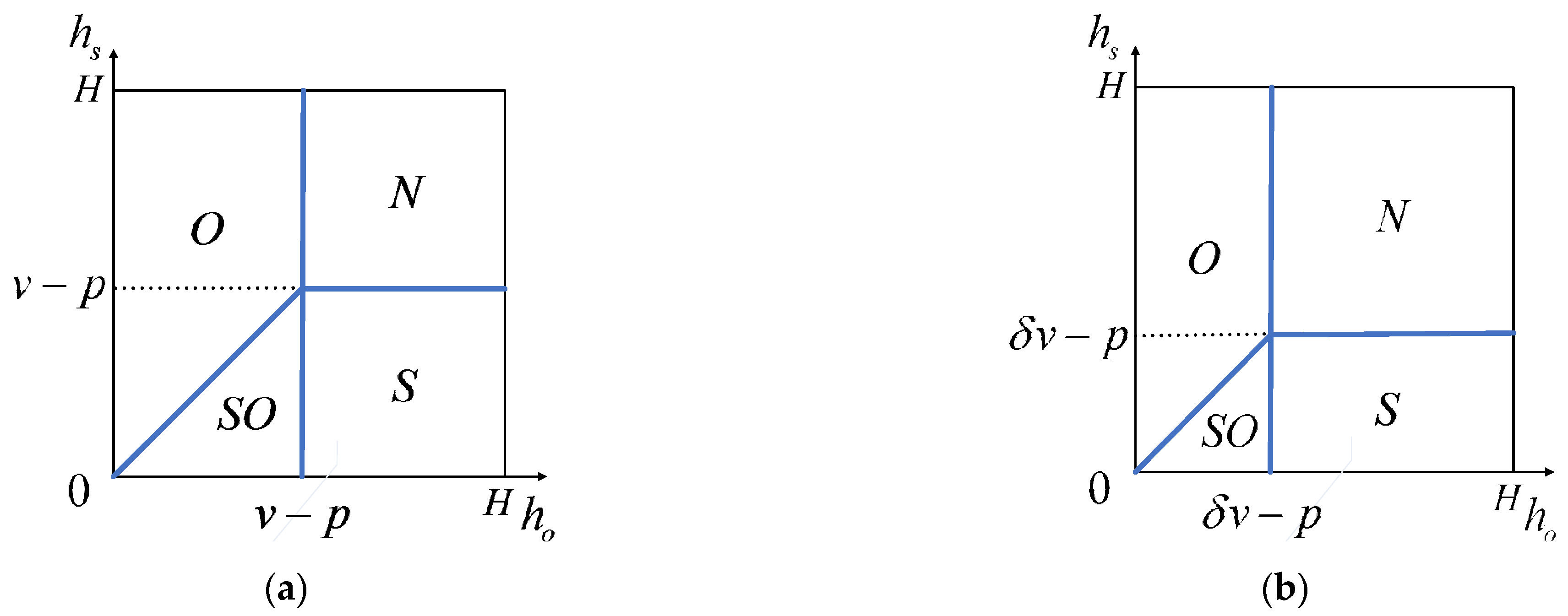
First, we consider the case without a coupon promotion. An H-type customer chooses among four options: purchase online (with utility v p h o ), buy in the BOPS channel (with utility v p h b ), purchase in the store (with utility v p h s ), or no purchase (with utility 0 ). An L-type consumer also chooses from four options: purchase online (with utility δ v p h o ), buy in the BOPS channel (with utility δ v p h b ), purchase in the store (with utility δ v p h s ), or no purchase (with utility 0 ). She makes a choice by maximizing utility. Note that only consumers with a nonnegative online purchase utility will choose to buy online after encountering a stockout in the store, while the rest will leave. Then, there are six market segments for both types of consumers. Specifically, there are “O” customers (who only purchase online), “BO” customers (who choose BOPS if the store has inventory but shift to buying online if they encounter stockouts), “B” customers (who shop in the BOPS channel exclusively), “SO” customers (who buy in the store if the product is available there but buy online otherwise), “S” customers (who buy in the store channel directly), and “N” customers (who do not purchase).
We analyze the H-type consumers first. If consumers’ utilities satisfy v p h o > max ( v p h b , v p h s , 0 ) , they are “O” customers, and their proportion is denoted as α o B H . If consumers’ utilities satisfy v p h b > max ( v p h o , v p h s , 0 ) and v p h o 0 , this segment is “BO” customers, and their proportion is denoted as α b o B H . If consumers’ utilities satisfy v p h b > max ( v p h o , v p h s , 0 ) and v p h o < 0 , these consumers are “B” customers, and their proportion is denoted as α b B H . If consumers’ utilities satisfy v p h s > max ( v p h o , v p h b , 0 ) and v p h o 0 , they are “SO” customers, and their proportion is denoted as α s o B H . If consumers’ utilities satisfy v p h s > max ( v p h o , v p h b , 0 ) and v p h o < 0 , these consumers are “S” customers, and their proportion is denoted as α s B H . For consumers whose utilities satisfy max ( v p h o , v p h b , v p h s ) < 0 , their proportion is denoted as α n B H .
Then, we analyze the six segments in the L-type consumer group. Similarly, for L-type consumers whose utilities satisfy δ v p h o > max ( δ v p h b , δ v p h s , 0 ) , their proportion is denoted as α o B L . If consumers’ utilities satisfy δ v p h b > max ( δ v p h o , δ v p h s , 0 ) and δ v p h o 0 , their proportion is denoted as α b o B L . For L-type consumers whose utilities satisfy δ v p h b > max ( δ v p h o , δ v p h s , 0 ) and δ v p h o < 0 , their proportion is denoted as α b B L . If consumers’ utilities satisfy v p h s > max ( v p h o , v p h b , 0 ) and v p h o 0 , the proportion of this segment is denoted as α s o B L . For L-type consumers whose utilities satisfy v p h s > max ( v p h o , v p h b , 0 ) and v p h o < 0 , α s B L is used to denote their proportion. For L-type consumers whose utilities satisfy max ( δ v p h o , δ v p h b , δ v p h s ) < 0 , their proportion is denoted as α n B L .
There are two situations when calculating the six segments of the H-type and L-type consumers, as shown in Figure 1 and Figure 2.
(1)
When β o + β s 1 , each market segment of the two types of consumers is shown in Figure 1. We denote the proportions of the six segments for the two types of consumers as α o m 1 , α b o m 1 , α b m 1 , α s o m 1 , α s m 1 , and α n m 1 , respectively, where m = B H , B L . From Figure 1, we can calculate α o m 1 , α b o m 1 , α b m 1 , α s o m 1 , α s m 1 , α n m 1 , and show them in Appendix B.
(2)
When β o + β s > 1 , each market segment of the two types of consumers is depicted in Figure 2. In this situation, we denote the proportions of the six segments for the two types of consumers as α o m 2 , α b o m 2 , α b m 2 , α s o m 2 , α s m 2 , and α n m 2 , respectively, where m = B H , B L . From Figure 2, we derive α o m 2 , α b o m 2 , α b m 2 , α s o m 2 , α s m 2 , and α n m 2 and show them in Appendix B.
We use α t B k = λ ( α b o B H k + α b B H k + α s o B H k + α s B H k ) + ( 1 λ ) ( α b o B L k + α b B L k + α s o B L k + α s B L k ) ,   k = 1 , 2 to denote the proportion of consumers who require store inventory to meet their demand in the nonpromotional case. The expected profit function of the brand is given by:
π B k ( q B k ) = p E min ( α t B k D , q B k ) c q B k + r E min ( α t B k D , q B k ) + p E [ λ α o B H k + ( 1 λ ) α o B L k ] D + p E ( λ ( α b o B H k + α s o B H k ) + ( 1 λ ) ( α b o B L k + α s o B L k ) α t B k ) ( α t B k D q B k ) + ,   k = 1 , 2
In Equation (1), the first three terms represent the profits brought to the brand by consumers who visit the store. The fourth item refers to the profit that the brand obtains from consumers who prefer purchasing online, and the fifth term represents the profit that the brand obtains from consumers who tend to visit the store but have to purchase online due to shortages of the product. Then, the brand’s optimal store inventory decision in the nonpromotional case can be derived, i.e., Proposition 3.
Proposition 3. 
When β o + β s 1 , if 0 < c < r + F p , then q B * = A F ¯ 1 ( c r + F p ) ; otherwise, q B * = 0 . When β o + β s > 1 , if 0 < c < r + J p , then q B * = G F ¯ 1 ( c r + J p ) ; otherwise, q B * = 0 . A , F , G and J are constants defined in the Appendix A.
Then, we consider the case with a coupon promotion. Note that H-type consumers never use coupons, and a coupon promotion only changes the utilities of L-type consumers; hence, we next analyze L-type consumers. Recall that the redemption cost of L-type consumers is normalized to zero, and they always use coupons when available. An L-type customer chooses among four options: purchase online (with utility δ v p + f h o ), purchase in the BOPS channel (with utility δ v p + f h b ), purchase in the store channel (with utility δ v p h s ), or no purchase (with utility 0). There are six segments in the L-type consumer market. For L-type consumers whose utilities satisfy δ v p + f h o > max ( δ v p + f h b , δ v p h s , 0 ) , their proportion is denoted as α o L . If consumers’ utilities satisfy δ v p + f h b > max ( δ v p + f h o , δ v p h s , 0 ) and δ v p + f h o 0 , α b o L represents their proportion. For L-type consumers whose utilities satisfy δ v p + f h b > max ( δ v p + f h o , δ v p h s , 0 ) and δ v p + f h o < 0 , their proportion is denoted as α b L . If consumers’ utilities satisfy δ v p h s > max ( δ v p + f h o , δ v p + f h b , 0 ) and δ v p + f h o 0 , we use α s o L to denote their proportion. For L-type consumers whose utilities satisfy δ v p h s > max ( δ v p + f h o , δ v p + f h b , 0 ) and δ v p + f h o < 0 , α s L refers to their proportion. Finally, we use α n L to denote the proportion of consumers whose utilities satisfy max ( δ v p + f h o , δ v p + f h b , δ v p h s ) < 0 .
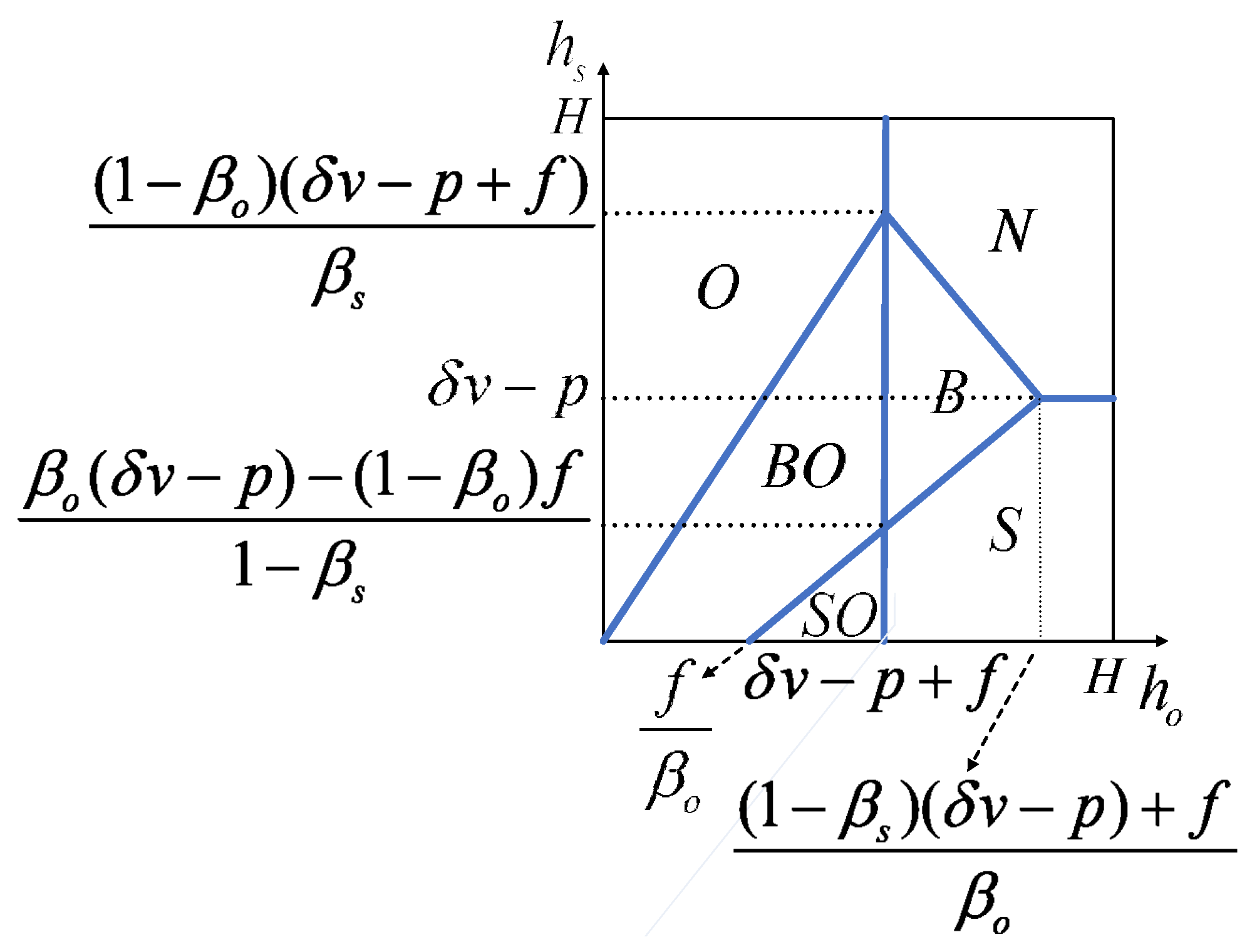
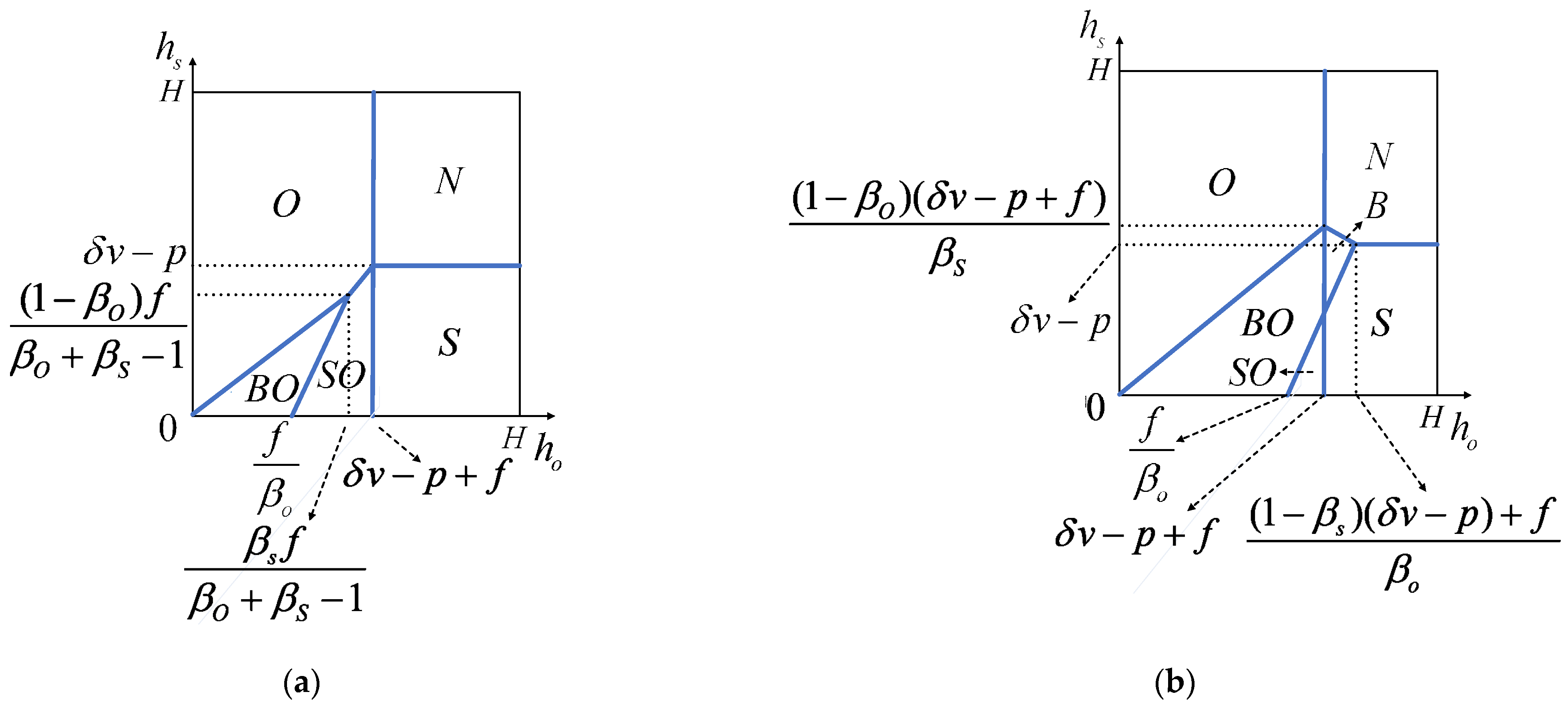
There are two situations when solving for the sizes of six market segments for the two types of consumers, as shown in Figure 3 and Figure 4. The coupon face value in both situations is represented as f j ,   j = 1 , 2 .
(1)
When β o + β s 1 , the market segmentation of L-type consumers is depicted in Figure 3. In this situation, the proportions of these six segments are denoted as α o L 1 , α b o L 1 , α b L 1 , α s o L 1 , α s L 1 , and α n L 1 . From Figure 3, we obtain α o L 1 , α b o L 1 , α b L 1 , α s o L 1 , α s L 1 , and α n L 1 and show them in Appendix B.
(2)
When β o + β s > 1 , Figure 4 demonstrates the market segmentation of L-type consumers. In this situation, the proportions of these six segments are denoted as α o L 2 , α b o L 2 , α b L 2 , α s o L 2 , α s L 2 and α n L 2 . From Figure 4, we observe that if f 2 < ( β o + β s 1 ) ( δ v p ) 1 β o , the market segmentation of L-type consumers can be calculated and shown in Appendix B. Similarly, if f 2 ( β o + β s 1 ) ( δ v p ) 1 β o , the market segmentation of L-type consumers can also be counted and shown in Appendix B.
The corresponding utilities of an H-type consumer’s four choices are the same as those in the nonpromotional case, so the proportions of the six segments for the H-type consumers in the two cases are α i H 1 = α i B H 1 and α i H 2 = α i B H 2 , where i = o , b o , b , s o , s , n . The proportion of consumers requiring store inventory to meet demand in the promotional case is expressed as α t j = λ ( α b o H j + α b H j + α s o H j + α s H j ) + ( 1 λ ) ( α b o L j + α b L j + α s o L j + α s L j ) ,   j = 1 , 2 , and the brand faces the following profit function:
π i ( q j , f j ) = ( p ( 1 λ ) ( α b o L j + α b L j ) f j α t j ) E min ( α t j D , q j ) c q j + r E min ( α t j D , q j ) + p E λ α o H D + ( p f j ) E ( 1 λ ) α o L j D + λ ( α b o H j + α s o H j ) p + ( 1 λ ) ( α b o L j + α s o L j ) ( p f j ) α t i E ( α t j D q j ) + ,   j = 1 , 2
Because the L-type consumers who eventually purchase through the BOPS channel redeem coupons, the first two terms of Equation (2) represent the expected newsvendor profit obtained from selling products. The brand’s cross-selling revenues are shown in the third term. The fourth and fifth terms represent the profits from the H-type and L-type consumers who are inclined to purchase online. The last part captures the profit that is contributed by consumers who eventually purchase online after finding that the store does not have inventory.
Emmons and Gilbert [63] and Jadidi et al. [33] confirmed that π ( q , f ) is a concave function in coupon face value f and inventory level q , but is not jointly concave in f and q . Consistent with many studies, such as Lau et al. [64] and Jadidi et al. [65], we take two steps to find the solutions. First, we calculate the unique optimal solution of q by solving Equation (2), and it is a function of f . Second, we replace q in π ( q , f ) with the optimal solution of q . As a result, π ( q , f ) only contains a decision variable f . Specifically, by taking f as given and solving Equation (2), we derive the optimal value q j * = α t j F ¯ 1 ( α t j c ( λ ( α b H j + α s H j ) + ( 1 λ ) ( α b L j + α s L j ) ) p + ( 1 λ ) ( α s o L j α b L j ) f j + α t j r ) ,   j = 1 , 2 . Then, q j * is substituted into Equation (2). However, it is difficult for us to derive the closed-form optimal solution of f because the expression of q j * contains the inverse cumulative distribution function. Therefore, we obtain the optimal decisions q j * and f j * through numerical experiments in Section 4.

4. Numerical Analysis

In this section, we numerically analyze the coupon promotion and inventory strategies of an omnichannel brand when consumers’ online and store hassle costs are both heterogeneous. We first use examples to demonstrate the existence of the optimal decision when the brand issues coupons and then focus on the conditions for the brand to offer a promotion. Finally, we examine the influence of model parameters on the equilibrium results. We assume that the market demand follows a uniform distribution on [ 0 , 10 ] , which has been widely adopted in the literature. The software MATLAB is used to conduct the following numerical analysis. Consistent with practice, the parameters are set as follows: β o ( 0 , 1 ) , β s ( 0 , 1 ) , c = 0.01 , δ ( 0 , 1 ) , λ = 0.8 , p ( 0.1 , 0.9 ) , v = 1 , r = 0.2 and H = 10 . For example, a product price that is either too high or too low is unrealistic.

4.1. Joint Decision of Coupon Face Value and Store Inventory When the Brand Offers Coupons

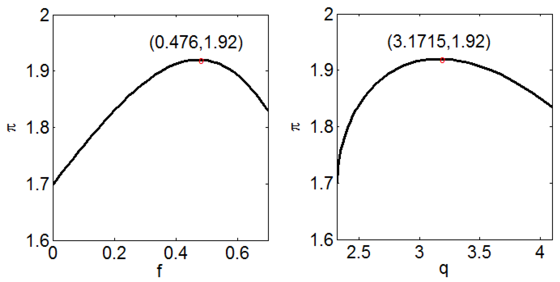
We now explore how to set the coupon face value and store inventory to maximize the brand’s profit when coupons are offered. In this section, we set p = 0.7 and d = 0.72 . Then, we take β o = β s = 0.4 and β o = β s = 0.6 in Figure 5 and Figure 6 as examples to illustrate the optimal coupon face value and inventory decisions when the brand issues coupons.
Figure 5 indicates that when β o = β s = 0.4 , i.e., β o + β s = 0.8 < 1 , the brand’s profit first increases and then decreases with f and q . The optimal coupon face value and store inventory level are f * = 0.476 and q * = 3.1715 , respectively. Here, the brand achieves the maximum profit ( π * = 1.92 ).
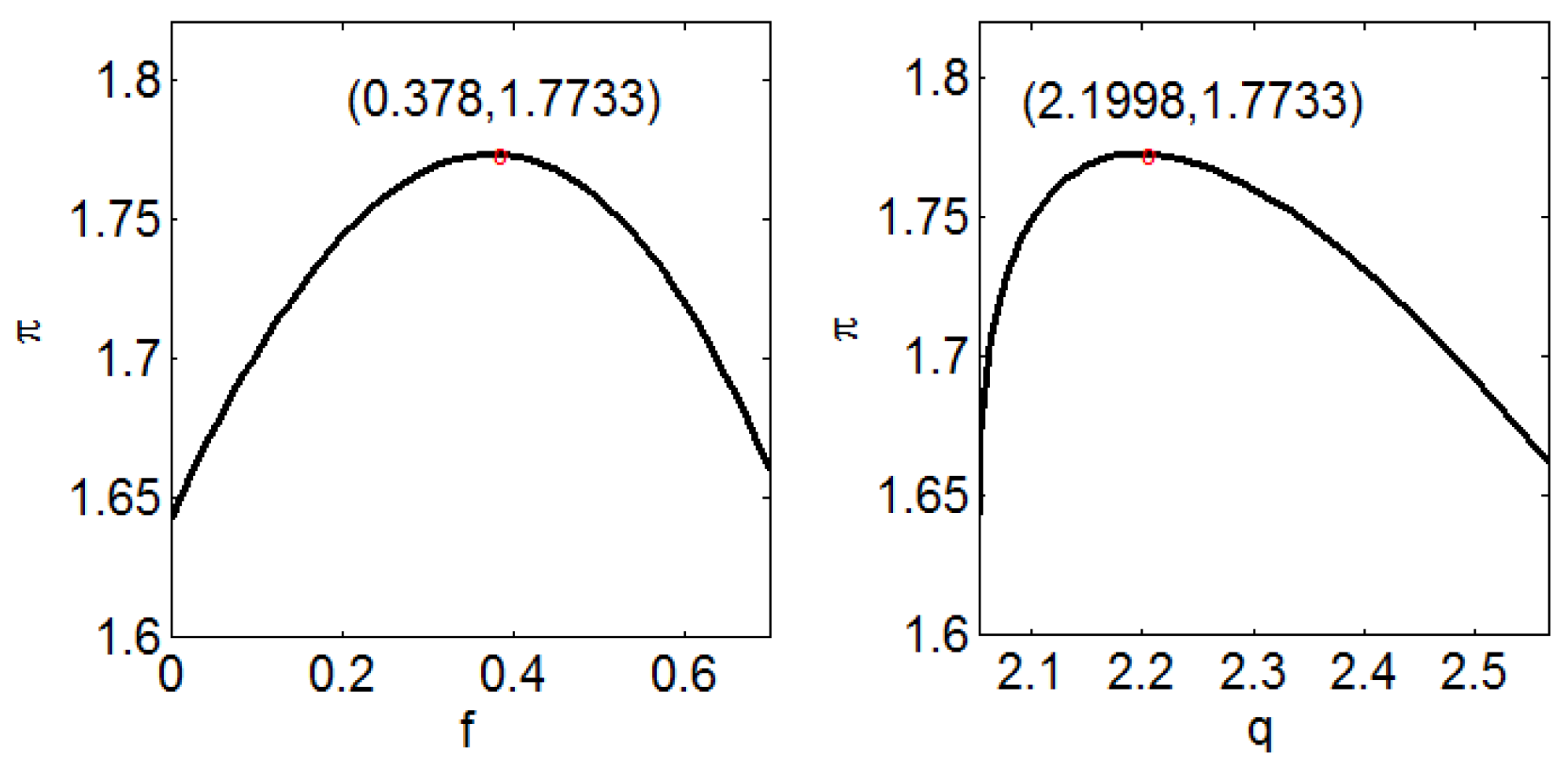
Similarly, Figure 6 shows that when β o = β s = 0.6 , i.e., β o + β s = 1.2 > 1 , there exists an optimal coupon face value f * = 0.378 and an optimal store inventory level q * = 2.1998 with a maximum profit π * = 1.7733 . Comparing Figure 5 and Figure 6 reveals that the optimal coupon face value, inventory level and profit when β o = β s = 0.6 are lower than those when β o = β s = 0.4 . The reason for this finding relates to the fact that the hassle cost in the BOPS channel increases with β o + β s . Then, fewer consumers choose to use coupons in the BOPS channel, resulting in lower store inventory and profit. As a result, the brand reduces the coupon face value to maintain high marginal revenue during the promotion. Furthermore, it can be found that different hassle costs in the BOPS channel lead to differences in the impacts of coupon promotions on offline demand and profits, i.e., the higher the hassle costs, the lower the offline demand and profit increase from digital coupon promotions.

4.2. Digital Coupon Promotion Strategy of the Brand: Promote or Not

In this part, we explore when the brand should release digital coupons in the online and BOPS channels by comparing its profits with and without a coupon promotion. The results are depicted in Figure 7. The z-axis represents the difference in the brand’s profits between when it does and does not conduct the coupon promotion, and Figure 7 shows the influence of the price p and the valuation coefficient of L-type consumers for products relative to H-type consumers δ on the profit difference. The brand offers digital coupons only when the profit in the promotional case is higher than that in the nonpromotional case.
Figure 7 demonstrates that in the scenario with heterogeneous online and store hassle costs, the brand should adopt the coupon promotion when the product price p is high or p is moderate and the coefficient of the difference in valuation between two types of consumers 1 δ is high. This does not contradict the conclusion that the brand benefits from the coupon promotion when both p and δ are high in the homogeneous scenario. When price p is high and there is no coupon promotion, L-type consumers will buy products with coupons only if their valuation δ v is greater than the hassle cost in the online or BOPS channel in the homogeneous scenario. However, in the heterogeneous scenario, there always exists a low online or BOPS hassle cost, which enables coupon promotions to induce new purchases. Therefore, the condition for a coupon promotion in the heterogeneous scenario is looser. In addition, in the homogeneous scenario, when p is moderate and there is no coupon promotion, the brand has no motivation to promote since the market is fully covered. In contrast, in the heterogeneous scenario, the lower δ is, the more significant the increased revenue from the coupon promotion is for the brand due to the enhanced price discrimination effect. Moreover, comparing Figure 7a,b shows that although the profit difference decreases with β o + β s , β o + β s has little influence on the brand’s decision of whether to engage in a coupon promotion.
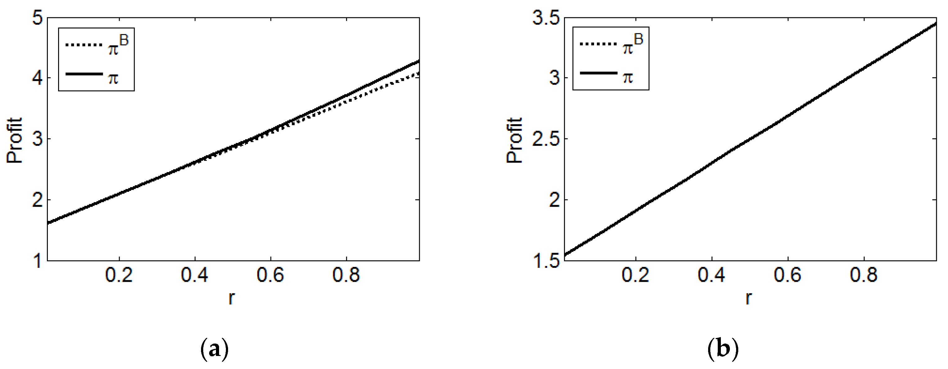
In an omnichannel context, we also investigate the impact of cross-channel revenue r on the brand’s coupon promotion strategy in Figure 8. We set p = 0.4 and r ( 0 , 1 ) .
From Figure 8a, when r surpasses a certain threshold, the brand’s profit with a coupon promotion is higher than that without coupon promotion. The larger r is, the more likely the brand is to issue coupons in the online and BOPS channels. This is because when the cross-channel revenue is high, the brand sees a large profit increase from the L-type consumers who purchase through the BOPS channel with coupons. Additionally, in Figure 8b, the profit curves of the brand in the promotional and nonpromotional cases coincide, indicating that the brand does not conduct a coupon promotion in this setting. Furthermore, the larger β o + β s is, the greater the possibility is that the brand will engage in a coupon promotion. The reason for this finding is that a larger β o + β s means a higher BOPS hassle cost, fewer consumers using coupons to buy in the BOPS channel, and a smaller market share increase from the coupon promotion.

4.3. Sensitivity Analysis

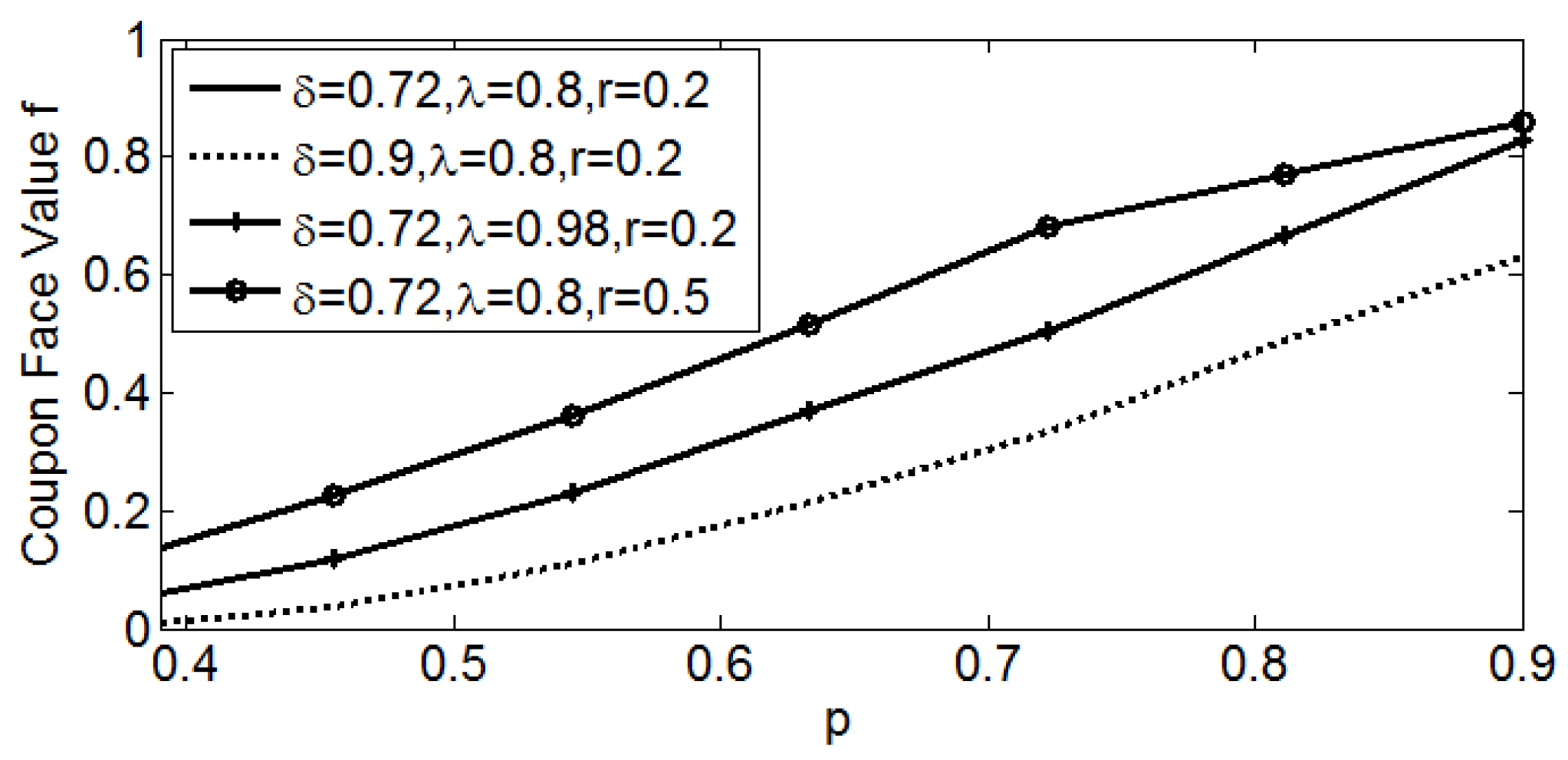
We present numerical studies to assess the impacts of the model parameters on the brand’s optimal decisions (i.e., coupon face value and store inventory level) and profit to derive managerial insights. The results and insights in the case of β o = β s = 0.6 are similar to those in the case of β o = β s = 0.4 ; hence, we only include the case of β o = β s = 0.4 here for brevity. First, we analyze the impacts of p , δ , λ , and r on the coupon face value when coupons are distributed. The results are presented in Figure 9. The value of p ensures that the brand is willing to issue coupons in all scenarios.
In Figure 9, the curve of δ = 0.72 ,   λ = 0.8 ,   r = 0.2 coincides with the curve of δ = 0.72 ,   λ = 0.98 ,   r = 0.2 due to the intuition that the coupon face value is unrelated to the proportion of H-type consumers when the coupon promotion is conducted. We can also observe from Figure 9 that the coupon face value increases with p and r , while it decreases with δ . The rationale is that the brand has to raise its coupon promotion effort to compete for market share. In the same way, a larger δ indicates a higher valuation of the L-type consumers for products. Accordingly, the brand only needs to provide a small coupon face value to ensure that L-type consumers are attracted to increase marginal revenue. Furthermore, due to the cross-channel revenue from the L-type consumers who use BOPS with coupons, a larger r encourages the brand to issue coupons with higher face value to capture more L-type consumers and obtain higher profit.
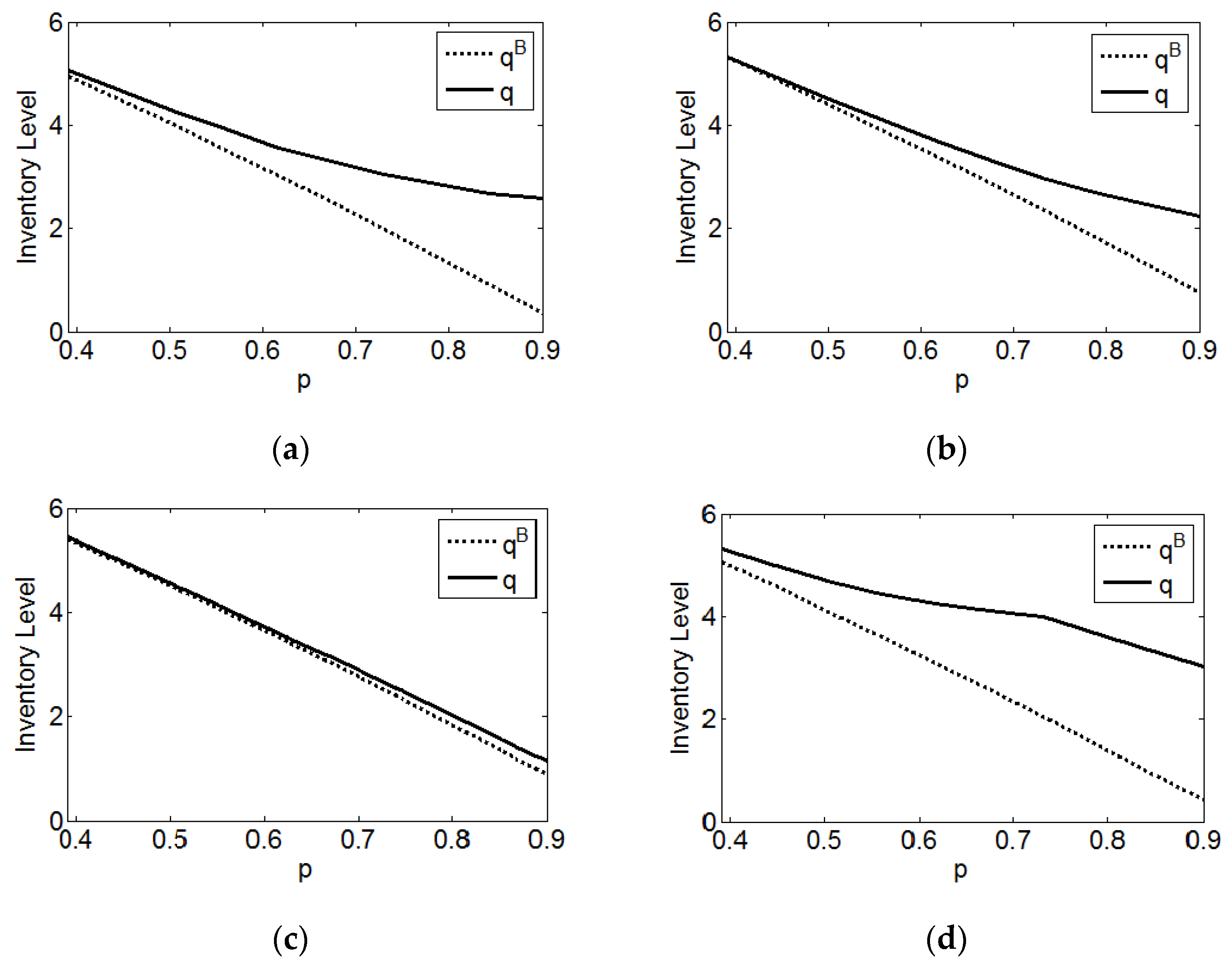
Then, we consider the impacts of p , δ , λ , and r on store inventory. q and q B denote the store inventory level when the brand is promoting and not promoting, respectively. The value of p makes it possible for the brand to offer coupons in all scenarios.
As shown in Figure 10, the store inventory in the promotional case is always higher than that in the nonpromotional case. This does not contradict the previous finding that when the proportion of H-type consumers is high, the unit inventory cost is not too high and the price is high, coupon promotion reduces store inventory in the scenario of homogeneous online and store hassle costs. This is because in the heterogeneous scenario, some L-type consumers still purchase even if there are no coupons in the market. When the brand initiates the coupon promotion, the reduction in profit generated by unit inventory decreases, and the inventory-reducing effect is relatively small compared with the homogeneous scenario, thus increasing store inventory. In addition, when price p is low, store inventory difference q q B is very small, and the difference gradually becomes significant with an increase in p . This is because when p is low, there are few L-type consumers who cannot afford the product in the nonpromotional case, and the coupon promotion has no notable market coverage expansion effect. Hence, the brand slightly increases its store inventory. Furthermore, the brand stocks less with an increase in p due to the shrinking market share.
Interestingly, comparing Figure 10a,b and Figure 10a,c reveals that although q B increases with δ and λ and q q B decreases with δ and λ , the change in q with respect to δ and λ is related to p . Specifically, q increases with δ and λ when p is low, while it decreases with δ and λ when p is high. This is because both δ and λ have two impacts on store inventory. On the one hand, a larger δ or λ means more sales, and the brand needs to arrange more products in its stores regardless of whether digital coupons are issued. On the other hand, a smaller δ or λ means a smaller market share when there is no coupon promotion, more L-type consumers who are attracted to buy products with coupons in the BOPS channel, a larger inventory increase required by consumers caused by the coupon promotion, and higher store inventory. When p is high, the market coverage expansion effect of coupon promotion is sufficiently large that the latter influence dominates the former. Finally, Figure 10 also suggests that q , q B , and q q B increase with r . The basic principle is that the brand tends to place more inventory in the store to attract more consumers to shop in the BOPS and store channels when r becomes larger.
Figure 11 illustrates how the profits of the brand with and without promotion π and π B vary with p , δ , λ , and r .
Obviously, the brand’s profit first increases and then decreases with p regardless of whether coupons are issued, suggesting that a moderate price contributes to a high profit. Regarding the impacts of δ and λ , it is intuitive that π B increases with δ and λ since a large δ or λ can bring high product sales. In particular, Figure 11 shows that π always increases with δ and increases with λ when p is low, while it decreases with λ when p is high. We explain this as follows: on the one hand, previous analysis indicates that the market share and store inventory increase with λ and δ when the price is low because of the weak market coverage expansion effect of coupon promotion, while they decrease with λ and δ when the price is high. On the other hand, because the coupon face value is irrelevant to λ but negatively related to δ , the brand’s marginal profit increases with δ in the promotional case, and this positive impact of δ is greater than the negative impact mentioned previously. Therefore, only when the price is low can the brand obtain more profit from the larger λ , while it can always benefit more from a larger δ . Similar to δ , Figure 11 shows that π π B decreases with λ . This is because the higher p is, the weaker the market coverage expansion effect of coupons, and the lower the increased revenue of the brand. Additionally, the result that the profit difference π π B increases with p and r but decreases with δ is consistent with Figure 7 and Figure 8.

5. Conclusions, Managerial Insights, and Discussions

Omnichannel retailing has become prevalent in recent years. Many brands have introduced BOPS. Therefore, this paper conducts analytical research to explore whether and how a brand should issue digital coupons in the online and BOPS channels and the corresponding decisions of coupon face value and store inventory level. We consider the two scenarios where consumers have homogeneous and heterogeneous hassle costs in the online and store channels and characterize the price discrimination effect of a coupon promotion.
Results show that in the homogeneous scenario, the brand benefits from the promotional campaign when both p and δ are large. Similarly, in the heterogeneous scenario, a coupon promotion is profitable for the brand when p is large or p is moderate but δ is small. A higher cross-selling revenue r enhances the brand’s preference for distributing coupons. In addition, a coupon promotion may decrease inventory in the homogeneous scenario but always motivates the brand to stock more inventory in the heterogeneous scenario. However, when the brand issues digital coupons, hassle cost in the BOPS channel always reduces the increment of offline demand and profit. As for the coupon face value, it increases with p and r , while it decreases with δ . Furthermore, in the nonpromotional case, inventory increases with δ , λ and r while it decreases with p and has nothing to do with λ . In the promotional case, inventory increases with r , decreases with p , and increases with δ and λ only when p is small. Finally, the profit of the brand first increases and then decreases with p and increases with δ and r regardless of whether it offers a promotion. Specifically, if coupons are issued, the profit increases with λ when p is small but decreases with λ when p is large.
Based on these main findings, we obtain the following managerial insights for brands that sell products in countries with the permission of price discrimination or adopt some legitimate forms (limited-time coupons).
First, our findings underscore the importance of the price, the valuation difference between the two types of consumers in the market and the cross-selling revenue to the success of an omnichannel brand’s promotional campaign of offering digital coupons in the online and BOPS channels. The distribution of coupons does not always generate a higher profit in the omnichannel context, in contrast to the previous research by Li et al. [11], which argued that an omnichannel retailer’s profit will be increased by the coupon promotion mentioned in this paper. Hence, the brand must be cautious when implementing the promotion, and accurate estimations of these key factors could help it gain more profit.
Second, in practice, store and online hassle costs usually differ across customers. In this situation, before coupons are issued in the online and BOPS channels, the brand should carry more products in the store in advance. In addition, the store inventory should be dynamically adjusted according to changes in price, cross-selling revenue. and consumer market characteristics regardless of whether the brand offers a promotion. In particular, whether the brand should increase or decrease inventory with a higher proportion of price-insensitive consumers or a higher coefficient of the difference in valuation between two types of consumers depends on the price. Moreover, the brand should simplify the purchase and pickup process to reduce the hassle cost of the BOPS channel, thus enhancing the effectiveness of digital coupon promotions and earning more profits.
Third, when conducting a coupon promotion, the brand can reduce its coupon promotion efforts if the price or the coefficient of the difference in valuation between two types of consumers or the cross-selling revenue is lower. The brand does not need to change its promotional efforts when the proportion of price-insensitive consumers varies.
Finally, in both the promotional and nonpromotional cases, the brand gains high profit when the price is moderate. Furthermore, an increased proportion of price-insensitive consumers is not always beneficial when coupons are offered. We also suggest that the brand should make efforts to increase the cross-selling revenue and the coefficient of the difference in valuation between two types of consumers to enhance its profitability. Specifically, the brand can initiate more free experience activities for goods in stores and pay for advertising to improve price-sensitive consumers’ assessment of the product.
Our findings are in accord with previous studies indicating that price promotions benefit firms when the price is high or moderate, and price elasticity is high. However, we contribute to the literature on coupon promotion by verifying the effect of hassle costs on brands’ strategies and profits and identifying the interaction between digital coupon policy and inventory management in omnichannel retailing. Although we believe this to be the first research to explore the joint decision of digital coupon promotion and store inventory in an omnichannel environment, the present paper has limitations and several potential directions that merit future research. First, we assume that the price is exogenously given due to market equilibrium conditions or the determination of price at the moment when the product is finished. Generalizing the results to the case where the price is a decision variable would be an interesting topic. Second, we assume that the brand offers coupons with a common face value in the online and BOPS channels when it conducts a promotion. However, Li et al. [11] reported that offering coupons with a different face value is optimal. Therefore, research considering the case where coupons are provided with a different face value could be conducted in the future to generalize the current study and generate more insights for brands. Furthermore, we do not consider the influence of coupon distribution and redemption costs on the brand’s joint decision. Incorporating these costs into the model may present different results since these costs can significantly influence the brand’s coupon promotion strategy [6].

Author Contributions

Conceptualization, Y.Z. and X.H.; methodology, Y.Z.; software, Y.Z.; validation, Y.Z. and X.H.; formal analysis, Y.Z.; investigation, Y.Z. and X.H.; writing—original draft preparation, Y.Z.; writing—review and editing, Y.Z. and X.H.; supervision, X.H.; funding acquisition, X.H. All authors have read and agreed to the published version of the manuscript reported.

Funding

This research was funded by the National Natural Science Foundation of China for grant number 72171067.

Data Availability Statement

Not applicable.

Acknowledgments

The author would like to thank the authors for the reference materials.

Conflicts of Interest

The authors declare no conflict of interest.

Appendix A

Proof of Proposition 1. 
We first analyze the condition for the case where the brand does not offer digital coupons and the corresponding optimal inventory decision. From the previous analysis, we know that when the brand adopts a low-price strategy that induces all consumers to purchase even if no coupon is issued, the brand is not willing to promote. There are three specific situations to discuss.
(1)
When h o < min ( h b , h s ) , because the product sales volume should not be zero in the nonpromotional case, the brand sets price p = δ v h o . Then, all consumers shop online; hence, q B * = 0 .
(2)
When h b < min ( h o , h s ) , if the brand does not conduct a coupon promotion, there are two pricing strategies: p = δ v h b and p = δ v h o . When p = δ v h b and v > h o h b 1 δ , all consumers prefer using BOPS, while H-type consumers switch to online after finding that the store is out of stock, but L-type consumers directly leave. Then, the brand’s expected profit function is π = ( p + r ) E min ( D , q ) c q + p E λ ( D q ) + . The first term represents the profit from consumers who have obtained products by using BOPS. The second item is the inventory cost, and the last item is the profit from the H-type consumers who switch to purchasing online after encountering a stockout in the store. We maximize the profit function and derive that if c < ( 1 λ ) ( δ v h b ) + r , then q B * = F ¯ 1 ( c ( 1 λ ) ( δ v h b ) + r ) ; otherwise, q B * = 0 since H-type consumers shop online and L-type consumers leave. When p = δ v h b and v h o h b 1 δ , all consumers prefer using BOPS and leaving after encountering a stockout in the store. Then, the brand’s expected profit function is π = ( p + r ) E min ( D , q ) c q . We can derive that if c < δ v h b + r , then q B * = F ¯ 1 ( c δ v h b + r ) ; otherwise, q B * = 0 . When p = δ v h o , all consumers prefer using BOPS and switching to purchasing online after encountering a stockout in the store, and the brand’s expected profit function is π = ( p + r ) E min ( D , q ) c q + p E ( D q ) + . We can calculate that if c < r , then q B * = F ¯ 1 ( c r ) ; otherwise, q B * = 0 .
(3)
When h s < min ( h o , h b ) , if the brand does not conduct a coupon promotion, there are two pricing strategies: p = δ v h s and p = δ v h o . Similar to (2), we can obtain that when h s < min ( h o , h b ) , p = δ v h s and v > h o h s 1 δ , if c < ( 1 λ ) ( δ v h s ) + r , then q B * = F ¯ 1 ( c ( 1 λ ) ( δ v h s ) + r ) ; otherwise, q B * = 0 . When h s < min ( h o , h b ) , p = δ v h s and v h o h s 1 δ , if c < δ v h s + r , then q B * = F ¯ 1 ( c δ v h s + r ) ; otherwise, q B * = 0 . When h s < min ( h o , h b ) and p = δ v h o , if c < r , then q B * = F ¯ 1 ( c r ) ; otherwise, q B * = 0 .
Then, we explore the condition for the brand to offer a coupon promotion. From the previous analysis, we know that the brand offers such a promotion only when its price is so high that only H-type consumers purchase without coupons. The following three specific cases are discussed.
(1)
When h o < min ( h b , h s ) , all consumers prefer the online channel. Then, if p = v h o , only H-type consumers shop online. In this instance, coupons can encourage L-type consumers to buy and thus increase the brand’s profit. Therefore, the brand issues coupons.
(2)
When h b < min ( h o , h s ) , all consumers prefer using BOPS. If p = v h b , only H-type consumers choose to buy in the BOPS channel and leave if they encounter a stockout in the store. Then, the brand offers coupons to encourage L-type consumers to shop in the BOPS or online channel. If p = v h o and v > h o h b 1 δ , only H-type consumers tend to use BOPS and switch to online if the store is out of stock. In this situation, the brand’s profit increases if it distributes coupons in the online and BOPS channels to entice new purchases from L-type consumers. In summary, when h b < min ( h o , h s ) , if p = v h b , or p = v h o and v > h o h b 1 δ , the brand issues coupons.
(3)
When h s < min ( h o , h b ) , all consumers prefer the BOPS channel. Similar to (2), if p = v h s , or p = v h o and v > h o h s 1 δ , only H-type consumers shop in the store channel, and the brand issues coupons.
Finally, we study the optimal coupon face value f * and store inventory level q * when the brand distributes coupons. Five specific situations are discussed here.
(1)
When h o < min ( h b , h s ) and p = v h o , since δ v p + f h o > max ( δ v p + f h b , δ v p h s ) , an L-type consumer obtains the maximum utility from buying online with a coupon, and the utility should be nonnegative, that is, δ v p + f h o = f ( 1 δ ) v 0 , f ( 1 δ ) v . All consumers shop online. Hence, the brand’s expected profit function is π = ( p ( 1 λ ) f ) E D and decreases with f . Then, we can derive that if h o < δ v ( p > f ), f * = ( 1 δ ) v and q * = 0 by maximizing the function.
(2)
When h b < min ( h o , h s ) and p = v h b , since δ v p + f h b > max ( δ v p + f h o , δ v p h s ) , an L-type consumer obtains the maximum utility from buying in the BOPS channel with a coupon, and the utility should be nonnegative, that is, δ v p + f h b 0 , f p + h b δ v . When an L-type consumer obtains nonnegative utility from purchasing online, i.e., δ v p + f h o 0 , then f p + h o δ v . Therefore, there are two coupon strategies for the brand. One is to issue coupons with a small face value so that L-type consumers leave after encountering a stockout in the BOPS channel. Here, the brand’s expected profit function is π = λ ( p + r ) E min ( D , q ) + ( 1 λ ) ( p + r f ) E min ( D , q ) c q . The first and second terms are the profits from the H-high and L-type consumers who have obtained products by using BOPS, respectively. In line with Su [61] and He et al. [62], coupon face value and inventory decisions can be derived by maximizing the profit function. Given that the profit function decreases with f , we can derive that if h b < δ v ( p f > 0 ) and c < λ v + ( 1 λ ) δ v + r h b , then f * = p + h b δ v = ( 1 δ ) v and q * = F ¯ 1 ( c λ v + ( 1 λ ) δ v + r h b ) , and both types of consumers buy through the BOPS channel. If h b < δ v and λ v + ( 1 λ ) δ v + r h b c < v h b + r , or h b δ v and c < v h b + r , based on the assumption that r > ( 1 λ ) ( δ v h o ) E D + c λ F ¯ 1 ( c v h b + r ) ( v h b ) E min ( λ D , λ F ¯ 1 ( c v h b + r ) ) E min ( λ D , λ F ¯ 1 ( c v h b + r ) ) , the brand does not offer coupons, and only H-type consumers purchase in the BOPS channel, then q B * = λ F ¯ 1 ( c v + r h b ) . If c v h b + r and h o < δ v ( p f > 0 ) , then f * = ( 1 δ ) v + h o h b and q * = 0 , and only L-type consumers purchase online. If c v h b + r and h o δ v , no consumer will buy the product. This situation is not practical and will not be considered. The other strategy is to issue coupons with a large face value to enable L-type consumers to purchase online after encountering stockouts in the BOPS channel. The brand’s expected profit function is π = λ ( p + r ) E min ( D , q ) + ( 1 λ ) ( p + r f ) E min ( D , q ) c q + ( p f ) E ( 1 λ ) ( D q ) + and decreases with f . Therefore, we can calculate that if h o < δ v and c < λ ( v h b ) + r , then f * = p + h o δ v = ( 1 δ ) v + h o h b and q * = F ¯ 1 ( c λ ( v h b ) + r ) . If h o < δ v and λ ( v h b ) + r c < v + r h b , or h o δ v and c < v + r h b , the brand does not offer coupons because r > ( 1 λ ) ( δ v h o ) E D + c λ F ¯ 1 ( c v h b + r ) ( v h b ) E min ( λ D , λ F ¯ 1 ( c v h b + r ) ) E min ( λ D , λ F ¯ 1 ( c v h b + r ) ) , and only H-type consumers purchase in the BOPS channel, then q B * = λ F ¯ 1 ( c v + r h b ) . If c v h b + r and h o < δ v ( p f > 0 ) , then f * = ( 1 δ ) v + h o h b , q * = 0 , and only L-type consumers purchase online. By comparing the profits under the two coupon strategies, we can summarize the results as follows: when h b < min ( h o , h s ) and p = v h b , if h o < δ v , c < λ ( v h b ) + r and λ > λ 1 , where λ 1 = r E min ( D , F ¯ 1 ( c λ ( v h b ) + r ) ) ( δ v + r h b ) E min ( D , F ¯ 1 ( c λ v + ( 1 λ ) δ v + r h b ) ) + ( δ v h o ) E D + c ( F ¯ 1 ( c λ v + ( 1 λ ) δ v + r h b ) F ¯ 1 ( c λ ( v h b ) + r ) ) v ( 1 δ ) E min ( D , F ¯ 1 ( c λ v + ( 1 λ ) δ v + r h b ) ) ( v h b ) E min ( D , F ¯ 1 ( c λ ( v h b ) + r ) ) + ( δ v h o ) E D , or h o < δ v and λ ( v h b ) + r c < λ v + ( 1 λ ) δ v + r h b , or h b < δ v < h o and c < λ v + ( 1 λ ) δ v + r h b , then f * = ( 1 δ ) v and q * = F ¯ 1 ( c λ v + ( 1 λ ) δ v + r h b ) . If h o < δ v , c < λ ( v h b ) + r and λ λ 1 , then f * = ( 1 δ ) v + h o h b and q * = F ¯ 1 ( c λ ( v h b ) + r ) . If h b < δ v and λ v + ( 1 λ ) δ v + r h b c < v h b + r , or h b δ v and c < v h b + r , the brand does not offer coupons, then q B * = λ F ¯ 1 ( c v + r h b ) . If c v h b + r and h o < δ v , then f * = ( 1 δ ) v + h o h b and q * = 0 .
(3)
When h b < min ( h o , h s ) , p = v h o and v > h o h b 1 δ , an H-type consumer prefers using BOPS and shops online if the store is out of stock, and an L-type consumer obtains the maximum utility δ v p + f h b from buying in the BOPS channel with a coupon. Similar to (2), there are two coupon strategies for the brand. One is to offer coupons with a small face value so that L-type consumers leave after encountering a stockout in the BOPS channel. Here, the brand’s expected profit function is π = λ ( p + r ) E min ( D , q ) + ( 1 λ ) ( p + r f ) E min ( D , q ) c q + p E λ ( D q ) + and decreases with f . We assume that r > c F ¯ 1 ( c ( 1 λ ) ( δ v h b ) + r ) + ( 1 λ ) ( δ v h b ) E ( D F ¯ 1 ( c ( 1 λ ) ( δ v h b ) + r ) ) + E min ( D , F ¯ 1 ( c ( 1 λ ) ( δ v h b ) + r ) ) . Next, we can derive that if h b < δ v and c < ( 1 λ ) ( δ v h b ) + r , then f * = ( 1 δ ) v + h b h o and q * = F ¯ 1 ( c ( 1 λ ) ( δ v h b ) + r ) . If h o < δ v and c ( 1 λ ) ( δ v h b ) + r , then f * = ( 1 δ ) v and q * = 0 , and all consumers purchase online. If h b < δ v < h o and c ( 1 λ ) ( δ v h b ) + r , the brand does not offer coupons, and only H-type consumers shop online, then q B * = 0 . If h b δ v and c < r , the brand does not offer coupons, and only H-type consumers purchase in the BOPS channel based on the assumption that r > c F ¯ 1 ( c r ) E min ( D , F ¯ 1 ( c r ) ) , then q B * = λ F ¯ 1 ( c r ) . If h b δ v and c r , the brand does not offer coupons, and only H-type consumers purchase online, then q B * = 0 . The other strategy is to issue coupons with a large face value to enable L-type consumers to shop online after facing a stockout in the BOPS channel. The brand’s expected profit function is π = λ ( p + r ) E min ( D , q ) + ( 1 λ ) ( p + r f ) E min ( D , q ) c q + p E λ ( D q ) + + ( p f ) E ( 1 λ ) ( D q ) + and decreases with f . Therefore, we can derive that if h o < δ v and c < r , then f * = ( 1 δ ) v and q * = F ¯ 1 ( c r ) , and the two types of consumers buy in the BOPS channel. If h o < δ v and c r , then f * = ( 1 δ ) v and q * = 0 , and the two types of consumers buy online. If h o δ v and c < r , the brand does not offer coupons because r > c F ¯ 1 ( c r ) E min ( D , F ¯ 1 ( c r ) ) , and only H-type consumers purchase in the BOPS channel, then q B * = λ F ¯ 1 ( c r ) . If h o δ v and c r , the brand does not offer coupons, and only H-type consumers shop online, then q B * = 0 . By comparing the profits under the two coupon strategies, we can summarize the results as follows: when h b < min ( h o , h s ) , p = v h o and v > h o h b 1 δ , if h o < δ v , c < r and λ > λ 2 , where λ 2 = r E min ( D , F ¯ 1 ( c r ) ) ( δ v + r h b ) E min ( D , F ¯ 1 ( c ( 1 λ ) ( δ v h b ) + r ) ) + ( δ v h o ) E D + c ( F ¯ 1 ( c ( 1 λ ) ( δ v h b ) + r ) F ¯ 1 ( c r ) ) ( δ v h o ) E D ( δ v h b ) E min ( D , F ¯ 1 ( c ( 1 λ ) ( δ v h b ) + r ) ) , or h o < δ v and r c < ( 1 λ ) ( δ v h b ) + r , or h b < δ v < h o and c < ( 1 λ ) ( δ v h b ) + r , then f * = ( 1 δ ) v + h b h o and q * = F ¯ 1 ( c ( 1 λ ) ( δ v h b ) + r ) . If h o < δ v , c < r and λ λ 2 , then f * = ( 1 δ ) v and q * = F ¯ 1 ( c r ) . If h b δ v and c < r , the brand does not offer coupons, then q B * = λ F ¯ 1 ( c r ) . If h o < δ v and c ( 1 λ ) ( δ v h b ) + r , then f * = ( 1 δ ) v and q * = 0 . If h b < δ v < h o and c ( 1 λ ) ( δ v h b ) + r , or h b δ v and c r , the brand does not offer coupons, then q B * = 0 .
(4)
When h s < min ( h o , h b ) and p = v h s , an H-type consumer prefers to buy in the store channel and leave after encountering a stockout in the store. When h s < h o < h b , an L-type consumer should obtain the maximum and nonnegative utility from purchasing online with a coupon, i.e., δ v p + f h o 0 ; then, f ( 1 δ ) v + h o h s . The brand’s expected profit function is π = ( p + r ) E min ( λ D , q ) + ( p f ) E ( 1 λ ) D c q and decreases with f . We can calculate that if h o < δ v and c < v h s + r , then f * = ( 1 δ ) v + h o h s and q * = λ F ¯ 1 ( c v h s + r ) . H-type consumers buy offline, while L-type consumers purchase online. If h o δ v and c < v h s + r , based on the assumption that r > ( 1 λ ) ( δ v h o ) E D + c λ F ¯ 1 ( c v h s + r ) ( v h s ) E min ( λ D , λ F ¯ 1 ( c v h s + r ) ) E min ( λ D , λ F ¯ 1 ( c v h s + r ) ) , the brand does not offer coupons and only H-type consumers purchase in the store channel, then q B * = λ F ¯ 1 ( c v h s + r ) . If h o < δ v and c v h s + r , then f * = ( 1 δ ) v + h o h s and q * = 0 , and only L-type consumers shop online. If h o δ v and c v h s + r , no product is sold, and this situation is not included here. When h s < h b < h o , the brand issues coupons with either a small face value f * = ( 1 δ ) v + h b h s or a large face value f * = ( 1 δ ) v + h o h s . By comparing the profits of the brand under the two coupon strategies and following the previous analysis, we can obtain that when h s < h o < h b and p = v h s , if h o < δ v and c < v h s + r , then f * = ( 1 δ ) v + h o h s and q * = λ F ¯ 1 ( c v h s + r ) . If h o < δ v and c v h s + r , then f * = ( 1 δ ) v + h o h s and q * = 0 . If h o δ v and c < v h s + r , the brand does not offer coupons, then q B * = λ F ¯ 1 ( c v h s + r ) . When h s < h b < h o and p = v h s , if h o < δ v , c < λ ( v h s ) + r and λ > λ 3 , where λ 3 = r E min ( D , F ¯ 1 ( c λ ( v h s ) + r ) ) ( δ v + r ( 1 λ ) h b λ h s ) E min ( D , F ¯ 1 ( c λ v + ( 1 λ ) δ v + r λ h s ( 1 λ ) h b ) ) + ( δ v h o ) E D + c ( F ¯ 1 ( c λ v + ( 1 λ ) δ v + r λ h s ( 1 λ ) h b ) F ¯ 1 ( c λ ( v h s ) + r ) ) v ( 1 δ ) E min ( D , F ¯ 1 ( c λ v + ( 1 λ ) δ v + r λ h s ( 1 λ ) h b ) ) ( v h s ) E min ( D , F ¯ 1 ( c λ ( v h s ) + r ) ) + ( δ v h o ) E D , or h o < δ v and λ ( v h s ) + r c < λ v + ( 1 λ ) δ v + r λ h s ( 1 λ ) h b , or h b < δ v < h o and c < λ v + ( 1 λ ) δ v + r λ h s ( 1 λ ) h b , then f * = ( 1 δ ) v + h b h s and q * = F ¯ 1 ( c λ v + ( 1 λ ) δ v + r λ h s ( 1 λ ) h b ) . If h o < δ v , c < λ ( v h s ) + r and λ λ 3 , then f * = ( 1 δ ) v + h o h s and q * = F ¯ 1 ( c λ ( v h s ) + r ) . If h b < δ v and λ v + ( 1 λ ) δ v + r λ h s ( 1 λ ) h b c < v h s + r , or h b δ v and c < v h s + r , the brand does not offer coupons, then q B * = λ F ¯ 1 ( c v + r h s ) . If c v h s + r and h o < δ v , then f * = ( 1 δ ) v + h o h s and q * = 0 .
(5)
When h s < min ( h o , h b ) , p = v h o and v > h o h s 1 δ , an H-type consumer prefers to buy in the store channel and switches to purchasing online after encountering a stockout in the store. When h s < h o < h b , because v > h o h s 1 δ , an L-type consumer should obtain the maximum and nonnegative utility from purchasing online with a coupon, i.e., δ v p + f h o 0 ; then, f ( 1 δ ) v . The brand’s expected profit function is π = ( p + r ) E min ( λ D , q ) + ( p f ) E ( 1 λ ) D c q + p E ( λ D q ) + and decreases with f . We assume that r > c F ¯ 1 ( c r ) E min ( D , F ¯ 1 ( c r ) ) . We can derive that if h o < δ v and c < r , then f * = ( 1 δ ) v and q * = λ F ¯ 1 ( c r ) . H-type consumers buy offline, while L-type consumers purchase online. If h o < δ v and c r , then f * = ( 1 δ ) v and q * = 0 , and all consumers buy products online. If h o δ v and c < r , the brand does not offer coupons, and only H-type consumers purchase in the store channel because r > c F ¯ 1 ( c r ) E min ( D , F ¯ 1 ( c r ) ) , then q B * = λ F ¯ 1 ( c r ) . If h o δ v and c r , the brand does not offer coupons, and only H-type consumers shop online, then q B * = 0 . When h s < h b < h o , the brand either issues coupons with a small face value f * = ( 1 δ ) v + h b h o or a large face value f * = ( 1 δ ) v . Comparing the brand’s profits under the two coupon strategies reveals that the results when h s < h b < h o , p = v h o , and v > h o h s 1 δ are the same as those when h b < min ( h o , h s ) , p = v h o , and v > h o h b 1 δ , so they are merged.
Proposition 1 is proven. □
Proof of Proposition 2. 
From Proposition 1, there are five situations where the brand provides coupons. Hence, the optimal store inventory levels before and after the coupon promotion in these five situations are compared.
(1)
When h o < min ( h b , h s ) and p = v h o , then f * = ( 1 δ ) v and q * = 0 . If the brand does not offer coupons, then only H-type consumers shop online and q B * = 0 . The coupon promotion has no effect on store inventory.
(2)
When h b < min ( h o , h s ) and p = v h b , if h o < δ v , c < λ ( v h b ) + r and λ > λ 1 , or h o < δ v and λ ( v h b ) + r c < λ v + ( 1 λ ) δ v + r h b , or h b < δ v < h o and c < λ v + ( 1 λ ) δ v + r h b , then f * = ( 1 δ ) v and q * = F ¯ 1 ( c λ v + ( 1 λ ) δ v + r h b ) . If h o < δ v , c < λ ( v h b ) + r and λ λ 1 , then f * = ( 1 δ ) v + h o h b and q * = F ¯ 1 ( c λ ( v h b ) + r ) . If c v h b + r and h o < δ v , then f * = ( 1 δ ) v + h o h b and q * = 0 . When h b < min ( h o , h s ) and p = v h b , if the brand does not offer coupons and c < v h b + r , then q B * = λ F ¯ 1 ( c v h b + r ) . Only H-type consumers use BOPS and leave if the store is out of stock. If c v h b + r , no consumer buys the product in the nonpromotional case, which is not included here. By comparing q * = F ¯ 1 ( c λ v + ( 1 λ ) δ v + r h b ) and q * = F ¯ 1 ( c λ ( v h b ) + r ) with q B * = λ F ¯ 1 ( c v h b + r ) , we can obtain that when h b < min ( h o , h s ) and p = v h b , if h o < δ v , c < λ ( v h b ) + r and λ > max ( λ 1 , λ 4 ) , where λ 4 = F ¯ 1 ( c λ v + ( 1 λ ) δ v + r h b ) F ¯ 1 ( c v h b + r ) ) , or h o < δ v , λ > λ 4 and λ ( v h b ) + r c < λ v + ( 1 λ ) δ v + r h b , or h b < δ v < h o , c < λ v + ( 1 λ ) δ v + r h b and λ > λ 4 , or h o < δ v , c < λ ( v h b ) + r and λ 5 < λ λ 1 , where λ 5 = F ¯ 1 ( c λ ( v h b ) + r ) F ¯ 1 ( c v h b + r ) , then q * < q B * , and the coupon promotion reduces store inventory. Otherwise, it increases or has no effect on store inventory.
(3)
When h b < min ( h o , h s ) , p = v h o and v > h o h b 1 δ , or h s < h b < h o , p = v h o and v > h o h s 1 δ , if h o < δ v , c < r and λ > λ 2 , or h o < δ v and r c < ( 1 λ ) ( δ v h b ) + r , or h b < δ v < h o and c < ( 1 λ ) ( δ v h b ) + r , then f * = ( 1 δ ) v + h b h o and q * = F ¯ 1 ( c ( 1 λ ) ( δ v h b ) + r ) . If h o < δ v , c < r and λ λ 2 , then f * = ( 1 δ ) v and q * = F ¯ 1 ( c r ) . If h o < δ v and c ( 1 λ ) ( δ v h b ) + r , then f * = ( 1 δ ) v and q * = 0 . When h b < min ( h o , h s ) , p = v h o and v > h o h b 1 δ , or h s < h b < h o , p = v h o and v > h o h s 1 δ , if the brand does not offer coupons and c < r , then q B * = λ F ¯ 1 ( c r ) . Only H-type consumers tend to go to the store and switch to online if the store is out of stock. If the brand does not offer coupons and c r , then q B * = 0 . Only H-type consumers shop online. By comparing q * with q B * , we can obtain that when h b < min ( h o , h s ) , p = v h o and v > h o h b 1 δ , or h s < h b < h o , p = v h o and v > h o h s 1 δ , if h o < δ v , c < r and λ > λ 2 , or h o < δ v and r c < ( 1 λ ) ( δ v h b ) + r , or h b < δ v < h o and c < ( 1 λ ) ( δ v h b ) + r , then q * = F ¯ 1 ( c ( 1 λ ) ( δ v h b ) + r ) > q B * since h b < δ v and c < ( 1 λ ) ( δ v h b ) + r . If h o < δ v , c < r and λ λ 2 , then q * = F ¯ 1 ( c r ) > q B * = λ F ¯ 1 ( c r ) . If h o < δ v and c ( 1 λ ) ( δ v h b ) + r , then q * = q B * = 0 . In summary, when h b < min ( h o , h s ) , p = v h o and v > h o h b 1 δ , or h s < h b < h o , p = v h o and v > h o h s 1 δ , the coupon promotion increases or has no effect on store inventory.
(4)
When h s < h o < h b and p = v h s , if h o < δ v and c < v h s + r , then f * = ( 1 δ ) v + h o h s and q * = λ F ¯ 1 ( c v h s + r ) . If h o < δ v and c v h s + r , then f * = ( 1 δ ) v + h o h s and q * = 0 . If the brand does not offer coupons and c < v h s + r , then q B * = λ F ¯ 1 ( c v h s + r ) . Only H-type consumers purchase in the store channel and leave after encountering a stockout in the store. If c v h s + r , then no consumer buys the product in the nonpromotional case, which is not included here. Therefore, when h s < h o < h b and p = v h s , the coupon promotion has no effect on the store inventory. When h s < h b < h o and p = v h s , if h o < δ v , c < λ ( v h s ) + r and λ > λ 3 , or h o < δ v and λ ( v h s ) + r c < λ v + ( 1 λ ) δ v + r λ h s ( 1 λ ) h b , or h b < δ v < h o and c < λ v + ( 1 λ ) δ v + r λ h s ( 1 λ ) h b , then q * = F ¯ 1 ( c λ v + ( 1 λ ) δ v + r λ h s ( 1 λ ) h b ) and f * = ( 1 δ ) v + h b h s . If h o < δ v , c < λ ( v h s ) + r and λ λ 3 , then f * = ( 1 δ ) v + h o h s and q * = F ¯ 1 ( c λ ( v h s ) + r ) . If c v h s + r and h o < δ v , then f * = ( 1 δ ) v + h o h s and q * = 0 . If the brand does not offer coupons and c < v h s + r , then q B * = λ F ¯ 1 ( c v h s + r ) . Only H-type consumers purchase in the store channel and leave after encountering a stockout in the store. The case of c v h s + r is not considered here since it is not practical. By comparing q * with q B * , we can obtain that when h s < h b < h o and p = v h s , if h o < δ v , c < λ ( v h s ) + r and λ > max ( λ 3 , λ 6 ) , where λ 6 = F ¯ 1 ( c λ v + ( 1 λ ) δ v + r λ h s ( 1 λ ) h b ) F ¯ 1 ( c v h s + r ) , or h o < δ v , λ > λ 6 and λ ( v h s ) + r c < λ v + ( 1 λ ) δ v + r λ h s ( 1 λ ) h b , or h b < δ v < h o , λ > λ 6 and c < λ v + ( 1 λ ) δ v + r λ h s ( 1 λ ) h b , or h o < δ v , c < λ ( v h s ) + r and λ 7 < λ λ 3 , where λ 7 = F ¯ 1 ( c λ ( v h s ) + r ) F ¯ 1 ( c v h s + r ) , then q * < q B * , and the coupon promotion reduces store inventory; otherwise, it increases or has no effect on store inventory.
(5)
When h s < h o < h b , p = v h o and v > h o h s 1 δ , if h o < δ v and c < r , then f * = ( 1 δ ) v and q * = λ F ¯ 1 ( c r ) . If h o < δ v and c r , then f * = ( 1 δ ) v and q * = 0 . If the brand does not offer coupons and c < r , then q B * = λ F ¯ 1 ( c r ) . Only H-type consumers purchase in the store channel and switch to online if the store is out of stock. If the brand does not offer coupons and c r , then q B * = 0 . Only H-type consumers purchase online. In summary, when h s < h o < h b , p = v h o , and v > h o h s 1 δ , the coupon promotion has no effect on store inventory. We merge this situation with situation (1) since the coupon promotion does not affect store inventory in both situations.
Proposition 2 is proven. □
Proof of Proposition 3. 
(1) When β o + β s 1 , then k = 1 . We substitute the values of α o B H 1 , α b o B H 1 , α s o B H 1 , α o B L 1 , α b o B L 1 , α s o B L 1 , and α t B 1 into Equation (1) and maximize the brand’s profit π B ( q B ) . Then, we can derive that if 0 < c < r + F p , then q B * = A F ¯ 1 ( c r + F p ) . Otherwise, q B * = 0 , where A = 2 β o β s ( 1 β s ) ( λ ( v p ) + ( 1 λ ) ( δ v p ) ) H + ( λ ( v p ) 2 + ( 1 λ ) ( δ v p ) 2 ) ( 1 β s ) ( ( 1 β o β s ) 2 + β o ( 1 β o 2 β s ) ) 2 β o β s ( 1 β s ) H 2 , F = 2 β o β s ( 1 β s ) ( λ ( v p ) + ( 1 λ ) ( δ v p ) ) H + ( λ ( v p ) 2 + ( 1 λ ) ( δ v p ) 2 ) ( ( 1 β o ) 2 + β o β s ( 2 β o ) β s ( 3 3 β s + β s 2 ) ) 2 β o β s ( 1 β s ) ( λ ( v p ) + ( 1 λ ) ( δ v p ) ) H + ( λ ( v p ) 2 + ( 1 λ ) ( δ v p ) 2 ) ( 1 β s ) ( ( 1 β o β s ) 2 + β o ( 1 β o 2 β s ) ) .
(2) When β o + β s > 1 , then k = 2 . Similarly, we can calculate that if 0 < c < r + J p , then q B * = G F ¯ 1 ( c r + J p ) . Otherwise, q B * = 0 , where G = λ ( v p ) ( 2 H v + p ) + ( 1 λ ) ( δ v p ) ( 2 H δ v + p ) 2 H 2 , J = 2 ( λ ( v p ) ( H v + p ) + ( 1 λ ) ( δ v p ) ( H δ v + p ) ) λ ( v p ) ( 2 H v + p ) + ( 1 λ ) ( δ v p ) ( 2 H δ v + p ) . □

Appendix B

From Figure 1, we can obtain that α o B H 1 = v p H ( 1 β o ) ( v p ) 2 2 β s H 2 , α b o B H 1 = ( 1 β o β s ) ( v p ) 2 2 β s ( 1 β s ) H 2 , α b B H 1 = ( 1 β o β s ) 2 ( v p ) 2 2 β o β s ( 1 β s ) H 2 , α s o B H 1 = β o ( v p ) 2 2 ( 1 β s ) H 2 , α s B H 1 = ( v p ) ( H v + p ) H 2 ( 1 β o β s ) 2 ( v p ) 2 2 β o ( 1 β s ) H 2 , α n B H 1 = ( H v + p ) 2 H 2 ( 1 β o β s ) 2 ( v p ) 2 2 β o β s H 2 , α o B L 1 = δ v p H ( 1 β o ) ( δ v p ) 2 2 β s H 2 , α b o B L 1 = ( 1 β o β s ) ( δ v p ) 2 2 β s ( 1 β s ) H 2 , α b B L 1 = ( 1 β o β s ) 2 ( δ v p ) 2 2 β o β s ( 1 β s ) H 2 , α s o B L 1 = β o ( δ v p ) 2 2 ( 1 β s ) H 2 , α s B L 1 = ( δ v p ) ( H δ v + p ) H 2 ( 1 β o β s ) 2 ( δ v p ) 2 2 β o ( 1 β s ) H 2 , and α n B L 1 = ( H δ v + p ) 2 H 2 ( 1 β o β s ) 2 ( δ v p ) 2 2 β o β s H 2 .
From Figure 2, we can obtain that α o B H 2 = v p H ( v p ) 2 2 H 2 , α b o B H 2 = 0 , α b B H 2 = 0 , α s o B H 2 = ( v p ) 2 2 H 2 , α s B H 2 = ( v p ) ( H v + p ) H 2 , α n B H 2 = ( H v + p ) 2 H 2 , α o B L 2 = δ v p H ( δ v p ) 2 2 H 2 , α b o B L 2 = 0 , α b B L 2 = 0 , α s o B L 2 = ( δ v p ) 2 2 H 2 , α s B L 2 = ( δ v p ) ( H δ v + p ) H 2 , and α n B L 2 = ( H δ v + p ) 2 H 2 .
From Figure 3, we can obtain that α o L 1 = δ v p + f 1 H ( 1 β o ) ( δ v p + f 1 ) 2 2 β s H 2 , α b o L 1 = β o ( 1 β o β s ) ( δ v p + f 1 ) 2 β s [ ( 1 2 β o ) f 1 2 β o ( δ v p ) ] f 1 2 β o β s ( 1 β s ) H 2 , α b L 1 = [ ( 1 β o β s ) ( δ v p ) + ( 1 β o ) f 1 ] 2 2 β o β s ( 1 β s ) H 2 , α s o L 1 = [ β o ( δ v p ) ( 1 β o ) f 1 ] 2 2 β o ( 1 β s ) H 2 , α s L 1 = ( H δ v + p f 1 ) ( δ v p ) H 2 [ ( 1 β o β s ) ( δ v p ) + ( 1 β o ) f 1 ] 2 2 β o ( 1 β s ) H 2 , and α n L 1 = ( H δ v + p f 1 ) ( H δ v + p ) H 2 [ ( 1 β o β s ) ( δ v p ) + ( 1 β o ) f 1 ] 2 2 β o β s H 2 .
From Figure 4, we can obtain that if f 2 < ( β o + β s 1 ) ( δ v p ) 1 β o , then α o L 2 = δ v p + f 2 H ( 1 β o ) ( δ v p + f 2 ) 2 2 β s H 2 [ ( β o + β s 1 ) ( δ v p ) ( 1 β o ) f 2 ] 2 2 β s ( β o + β s 1 ) H 2 , α b L 2 = 0 , α b o L 2 = ( 1 β o ) f 2 2 2 β o ( β o + β s 1 ) H 2 , α s o L 2 = [ β o ( δ v p ) ( 1 β o ) f 2 ] 2 2 β o ( 1 β s ) H 2 [ ( β o + β s 1 ) ( δ v p ) ( 1 β o ) f 2 ] 2 2 ( 1 β s ) ( β o + β s 1 ) H 2 , α s L 2 = ( H δ v + p f 2 ) ( δ v p ) H 2 , and α n L 2 = ( H δ v + p ) ( H δ v + p f 2 ) H 2 . If f 2 ( β o + β s 1 ) ( δ v p ) 1 β o , then α o L 2 = δ v p + f 2 H ( 1 β o ) ( δ v p + f 2 ) 2 2 β s H 2 , α b L 2 = [ ( 1 β o β s ) ( δ v p ) + ( 1 β o ) f 2 ] 2 2 β o β s ( 1 β s ) H 2 , α b o L 2 = ( 1 β o ) f 2 2 2 β o ( β o + β s 1 ) H 2 [ ( 1 β o β s ) ( δ v p ) + ( 1 β o ) f 2 ] 2 2 β s ( 1 β s ) ( β o + β s 1 ) H 2 , α s o L 2 = [ β o ( δ v p ) ( 1 β o ) f 2 ] 2 2 β o ( 1 β s ) H 2 , α s L 2 = ( δ v p ) ( H δ v + p f 2 ) H 2 [ ( 1 β o β s ) ( δ v p ) + ( 1 β o ) f 2 ] 2 2 β o ( 1 β s ) H 2 , and α n L 2 = ( H δ v + p f 2 ) ( H δ v + p ) H 2 [ ( 1 β o β s ) ( δ v p ) + ( 1 β o ) f 2 ] 2 2 β o β s H 2 .

References

  1. Kim, S.; Connerton, T.P.; Park, C. Transforming the automotive retail: Drivers for customers’ omnichannel BOPS (Buy Online & Pick up in Store) behavior. J. Bus. Res. 2022, 139, 411–425. [Google Scholar] [CrossRef]
  2. Kim, E.; Park, M.-C.; Lee, J. Determinants of the intention to use Buy-Online, Pickup In-Store (BOPS): The moderating effects of situational factors and product type. Telemat. Inform. 2017, 34, 1721–1735. [Google Scholar] [CrossRef]
  3. Gallino, S.; Moreno, A. Integration of Online and Offline Channels in Retail: The Impact of Sharing Reliable Inventory Availability Information. Manag. Sci. 2014, 60, 1434–1451. [Google Scholar] [CrossRef] [Green Version]
  4. Gao, F.; Su, X. Omnichannel Retail Operations with Buy-Online-and-Pick-up-in-Store. Manag. Sci. 2016, 63, 2478–2492. [Google Scholar] [CrossRef] [Green Version]
  5. Lin, X.; Zhou, Y.-W.; Hou, R. Impact of a “Buy-online-and-pickup-in-store” Channel on Price and Quality Decisions in a Supply Chain. Eur. J. Oper. Res. 2021, 294, 922–935. [Google Scholar] [CrossRef]
  6. Su, M.; Zheng, X.; Sun, L. Coupon Trading and its Impacts on Consumer Purchase and Firm Profits. J. Retail. 2014, 90, 40–61. [Google Scholar] [CrossRef]
  7. Chioveanu, I.; Zhou, J. Price Competition with Consumer Confusion. Manag. Sci. 2013, 59, 2450–2469. [Google Scholar] [CrossRef] [Green Version]
  8. Nayal, P.; Pandey, N. What Makes a Consumer Redeem Digital Coupons? Behavioral Insights from Grounded Theory Approach. J. Promot. Manag. 2022, 28, 205–238. [Google Scholar] [CrossRef]
  9. Feng, N.; Chen, J.; Feng, H.; Li, M. Promotional pricing strategies for platform vendors: Competition between first- and third-party products. Decis. Support Syst. 2021, 151, 113627. [Google Scholar] [CrossRef]
  10. Kantar. Available online: https://www.kantar.com/north-america/inspiration/advertising-media/print-and-digital-promotion-trends-2021 (accessed on 9 March 2022).
  11. Li, Z.; Yang, W.; Jin, H.S.; Wang, D. Omnichannel retailing operations with coupon promotions. J. Retail. Consum. Serv. 2021, 58, 102324. [Google Scholar] [CrossRef]
  12. Li, Z.; Wang, D.; Yang, W.; Jin, H.S. Price, online coupon, and store service effort decisions under different omnichannel retailing models. J. Retail. Consum. Serv. 2022, 64, 102787. [Google Scholar] [CrossRef]
  13. Cavallo, A. Are Online and Offline Prices Similar? Evidence from Large Multi-channel Retailers. Am. Econ. Rev. 2017, 107, 283–303. [Google Scholar] [CrossRef] [Green Version]
  14. Venkatesan, R.; Farris, P.W. Measuring and Managing Returns from Retailer-Customized Coupon Campaigns. J. Mark. 2012, 76, 76–94. [Google Scholar] [CrossRef]
  15. Chen, X.; Pang, Z.; Pan, L. Coordinating Inventory Control and Pricing Strategies for Perishable Products. Oper. Res. 2014, 62, 284–300. [Google Scholar] [CrossRef] [Green Version]
  16. Gao, F.; Su, X. Online and Offline Information for Omnichannel Retailing. Manuf. Serv. Oper. Manag. 2016, 19, 84–98. [Google Scholar] [CrossRef] [Green Version]
  17. Yang, L.; Li, X.; Zhong, N. Omnichannel retail operations with mixed fulfillment strategies. Int. J. Prod. Econ. 2022, 254, 108608. [Google Scholar] [CrossRef]
  18. Jiu, S. Robust omnichannel retail operations with the implementation of ship-from-store. Transp. Res. Part E Logist. Transp. Rev. 2022, 157, 102550. [Google Scholar] [CrossRef]
  19. Hu, M.; Xu, X.; Xue, W.; Yang, Y. Demand Pooling in Omnichannel Operations. Manag. Sci. 2021, 68, 883–894. [Google Scholar] [CrossRef]
  20. Nayal, P.; Pandey, N. Framework for measuring usage intention of digital coupons: A SPADM approach. J. Strateg. Mark. 2020, 1–21. [Google Scholar] [CrossRef]
  21. Gao, F.; Su, X. Omnichannel Service Operations with Online and Offline Self-Order Technologies. Manag. Sci. 2017, 64, 3595–3608. [Google Scholar] [CrossRef]
  22. Whitin, T.M. Inventory Control and Price Theory. Manag. Sci. 1955, 2, 61–68. [Google Scholar] [CrossRef]
  23. Hartwig, R.; Inderfurth, K.; Sadrieh, A.; Voigt, G. Strategic Inventory and Supply Chain Behavior. Prod. Oper. Manag. 2015, 24, 1329–1345. [Google Scholar] [CrossRef]
  24. Mahmoodi, A. Pricing and inventory decisions in a manufacturer-Stackelberg supply chain with deteriorating items. Kybernetes 2021, 50, 2347–2366. [Google Scholar] [CrossRef]
  25. Zhao, W.; Wang, Y. Coordination of joint pricing-production decisions in a supply chain. IIE Trans. 2002, 34, 701–715. [Google Scholar] [CrossRef]
  26. Feng, Q.; Shi, R. Sourcing from Multiple Suppliers for Price-Dependent Demands. Prod. Oper. Manag. 2012, 21, 547–563. [Google Scholar] [CrossRef]
  27. Gong, X.; Chao, X.; Zheng, S. Dynamic Pricing and Inventory Management with Dual Suppliers of Different Lead Times and Disruption Risks. Prod. Oper. Manag. 2014, 23, 2058–2074. [Google Scholar] [CrossRef] [Green Version]
  28. Cao, Y.; Duan, Y. Joint production and pricing inventory system under stochastic reference price effect. Comput. Ind. Eng. 2020, 143, 106411. [Google Scholar] [CrossRef]
  29. Zhou, Q.; Yang, Y.; Fu, S. Deep reinforcement learning approach for solving joint pricing and inventory problem with reference price effects. Expert Syst. Appl. 2022, 195, 116564. [Google Scholar] [CrossRef]
  30. Li, S.; Zhang, J.; Tang, W. Joint dynamic pricing and inventory control policy for a stochastic inventory system with perishable products. Int. J. Prod. Res. 2015, 53, 2937–2950. [Google Scholar] [CrossRef]
  31. Yu, Y.; Qiu, R.; Sun, M. Joint pricing and ordering decisions for a loss-averse retailer with quantity-oriented reference point effect and demand uncertainty: A distribution-free approach. Kybernetes, 2021; ahead-of-print. [Google Scholar] [CrossRef]
  32. Chen, F.; Federgruen, A.; Zheng, Y.-S. Coordination Mechanisms for a Distribution System with One Supplier and Multiple Retailers. Manag. Sci. 2001, 47, 693–708. [Google Scholar] [CrossRef] [Green Version]
  33. Jadidi, O.; Taghipour, S.; Zolfaghari, S. A two-price policy for a newsvendor product supply chain with time and price sensitive demand. Eur. J. Oper. Res. 2016, 253, 132–143. [Google Scholar] [CrossRef]
  34. Gupta, V.K.; Ting, Q.U.; Tiwari, M.K. Multi-period price optimization problem for omnichannel retailers accounting for customer heterogeneity. Int. J. Prod. Econ. 2019, 212, 155–167. [Google Scholar] [CrossRef]
  35. Qiu, R.; Ma, L.; Sun, M. A robust omnichannel pricing and ordering optimization approach with return policies based on data-driven support vector clustering. Eur. J. Oper. Res. 2022, 305, 1337–1354. [Google Scholar] [CrossRef]
  36. Zhang, M.; Zhang, J.; Cheng, T.C.E.; Hua, G. Why and how do branders sell new products on flash sale platforms? Eur. J. Oper. Res. 2018, 270, 337–351. [Google Scholar] [CrossRef]
  37. Zhang, J.; Xu, Q.; He, Y. Omnichannel retail operations with consumer returns and order cancellation. Transp. Res. Part E Logist. Transp. Rev. 2018, 118, 308–324. [Google Scholar] [CrossRef]
  38. Noble, S.M.; Lee, K.B.; Zaretzki, R.; Autry, C. Coupon clipping by impoverished consumers: Linking demographics, basket size, and coupon redemption rates. Int. J. Res. Mark. 2017, 34, 553–571. [Google Scholar] [CrossRef]
  39. Ren, X.; Cao, J.; Xu, X.; Gong, Y. A two-stage model for forecasting consumers’ intention to purchase with e-coupons. J. Retail. Consum. Serv. 2021, 59, 102289. [Google Scholar] [CrossRef]
  40. Ladhari, R.; Hudon, T.; Massa, E.; Souiden, N. The determinants of Women’s redemption of geo-targeted m-coupons. J. Retail. Consum. Serv. 2022, 66, 102891. [Google Scholar] [CrossRef]
  41. Nayal, P.; Pandey, N. Digital Coupon Redemption: Conceptualization, Scale Development and Validation. Australas. J. Inf. Syst. 2020, 24, 1–22. [Google Scholar] [CrossRef]
  42. Lu, Q.; Moorthy, S. Coupons Versus Rebates. Mark. Sci. 2007, 26, 67–82. [Google Scholar] [CrossRef] [Green Version]
  43. Gabel, S.; Guhl, D. Comparing the effectiveness of rewards and individually targeted coupons in loyalty programs. J. Retail. 2021, 98, 395–411. [Google Scholar] [CrossRef]
  44. Duan, Y.; Liu, T.; Mao, Z. How online reviews and coupons affect sales and pricing: An empirical study based on e-commerce platform. J. Retail. Consum. Serv. 2022, 65, 102846. [Google Scholar] [CrossRef]
  45. Hu, J.-L.; Chiou, Y.-H.; Hwang, H. Coupons and price discrimination in vertically-correlated markets. Manag. Decis. Econ. 2004, 25, 29–40. [Google Scholar] [CrossRef]
  46. Li, Z.; Yang, W.; Si, Y. Dynamic pricing and coupon promotion strategies in a dual-channel supply chain based on differential game. Kybernetes, 2021; ahead-of-print. [Google Scholar] [CrossRef]
  47. Bauner, C.; Jaenicke, E.; Wang, E.; Wu, P.-C. Couponing Strategies in Competition Between a National Brand and a Private Label Product. J. Retail. 2019, 95, 57–66. [Google Scholar] [CrossRef]
  48. Jiang, Y.; Liu, F.; Lim, A. Digital coupon promotion and platform selection in the presence of delivery effort. J. Retail. Consum. Serv. 2021, 62, 102612. [Google Scholar] [CrossRef]
  49. Li, Z.; Yang, W.; Liu, X.; Li, S. Coupon strategies for competitive products in an omnichannel supply chain. Electron. Commer. Res. Appl. 2022, 55, 101189. [Google Scholar] [CrossRef]
  50. Jin, M.; Li, G.; Cheng, T.C.E. Buy online and pick up in-store: Design of the service area. Eur. J. Oper. Res. 2018, 268, 613–623. [Google Scholar] [CrossRef]
  51. Zhong, Y.; Shen, W.; Ceryan, O. Information provision under showrooming and webrooming. Omega 2023, 114, 102724. [Google Scholar] [CrossRef]
  52. Gallino, S.; Moreno, A.; Stamatopoulos, I. Channel Integration, Sales Dispersion, and Inventory Management. Manag. Sci. 2016, 63, 2813–2831. [Google Scholar] [CrossRef]
  53. Huang, M.; Jin, D. Impact of buy-online-and-return-in-store service on omnichannel retailing: A supply chain competitive perspective. Electron. Commer. Res. Appl. 2020, 41, 100977. [Google Scholar] [CrossRef]
  54. Yang, G.; Ji, G. The impact of cross-selling on managing consumer returns in omnichannel operations. Omega 2022, 111, 102665. [Google Scholar] [CrossRef]
  55. Rahman, S.M.; Carlson, J.; Gudergan, S.P.; Wetzels, M.; Grewal, D. Perceived Omnichannel Customer Experience (OCX): Concept, measurement, and impact. J. Retail. 2022, 98, 611–632. [Google Scholar] [CrossRef]
  56. Shi, S.; Wang, Y.; Chen, X.; Zhang, Q. Conceptualization of omnichannel customer experience and its impact on shopping intention: A mixed-method approach. Int. J. Inf. Manag. 2020, 50, 325–336. [Google Scholar] [CrossRef]
  57. Momen, S.; Torabi, S.A. Omni-channel retailing: A data-driven distributionally robust approach for integrated fulfillment services under competition with traditional and online retailers. Comput. Ind. Eng. 2021, 157, 107353. [Google Scholar] [CrossRef]
  58. Yan, S.; Archibald, T.W.; Han, X.; Bian, Y. Whether to adopt “buy online and return to store” strategy in a competitive market? Eur. J. Oper. Res. 2022, 301, 974–986. [Google Scholar] [CrossRef]
  59. Narasimhan, C. A Price Discrimination Theory of Coupons. Mark. Sci. 1984, 3, 128–147. [Google Scholar] [CrossRef]
  60. Ho, Y.-C.; Ho, Y.-J.; Tan, Y. Online Cash-back Shopping: Implications for Consumers and e-Businesses. Inf. Syst. Res. 2017, 28, 250–264. [Google Scholar] [CrossRef]
  61. Su, X. Consumer Returns Policies and Supply Chain Performance. Manuf. Serv. Oper. Manag. 2008, 11, 595–612. [Google Scholar] [CrossRef]
  62. He, Y.; Xu, Q.; Wu, P. Omnichannel retail operations with refurbished consumer returns. Int. J. Prod. Res. 2020, 58, 271–290. [Google Scholar] [CrossRef]
  63. Emmons, H.; Gilbert, S.M. Note. The Role of Returns Policies in Pricing and Inventory Decisions for Catalogue Goods. Manag. Sci. 1998, 44, 276–283. [Google Scholar] [CrossRef]
  64. Lau, A.H.L.; Lau, H.-S.; Wang, J.-C. How a dominant retailer might design a purchase contract for a newsvendor-type product with price-sensitive demand. Eur. J. Oper. Res. 2008, 190, 443–458. [Google Scholar] [CrossRef]
  65. Jadidi, O.; Jaber, M.Y.; Zolfaghari, S. Joint pricing and inventory problem with price dependent stochastic demand and price discounts. Comput. Ind. Eng. 2017, 114, 45–53. [Google Scholar] [CrossRef]
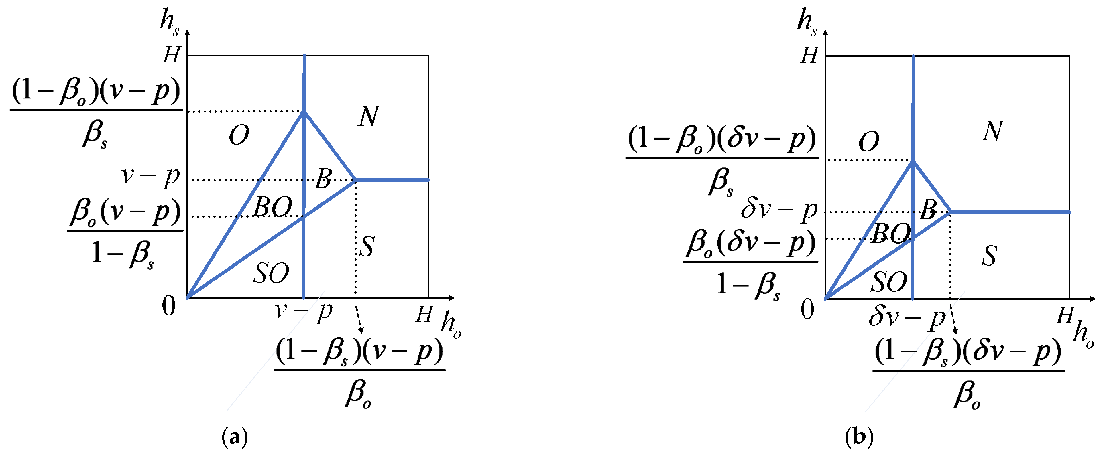
Figure 1. Market segmentation of H-type and L-type consumers when β o + β s 1 . (a) H-type consumers; (b) L-type consumers.
Axioms 12 00029 g001
Figure 2. Market segmentation of H-type and L-type consumers when β o + β s > 1 . (a) H-type consumers; (b) L-type consumers.
Axioms 12 00029 g002
Figure 3. Market segmentation of L-type consumers when coupons are offered and β o + β s 1 .
Axioms 12 00029 g003
Figure 4. Market segmentation of L-type consumers when coupons are offered and β o + β s > 1 . (a) f 2 < ( β o + β s 1 ) ( δ v p ) 1 β o ; (b)   f 2 ( β o + β s 1 ) ( δ v p ) 1 β o .
Axioms 12 00029 g004
Figure 5. Changes in the brand’s profit with f and q when β o = β s = 0.4 .
Axioms 12 00029 g005
Figure 6. Changes in the brand’s profit with f and q when β o = β s = 0.6 .
Axioms 12 00029 g006
Figure 7. Impacts of p and δ on the brand’s profit difference with different β o + β s . (a) β o = β s = 0.4 ; (b) β o = β s = 0.6 .
Axioms 12 00029 g007
Figure 8. Impacts of r on the brand’s profit with different β o + β s . (a) β o = β s = 0.4 ; (b) β o = β s = 0.6 .
Axioms 12 00029 g008
Figure 9. Impacts of p , δ , λ and r on coupon face value.
Axioms 12 00029 g009
Figure 10. Impacts of p , δ , λ and r on store inventory level. (a)   δ = 0.72 ,   λ = 0.8 ,   r = 0.2 ; (b) δ = 0.9 ,   λ = 0.8 ,   r = 0.2 ; (c)   δ = 0.72 ,   λ = 0.98 ,   r = 0.2 ; (d)   δ = 0.72 ,   λ = 0.8 ,   r = 0.5 .
Axioms 12 00029 g010
Figure 11. Impacts of p , δ , λ and r on the brand’s profit. (a) δ = 0.72 ,   λ = 0.8 ,   r = 0.2 ; (b) δ = 0.9 ,   λ = 0.8 ,   r = 0.2 ; (c) δ = 0.72 ,   λ = 0.98 ,   r = 0.2 ; (d) δ = 0.72 ,   λ = 0.8 ,   r = 0.5 .
Axioms 12 00029 g011
Table 1. Summary of symbols.
Parameters
v An H-type consumer’s valuation of the brand’s product
p Selling price of the product
λ Proportions of H-type consumers
δ Valuation coefficient of an L-type consumer for the product relative to an H-type consumer
c Unit cost of store inventory
r Unit cross-selling revenue for the brand
h o , h s , h b Hassle costs for consumers when they shop in the online, store and BOPS channels
Decision variables
f Coupon face value
q Store inventory level
Disclaimer/Publisher’s Note: The statements, opinions and data contained in all publications are solely those of the individual author(s) and contributor(s) and not of MDPI and/or the editor(s). MDPI and/or the editor(s) disclaim responsibility for any injury to people or property resulting from any ideas, methods, instructions or products referred to in the content.