Abstract
It is typically difficult to estimate the number of degrees of freedom due to the leptokurtic nature of the Student t-distribution. Particularly in studies with small sample sizes, special care is needed concerning prior choice in order to ensure that the analysis is not overly dominated by any prior distribution. In this article, popular priors used in the existing literature are examined by characterizing their distributional properties on an effective support where it is desirable to concentrate on most of the prior probability mass. Additionally, we suggest a log-normal prior as a viable prior option. We show that the Bayesian estimator based on a log-normal prior compares favorably to other Bayesian estimators based on the priors previously proposed via simulation studies and financial applications.
MSC:
62C10; 62F15; 62F10
1. Introduction
Student’s t-distribution [1] occurs frequently in statistics. Its usual derivation and utility is as the sampling distribution of certain test statistics derived based on normality [2]; however, over the past decades there has been growing interest in using the t-distribution as a heavy-tailed alternative to Gaussian distribution when robustness to possible outliers is a concern [3,4]. For example, it is widely known that the fluctuations in many financial time series are not normal [5,6]. As such, t-distribution is commonly used in finance and risk management, particularly to model asset or market index returns, for which the tails of the Gaussian distribution are almost invariably found to be too thin [7,8,9,10,11].
We assume that random variables are independently and identically distributed according to the Student t-distribution
depending on the number of degrees of freedom . Here, the notation denotes the parameter space , represents the gamma function, and the parameter controls the heaviness of the tails of the density, including particular cases of , where the distribution coincides with the Cauchy density, and , where the distribution converges to the standard normal density.
In this paper, the number of degrees of freedom in Student t-distributions is the parameter of main interest. If a reasonable range of the degrees of freedom is known, the value can be used as a tuning parameter in robust statistical modeling [4,12]. However, there is often very limited knowledge about the degrees of freedom , and it may be desirable to estimate based only on observed data that are believed to be independently sampled from the t-distribution (1). In particular, it is widely known that in small-sample studies the accurate estimation of the degrees of freedom is very difficult within both frequentist and Bayesian settings (see [3,13,14] and references therein).
In this paper, we re-examine a fully Bayesian way of estimating the number of degrees of freedom and suggest a new Bayesian estimator (i.e., posterior mean) based on a log-normal prior. To our knowledge, no previous research has studied log-normal distribution as a viable prior option in this context; hence, studying the operating characteristics of the Bayes estimator based on a log-normal prior compared to those of several existing Bayes estimators is of interest in its own right. There are ample examples of priors used in diverse applications for estimating the degrees of freedom [3,15,16,17]. Broadly, these priors fall into two classes according to whether they are (i) elicited from certain parametric distributions (e.g., exponential and gamma distributions) [15,16] or are (ii) constructed by formal rules such as the Jeffreys rule [3,18,19,20,21]. Despite certain differences in the derivation procedures between these two classes of priors, to a certain extent the motivation for using such priors is to have a robust Bayes estimator against outliers, possibly equipped with the appearance of objectivity in the statistical analysis [22,23], even when the sample size is fairly or moderately small, say, or 100.
This article is organized as follows. In Section 2, we formulate an inference problem for fully Bayesian estimation of the degrees of freedom, investigate a sufficient condition to induce a valid posterior inference, and introduce popular previously used prior distributions from the literature. Section 3 provides a state-of-the-art sampling algorithm to compute the Bayes estimator based on a log-normal prior. In Section 4, numerical experiments are conducted for the sensitivity analysis associated with the log-normal prior and for the comparison of the small-sample performance of several Bayes estimators. The performances of these Bayes estimators are further compared through a real data application in Section 5. Finally, Section 6 concludes the article.
2. Bayesian Inference
2.1. Validity of Estimation of the Degrees of Freedom
The Bayesian inference for the estimation of the number of degrees of freedom commences with specifying a prior density function supported on the parameter space , followed by evaluating the posterior density function
where represents the likelihood based on the t distribution (1). The denominator in (2), is called the marginal likelihood of observations . To have a valid posterior inference, the marginal likelihood should be finite for all . However, as the likelihood converges to a positive constant, as (more precisely, it holds uniformly for all where the represents the density of the N-dimensional multivariate standard normal distribution; see Equation (1.1) from [24]), the propriety of the posterior is highly dependent on the rate of decay of the prior . As such, it is nontrivial whether is finite when the likelihood is based on the distribution of t.
In the following, we show that when a prior is proper and supported on the parameter space , the posterior density is as well. To show this, we first prove that the two functional components of the distribution of t (1) are bounded on .
Lemma 1.
Consider functions and defined on the domain . Then, functions g and h are upper bounded on the domain .
Proof.
Using elementary calculus, we can show that the following three properties hold for the function : (i) g is continuous on ; (ii) ; and (iii) . Therefore, the function is upper bounded on the domain .
Next, we explore the three properties of the function on the domain . First, because the gamma function is continuous on the domain , the function on the domain is as well. Second, it holds that , because the nominator of h converges to the constant and the denominator of h diverges to , as goes to . That is, and . The latter is true due to a property of the gamma function, where is the Euler–Mascheroni constant and is the Riemann zeta function [25]. Finally, using Stirling’s approximation [26], that is, , with the nominator and denominator of , the following equality is obtained:
Because it generally holds that , we have . Thus, the function is upper bounded on the domain due to the three derived properties of the function. This ends the proof. □
Lemma 1 states that the likelihood function based on Student’s t-distribution, that is, the function of with a fixed x, (1), is bounded over the parameter space . Thus, we comment that the argument in [3] (“Unfortunately, the estimation of ν is not straightforward: the likelihood function tends to infinity as ”) is not correct. In actuality, the likelihood function tends to zero, as .
We can now prove the main theorem.
Theorem 1.
Suppose that is a random sample of size N from the distribution of t (1) with degrees of freedom . Let be a proper prior density supported on . Then, the posterior density is proper as well.
Proof.
Under the formulation of Bayes’s theorem where our eventual purpose is to prove that the marginal likelihood is finite for all values . By Lemma 1, there exists a constant C independent of such that
Because the prior density is proper (that is, ), the upper bound of the above inequality is finite. □
Here, we briefly summarize theoretical results before moving to the next subsection. Generally, in most Bayesian statistical inference, a proper prior can lead to a proper posterior, particularly when Gaussian likelihood (which has very light tails) is assumed. However, this may not be obvious when dealing with a likelihood function based on a fat-tailed distribution, such as Generalized Pareto distributions [27,28], Student’s t-distribution [1], -stable distribution [29], etc., that are frequently used in extreme value theory [30]. Theorem 1 states that a sufficient condition for a valid Bayesian inference in dealing with the t distribution is the propriety of the prior . On the other hand, for the case when the prior is improper, several authors [3,18,19] stated that the propriety of the posterior is generally not guaranteed. Unfortunately, there is no general theorem providing simple condition under which an improper prior yields the propriety of the posterior for a particular model, and as such this must be investigated on a case-by-case basis [31].
2.2. Effective Support of the Degrees of Freedom
Given data (1) with small sample sizes, the performance of a Bayesian estimator for heavily relies on the suitable allocation of the prior probability mass over the support . Ideally, the choice of prior is made such that most of the mass is placed on an interval that contains a range of plausible values for that can generate the data before observing the data. Such an interval, denoted as ‘’, is referred to as effective support of the degrees of freedom . The subscript ‘e’ in the notation is noted as emphasizing ‘effective’. Eventually, the prior probability on the effective support should be large enough to produce a Bayes estimator that performs well for .
Admittedly, a mathematical definition of the effective support in small-sample studies is not trivial, and may of course vary considerably for different values for observations and parameters (see the paper by [32] for a relevant theoretical discussion). Most works have used the interval as an effective support [3,18,19,33], although authors have used or as the effective support as well; throughout this paper, we use . One conventional reason behind this argument is that in a small-sample case the observations sampled from the t-distribution (1) with the degrees of freedom set by either , , or any other value greater than 25 can be virtually regarded as the observations from a standard normal distribution. To our knowledge, however, no research works have statistically justified the use of , or, similarly, or , as an effective support in the context of small-sample studies.
In this study, the Monte Carlo simulation method is used to examine the suitability of the interval for use as an effective support in small-sample cases. In general, Monte Carlo methods are widely used when the goal is to characterize certain statistical properties of a distribution under the finiteness of the sample size rather than resorting to a large-sample theory [34,35,36,37]. Experiments were designed as follows. With a choice from a list of sample size , we generated N observations , with the true data generating parameter selected from the interval . Here, at each value we simulated replication data instances of observations . From each instance of replication data, we calculated the p-value of the Shapiro–Wilk test [38] in order to evaluate the normality of the replication data. The null and alternative hypotheses at each value are thus as follows:
- •
- : a sample simulated from with the truth deriving from a normally distributed population;
- •
- : a sample simulated from with the truth does not derive from a normally distributed population.
Note that, under the above simulation setup, the source of the non-normality from the alternative hypothesis is mainly due to the heavy tails of observations t. Finally, we report the median value of the p-values obtained from the replication data at each true parameter .
Figure 1 displays the results of our experiments. Using the significance level as the criterion value (shown as the dashed horizontal line in the panel), we calculate a threshold value , dividing the interval into two sub-intervals, and . Then, the former interval comprises the parameters , generating heavy-tailed t observations, while the latter interval comprises the parameters , generating normal observations. Obviously, the threshold value is a function of the significance level and the sample size N; as such, it can be denoted as , although here we use to avoid cluttered notation. Conceptually, the threshold value may be interpreted as the transitional point at which the tail-thickness of N observations changes from heavy tails () to thin tails (), resulting in the threshold values are (), (), (), (), (), (), and ().

Figure 1.
Median of the p-values of the Shapiro–Wilk test from replicated observations with different sample size . The true data generating parameter is selected from the effective support .
The results of our Monte Carlo simulation experiments are summarized below:
- 1.
- As the sample size N increases from small sample sizes (i.e., ) to moderate sample sizes (i.e., ), the threshold value increases.
- 2.
- For the sample size (and similarly for , and 500, respectively), the values (and similarly for , and , respectively) generate the observations , which are virtually distributed in a normal distribution (with the type I error 0.05).
- 3.
- The interval effectively covers a wide range of tail-thickness, from heavy-tailed to thin-tailed data, up to the maximum sample size considered in the experiment. Thus, the interval can be used as an effective support for a small-sample study.
2.3. Prior Distributions for the Degrees of Freedom
Many prior distributions for the degrees of freedom suggested in the literature are proper distributions supported on the parameter space [18,39,40]. In Theorem 1, we have shown that this is a sufficient condition for a valid posterior inference. Examples of popularly used proper priors are based on an exponential distribution [15] and a gamma distribution [16]. On the other hand, a Jeffreys prior, as suggested by [3], is improper, yet it has been shown that the posterior under the Jeffreys prior is proper. In the linear regression setup, the Jeffreys prior is called the independence Jeffreys prior [18]. Readers may refer to the papers [3,15,16] for the formulation and derivation of the priors. Considering the effective support , as previously discussed, we aim to re-examine certain distributional properties of the three priors. Additionally, we study a log-normal distribution as a viable prior option. To the best of our knowledge, no previous study has reported the utility of a log-normal prior for robust Bayesian procedures. For the sake of readability, the four priors are denoted as (4), (5), (6), and (7), respectively, with the subsripts on the notations taken from the initials of the priors.
The following are the analytic expressions of the four priors:
- (a)
- Jeffreys prior [3]:where and are the digamma and trigamma functions, respectively. The authors of [3] developed the prior as an objective prior on the basis of certain Jeffreys rules [23]. The Jeffreys prior may place enormously substantial mass close to the zero due to the asymptotic behavior as ; see Corollary 1 from [3] for more details.
- (b)
- Exponential prior [15]:The specification of the rate hyperparameter as is recommended in [15] to avoid introducing strong prior information, for similar reasons as for using objective priors. The prior mean of equal to 10 and the prior variance of are equal to 100. Almost of the prior mass is allocated to the effective support , .
- (c)
- Gamma prior [16]:The authors of [16] recommend that the shape and rate hyperparameters be set to 2 and , respectively. Then, the prior mean and variance of are equal to 20 and 200, respectively. The gamma prior (6) allocates nearly of the prior mass to the effective support , .
- (d)
- Log-normal prior:We recommend setting the mean and variance hyperparameters to 1. These hyperparameters are specified on the basis of the sensitivity analysis in Section 4.1. The prior mean and variance of are and , respectively. The log-normal prior (7) places nearly of the prior mass on the effective support , .
Table 1 summarizes the first to second moments and mass allocation of the three prior densities (5), (6), and (7). As the Jeffreys prior is improper, we do not report it. Recall that in a small-sample study the transition from fat-tailed to normal-tailed t-distributed data is typically manifested on the effective interval (refer to Figure 1). Therefore, in order to achieve robust Bayesian procedures to dynamically accommodate data with a wide range of tail thicknesses, it is desirable that most of the probability of the prior mass is reasonably placed on the effective support . It is notable that the log-normal and exponential priors place substantial mass (98.6% and 91.7%) on the effective support, while the gamma prior places only 71.2% of the probability mass on the effective support. In Section 4.2, we conduct simulation studies to investigate the performances of Bayes estimators based on the priors.

Table 1.
Characteristics of prior densities on the interval .
3. Posterior Computation Using Log-Normal Priors
3.1. Elliptical Slice Sampler
In this section, we propose an efficient Markov chain Monte Carlo (MCMC) method to sample from the posterior density (2) when provided with the log-normal prior (7). Due to the non-conjugacy when sampling from the density , the first solution is to consider the Metropolis-Hastings (MH) algorithm [41,42], the performance of which can depend highly on the choice of the proposal density [43]. Instead, we can use the elliptical slice sampler (ESS) algorithm [44], which is known to be efficient when the prior distribution is a normal distribution. Conceptually, the MH and ESS algorithms are similar in that both comprise two steps, namely, a proposal step and a criterion step. A main difference between the two algorithms arises in the criterion step. If a new candidate does not pass the criterion, then the MH algorithm takes the current state as the next state, whereas the ESS re-proposes a new candidate until rejection does not take place, rendering the algorithm rejection-free. Unlike the MH algorithm, which requires the proposal variance or density, ESS is fully automated, and no tuning is required.
To adapt the ESS to simulate a Markov chain from the posterior density (2), we first need to transform to a real-valued parameter :
where . ESS can be used to sample from the transformed target density (8), after which the drawn sample should be transformed back to . Algorithm 1 details the ESS in an algorithmic form:
| Algorithm 1: ESS to sample from (2) |
Goal: Sampling from the full conditional posterior distribution
Input: Current state . Output: A new state .
|
In Algorithm 1, the logarithm of the ratio part in the criterion function can be detailed as follows:
To calculate the above quantity using R statistical software, the built-in function lgamma is recommended in order to produce stable calculation of the logarithm of the gamma function evaluated at , , , and .
3.2. Bayesestdft R Package
We developed an R package called bayesestdft to provide Bayesian tools to estimate the degrees of freedoms by sampling from the posterior distribution (2) with the likelihood , the log-normal prior , and hyperparameters with mean and variance . Note that with the specification we have (7). The function BayesLNP(y, ini.nu, S, mu, rho.sq) implements the ESS (Algorithm 1) with the following inputs:
- y: N-dimensional vector of continuous observations supported on , .
- ini.nu: the initial posterior sample value, (Default = 1).
- S: the number of posterior samples, S (Default = 1000).
- mu: mean of the log-normal prior density, (Default = 1).
- sigma.sq: variance of the log-normal prior density, (Default = 1).
The output of the function BayesLNP is the S-dimensional vector of posterior samples, that is, , and is drawn from the posterior density .
In order to demonstrate the estimation performance of the Bayes estimator based on the log-normal prior (7), we conducted the following simulation experiments. We generated observations with the truth value specified by and 5, respectively, and then estimated the parameter using the function BayesLNP for each of the three scenarios. To that end, we used the following command:
- R>
- library(devtools)
- R>
- devtools::installgithub("yain22/bayesestdft")
- R>
- library(bayesestdft)
- R>
- x1 = rt(n = 100, df = 0.1); x2 = rt(n = 100, df = 1); x3 = rt(n = 100, df = 5)
- R>
- nu.1 = BayesLNP(x1); nu.2 = BayesLNP(x2); nu.3 = BayesLNP(x3)
The outputs nu.1, nu.2, and nu.3 are number of posterior samples from each of the scenarios. Figure 2 displays the trace plots after burning the first hundred posterior samples. The results show that ESS (Algorithm 1) possesses a good mixing property and a reasonably high accuracy. More thorough simulation studies are described in Section 4.

Figure 2.
Trace plots for the three simulation experiments. Training data generated from Student t-distribution with (left), (middle), and (right).
The package bayesestdft includes a function BayesJeffreys to implement an MCMC algorithm to sample from the posterior distribution based on the Jeffreys prior (4). The sampling engines are a random walk Metropolis algorithm [45] and a Metropolis-adjusted Langevin algorithm (MALA) [46,47]. The relevant gradient calculation for implementing MALA is performed using the numDeriv R package; users can see the manual in help(BayesJeffreys) for more detail.
4. Numerical Studies
4.1. Sensitivity Analysis for a Log-Normal Prior
This subsection presents frequentist properties of Bayes estimators of the parameter based on a log-normal prior with four different choices of the hyperparameters . The purpose of this analysis is to measure the impact of the four log-normal priors on the posterior inference about and select the most promising hyperparameters out of the four choices, which are then coherently used in the subsequent analyses. As for performance metrics, we report the frequentist mean squared error (MSE) and the frequentist coverage of 95% credible intervals. These are widely used in assessing the accuracy of robust Bayesian procedures [3,19]. For the MSE, we report the median value of the MSEs based on 1000 replications.
The detailed simulation procedures are explained here. We considered drawing independent and identically distributed N samples from the student t-distribution (1) with the true data generating parameter specified from the effective support . After specifying a prior from the four prior options above (which only differ in the hyperparameters), we obtain the posterior mean and the credible interval () based on posterior samples . For the purpose of the stabilization to the stationary distribution, we draw samples from the posterior , followed by 500 burn-in and 10 thinning. As a result, for a single replicated data at each evaluation point , we can calculate the square root of the relative MSE and a coverage indicator , where if and 0 otherwise. In particular, the frequentist coverage of 95% credible interval (which is mathematically defined as ) can be approximated by taking the mean of the resulting values across the replications. A smaller value of the relative MSE indicates more accurate estimation. For the frequentist coverage of the 95% credible interval, a value closer to 0.95 indicates better coverage performance.
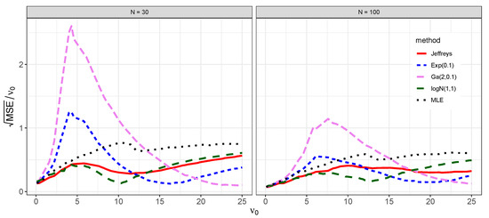
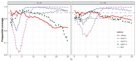
The results of the simulation are shown in Figure 3 and Figure 4. As expected, for all prior choices the relative MSEs are smaller for than for , and the coverage properties are closer to for than for across the values . For both and the performance of the posterior mean based on the standard log-normal prior is not good if is greater than 10. This is because the standard log-normal prior places too much mass on the interval , and hence the estimation performance deteriorates as becomes larger. Although the prior produces the best frequentist coverage with a 95% credible interval over the wide range of the effective support , its MSE is higher than those of other priors for () and (). The performance based on the priors and in terms of MSE is quite similar for , although the former performs better than the latter for on the values . Based on these results, we opted to use (7) as the default choice of the log-normal prior, as it produces reasonably stable estimation on the effective support compared to the other choices.

Figure 3.
Frequentist properties of the posterior mean based on the four log-normal priors with for sample sizes and . The y-axis value is the square root of the relative MSE and the x-axis value is the true data-generating parameter on the effective support .

Figure 4.
Frequentist coverage of credible intervals for the degrees of freedom based on the four log-normal priors with for sample sizes and . The horizontal dashed line represents target coverage.
The sensitivity analysis described in this section considered four choices of hyperparameters. While it would obviously be more desirable to select the hyperparameters from a larger number of options, the results show that our choice of produces reasonably accurate estimation compared to other priors in both numerical and real data studies.
4.2. Numerical Comparison Using the Jeffreys, Exponential, Gamma, and Log-Normal Priors
This subsection compares frequentist properties of posterior inference based on the four priors (4), (5), (6), and (7). The simulation designs are explained in Section 4.1. Additionally, we consider the maximum likelihood estimator (MLE) of to examine the performance of the frequentist approach compared to Bayesian approaches in estimating the parameter . For the MLE, in order to assess the coverage of confidence interval, we used a bootstrap confidence interval based on the MLE of [48], as the exact confidence interval was not available. For implementation, the functions BayesJeffreys and BayesLNP were used to obtain Bayes estimators for based on the priors (4) and (7), for which the sampling engines were ESS and MALA, respectively. To obtain Bayes estimators based on the priors (5) and (6), we used Stan [49], which uses a Hamiltonian Monte Carlo algorithm [50]. Finally, the MLE of was computed by using the function fitdistr(densfun = “t”) within library(MASS).
The results of the simulation are shown in Figure 5 and Figure 6. As expected, when using Bayesian and frequentist methods, the relative MSEs are smaller for than for across the values . For the Bayesian methods, the coverage properties tend to improve (that is, are closer to 0.95) for than for . In contrast, when using frequentist methods the coverage property becomes more conservative (that is, less than 0.95) for than for across the values . The Bayes estimator based on the Jeffreys prior (4) results in relatively lower MSE then the MLE over the values , in agreement with [3]. This is to some extent expected, as MLE can generally suffer in small-sample studies [51]. It is important to note that no Bayes estimator dominates other estimators over the entire interval . In other words, each Bayes estimator has its own region where the estimator is non-inferior to others.
The followings key points summarize the results of the simulations:
- (i)
- (ii)
- The Bayes estimator based on the log-normal prior (7) outperforms other estimators for () and ().
- (iii)
- The Bayes estimator based on the exponential prior (5) outperforms other estimators for () and ();
- (iv)
- The Bayes estimator based on the gamma prior (6) outperforms other estimators for () and ().
5. Real Data Analysis
To further assess the performance of the Bayes estimators based on the priors (4), (5), (6), and (7), we analyzed a sample of the daily index values from four countries: the United States (S&P500), Japan (NIKKEI225), Germany (DAX Index), and South Korea (KOSPI). In particular, we considered the data from 2 June 2009 to 30 October 2009, amounting to around 100 observations. The actual analysis was performed on the daily log-rate returns multiplied by 100, that is, , where is the market index on the i-th trading day. The transformed data for the period of interest are plotted in Figure 7. It can be seen that the series are stationary and that their variances can be reasonably considered as constant over the relevant period. The dataset used here can be loaded using data(index_return) in the R package bayesestdft.
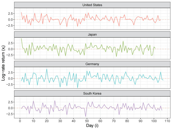
Figure 7.
Daily returns of the index values from four countries for the period spanning 6 May 2009 to 30 September 2009.
Table 2 lists the basic descriptive statistics of the index return series from the four countries. Note that the kurtosis is larger than 3 for every country, and even though the distribution of the returns does not have tails much heavier than a normal distribution it seems to be appropriate to consider a t model. Several researchers have found that Student’s t-distribution is the best marginal distribution for index returns [11,52]. Specifically, the model is , , with sample sizes (United States), 101 (Japan), 107 (Germany), and 106 (South Korea) and the goal of estimating the degrees of the freedom .
Table 2.
Descriptive statistics of the daily index returns.
The results of the posterior inference as summarized by posterior mean and 95% credible interval on the parameter are reported in Table 3. Additionally, in order to compare the model fit, we report the deviance information criterion (DIC) based on the posterior samples; see Equation (10) in [53] for the analytic formula of the DIC. A smaller value of DIC indicates better modeling fitting. The best inference result is in bold in the table from each country. It can be seen that the Bayes estimator based on the log-normal prior (7) performs the best for the series from the United States, Japan, and South Korea, while the Jeffreys prior (4) produces the best model fitting for the series from Germany.
Table 3.
Estimation results based on the four priors.
6. Concluding Remarks
In this paper, we studied three popular existing priors, namely, the Jeffreys [3], exponential [15], and gamma prior [16] distributions, and suggested a log-normal distribution as an alternative to produce accurate estimation for the number of degrees of freedom for Student’s t-distribution in a small-sample study. The Jeffreys prior has no hyperparameter. Estimation results based on the exponential and gamma priors can be sensitive to the choice of their hyperparameters, and we therefore set these values as the original authors suggested [15,16]. The use of a log-normal prior represents a new trial; hence, we performed a sensitivity analysis to select reasonable hyperparameters. The posterior computation algorithm used to calculate the Bayes estimator based on the log-normal prior possesses good operating characteristics in terms of balancing sampling and estimation accuracy without requiring expert-tuning. We were able to fairly compare the small-sample performance of the four priors through simulation studies for both an effective support and a real data application. The results show that the performance of the Bayes estimator based on the log-normal prior is reasonably good compared to the others. This elucidates the usefulness of the log-normal prior for more complex model settings such as linear regression, nonparametric regression, time-series analysis, and machine learning models, when t errors would be more desirable than using Gaussian errors to carry out robust Bayesian analyses [54].
Funding
This research received no external funding.
Data Availability Statement
Code is publicly available in developed R package bayesestdft. Visit Github repository (https://github.com/yain22/bayesestdft/tree/master/data, accessed on 22 July 2022) for the datasets analysed during the current study.
Conflicts of Interest
The author declares no conflict of interest.
References
- Student. The probable error of a mean. Biometrika 1908, 1–25. [Google Scholar]
- Casella, G.; Berger, R.L. Statistical Inference; Cengage Learning: Boston, MA, USA, 2021. [Google Scholar]
- Fonseca, T.C.; Ferreira, M.A.; Migon, H.S. Objective Bayesian analysis for the Student-t regression model. Biometrika 2008, 95, 325–333. [Google Scholar] [CrossRef]
- Lange, K.L.; Little, R.J.; Taylor, J.M. Robust statistical modeling using the t distribution. J. Am. Stat. Assoc. 1989, 84, 881–896. [Google Scholar] [CrossRef]
- Teichmoeller, J. A note on the distribution of stock price changes. J. Am. Stat. Assoc. 1971, 66, 282–284. [Google Scholar] [CrossRef]
- Nolan, J.P. Financial modeling with heavy-tailed stable distributions. Wiley Interdiscip. Rev. Comput. Stat. 2014, 6, 45–55. [Google Scholar] [CrossRef]
- Fernández, C.; Steel, M.F. Multivariate Student-t regression models: Pitfalls and inference. Biometrika 1999, 86, 153–167. [Google Scholar] [CrossRef]
- Zhu, D.; Galbraith, J.W. A generalized asymmetric Student-t distribution with application to financial econometrics. J. Econom. 2010, 157, 297–305. [Google Scholar] [CrossRef]
- Vrontos, I.D.; Dellaportas, P.; Politis, D.N. Full Bayesian inference for GARCH and EGARCH models. J. Bus. Econ. Stat. 2000, 18, 187–198. [Google Scholar]
- Bollerslev, T. A conditionally heteroskedastic time series model for speculative prices and rates of return. Rev. Econ. Stat. 1987, 542–547. [Google Scholar] [CrossRef]
- Hurst, S.R.; Platen, E. The marginal distributions of returns and volatility. Lect. Notes Monogr. Ser. 1997, 31, 301–314. [Google Scholar]
- West, M. Outlier models and prior distributions in Bayesian linear regression. J. R. Stat. Soc. Ser. 1984, 46, 431–439. [Google Scholar] [CrossRef]
- Liu, C.; Rubin, D.B. ML estimation of the t distribution using EM and its extensions, ECM and ECME. Stat. Sin. 1995, 5, 19–39. [Google Scholar]
- Villa, C.; Rubio, F.J. Objective priors for the number of degrees of freedom of a multivariate t distribution and the t-copula. Comput. Stat. Data Anal. 2018, 124, 197–219. [Google Scholar] [CrossRef]
- Fernández, C.; Steel, M.F. On Bayesian modeling of fat tails and skewness. J. Am. Stat. Assoc. 1998, 93, 359–371. [Google Scholar]
- Juárez, M.A.; Steel, M.F. Model-based clustering of non-Gaussian panel data based on skew-t distributions. J. Bus. Econ. Stat. 2010, 28, 52–66. [Google Scholar] [CrossRef]
- Jacquier, E.; Polson, N.G.; Rossi, P.E. Bayesian analysis of stochastic volatility models with fat-tails and correlated errors. J. Econom. 2004, 122, 185–212. [Google Scholar] [CrossRef]
- He, D.; Sun, D.; He, L. Objective Bayesian analysis for the Student-t linear regression. Bayesian Anal. 2021, 16, 129–145. [Google Scholar] [CrossRef]
- Villa, C.; Walker, S.G. Objective prior for the number of degrees of freedom of at distribution. Bayesian Anal. 2014, 9, 197–220. [Google Scholar] [CrossRef]
- Jeffreys, H. Theory of Probability; Oxford University Press: New York, NY, USA, 1961; p. 472. [Google Scholar]
- Kass, R.E.; Wasserman, L. The selection of prior distributions by formal rules. J. Am. Stat. Assoc. 1996, 91, 1343–1370. [Google Scholar] [CrossRef]
- Berger, J. The case for objective Bayesian analysis. Bayesian Anal. 2006, 1, 385–402. [Google Scholar] [CrossRef]
- Consonni, G.; Fouskakis, D.; Liseo, B.; Ntzoufras, I. Prior distributions for objective Bayesian analysis. Bayesian Anal. 2018, 13, 627–679. [Google Scholar] [CrossRef]
- Finner, H.; Dickhaus, T.; Roters, M. Asymptotic tail properties of Student’s t-distribution. Commun. Stat. Methods 2008, 37, 175–179. [Google Scholar] [CrossRef]
- Abramowitz, M.; Stegun, I.A.; Romer, R.H. Handbook of Mathematical Functions with Formulas, Graphs, and Mathematical Tables; USA Department of Commerce: Washington, DC, USA, 1988.
- Jameson, G.J. A simple proof of Stirling’s formula for the gamma function. Math. Gaz. 2015, 99, 68–74. [Google Scholar] [CrossRef][Green Version]
- Lee, S.; Kim, J.H. Exponentiated generalized Pareto distribution: Properties and applications towards extreme value theory. Commun. Stat. Theory Methods 2019, 48, 2014–2038. [Google Scholar] [CrossRef]
- Castillo, E.; Hadi, A.S. Fitting the generalized Pareto distribution to data. J. Am. Stat. Assoc. 1997, 92, 1609–1620. [Google Scholar] [CrossRef]
- DuMouchel, W.H. On the asymptotic normality of the maximum-likelihood estimate when sampling from a stable distribution. Ann. Stat. 1973, 1, 948–957. [Google Scholar] [CrossRef]
- De Haan, L.; Ferreira, A.; Ferreira, A. Extreme Value Theory: An Introduction; Springer: Berlin/Heidelberg, Germany, 2006; Volume 21. [Google Scholar]
- Northrop, P.J.; Attalides, N. Posterior propriety in Bayesian extreme value analyses using reference priors. Stat. Sin. 2016, 26, 721–743. [Google Scholar] [CrossRef]
- Chu, J. Errors in Normal Approximations to the t, tau, and Similar Types of Distribution. Ann. Math. Stat. 1956, 27, 780–789. [Google Scholar] [CrossRef]
- Wang, M.; Yang, M. Posterior property of Student-t linear regression model using objective priors. Stat. Probab. Lett. 2016, 113, 23–29. [Google Scholar] [CrossRef]
- Metropolis, N.; Ulam, S. The monte carlo method. J. Am. Stat. Assoc. 1949, 44, 335–341. [Google Scholar] [CrossRef] [PubMed]
- Thomas, D.R.; Rao, J. Small-sample comparisons of level and power for simple goodness-of-fit statistics under cluster sampling. J. Am. Stat. Assoc. 1987, 82, 630–636. [Google Scholar] [CrossRef]
- Razali, N.M.; Wah, Y.B. Power comparisons of shapiro-wilk, kolmogorov-smirnov, lilliefors and anderson-darling tests. J. Stat. Model. Anal. 2011, 2, 21–33. [Google Scholar]
- Massey, F.J., Jr. The Kolmogorov-Smirnov test for goodness of fit. J. Am. Stat. Assoc. 1951, 46, 68–78. [Google Scholar] [CrossRef]
- Shaphiro, S.; Wilk, M. An analysis of variance test for normality. Biometrika 1965, 52, 591–611. [Google Scholar] [CrossRef]
- Ho, K.W. The use of Jeffreys priors for the Student-t distribution. J. Stat. Comput. Simul. 2012, 82, 1015–1021. [Google Scholar] [CrossRef]
- Geweke, J. Bayesian treatment of the independent Student-t linear model. J. Appl. Econom. 1993, 8, S19–S40. [Google Scholar] [CrossRef]
- Hastings, W.K. Monte Carlo sampling methods using Markov chains and their applications. Biometrika 1970, 57, 97–109. [Google Scholar] [CrossRef]
- Metropolis, N.; Rosenbluth, A.W.; Rosenbluth, M.N.; Teller, A.H.; Teller, E. Equation of state calculations by fast computing machines. J. Chem. Phys. 1953, 21, 1087–1092. [Google Scholar] [CrossRef]
- Chib, S.; Greenberg, E. Understanding the metropolis-hastings algorithm. Am. Stat. 1995, 49, 327–335. [Google Scholar]
- Murray, I.; Prescott Adams, R.; MacKay, D.J. Elliptical slice sampling. arXiv 2010, arXiv:1001.0175. [Google Scholar]
- Gustafson, P. A guided walk Metropolis algorithm. Stat. Comput. 1998, 8, 357–364. [Google Scholar] [CrossRef]
- Ma, Y.A.; Chen, Y.; Jin, C.; Flammarion, N.; Jordan, M.I. Sampling can be faster than optimization. Proc. Natl. Acad. Sci. USA 2019, 116, 20881–20885. [Google Scholar] [CrossRef]
- Dwivedi, R.; Chen, Y.; Wainwright, M.J.; Yu, B. Log-concave sampling: Metropolis-Hastings algorithms are fast! In Proceedings of the Conference on Learning Theory (PMLR), Stockholm, Sweden, 6–9 July 2018; pp. 793–797. [Google Scholar]
- Efron, B. Bootstrap methods: Another look at the jackknife. In Breakthroughs in Statistics; Springer: Berlin/Heidelberg, Germany, 1992; pp. 569–593. [Google Scholar]
- Stan Development Team. RStan: The R Interface to Stan, R Package version; Stan Development Team, 2016; Volume 2, p. 522. Available online: https://mc-stan.org (accessed on 22 July 2022).
- Hoffman, M.D.; Gelman, A. The No-U-Turn sampler: Adaptively setting path lengths in Hamiltonian Monte Carlo. J. Mach. Learn. Res. 2014, 15, 1593–1623. [Google Scholar]
- Van de Schoot, R.; Kaplan, D.; Denissen, J.; Asendorpf, J.B.; Neyer, F.J.; Van Aken, M.A. A gentle introduction to Bayesian analysis: Applications to developmental research. Child Dev. 2014, 85, 842–860. [Google Scholar] [CrossRef]
- Praetz, P.D. The distribution of share price changes. J. Bus. 1972, 45, 49–55. [Google Scholar] [CrossRef]
- Gelman, A.; Hwang, J.; Vehtari, A. Understanding predictive information criteria for Bayesian models. Stat. Comput. 2014, 24, 997–1016. [Google Scholar] [CrossRef]
- Berger, J.O.; Moreno, E.; Pericchi, L.R.; Bayarri, M.J.; Bernardo, J.M.; Cano, J.A.; De la Horra, J.; Martín, J.; Ríos-Insúa, D.; Betrò, B.; et al. An overview of robust Bayesian analysis. Test 1994, 3, 5–124. [Google Scholar] [CrossRef]
Publisher’s Note: MDPI stays neutral with regard to jurisdictional claims in published maps and institutional affiliations. |
© 2022 by the author. Licensee MDPI, Basel, Switzerland. This article is an open access article distributed under the terms and conditions of the Creative Commons Attribution (CC BY) license (https://creativecommons.org/licenses/by/4.0/).