Article

Machine Learning-Based Modelling and Meta-Heuristic-Based Optimization of Specific Tool Wear and Surface Roughness in the Milling Process

by
Siamak Pedrammehr
1,2,*,
Mahsa Hejazian
3,
Mohammad Reza Chalak Qazani
2,
Hadi Parvaz
4,
Sajjad Pakzad
1,
Mir Mohammad Ettefagh
3 and
Adeel H. Suhail
5
1
Faculty of Design, Tabriz Islamic Art University, Tabriz 5164736931, Iran
2
Institute for Intelligent Systems Research and Innovation, Deakin University, Waurn Ponds, VIC 3216, Australia
3
Faculty of Mechanical Engineering, University of Tabriz, Tabriz 5166616471, Iran
4
Faculty of Mechanical and Mechatronics Engineering, Shahrood University of Technology, Shahrood 36199-95161, Iran
5
Department of Mechanical Engineering, Middle East College, PB 79, Al Rusayl, Muscat PC 124, Oman
*
Author to whom correspondence should be addressed.
Axioms 2022, 11(9), 430; https://doi.org/10.3390/axioms11090430
Submission received: 9 August 2022 / Revised: 21 August 2022 / Accepted: 22 August 2022 / Published: 26 August 2022
(This article belongs to the Special Issue Statistical Methods and Applications)

Abstract

:
The purpose of this research is to investigate different milling parameters for optimization to achieve the maximum rate of material removal with the minimum tool wear and surface roughness. In this study, a tool wear factor is specified to investigate tool wear parameters and the amount of material removed during machining, simultaneously. The second output parameter is surface roughness. The DOE technique is used to design the experiments and applied to the milling machine. The practical data is used to develop different mathematical models. In addition, a single-objective genetic algorithm (GA) is applied to numerate the optimal hyperparameters of the proposed adaptive network-based fuzzy inference system (ANFIS) to achieve the best possible efficiency. Afterwards, the multi-objective GA is employed to extract the optimum cutting parameters to reach the specified tool wear and the least surface roughness. The proposed method is developed under MATLAB using the practically extracted dataset and neural network. The optimization results revealed that optimum values for feed rate, cutting speed, and depth of cut vary from 252.6 to 256.9 (m/min), 0.1005 to 0.1431 (mm/rev tooth), and from 1.2735 to 1.3108 (mm), respectively.

1. Introduction

The estimation of tool life is an important area of research in the field of material machining. In order to maximize tool life, the right set of parameters must be used to optimize and better use the cutting tool and machining process. The capacity of the cutting tools is being improved and is the subject of intensive study. The main goal of this experimental research is to investigate how the milling operation’s cutting conditions—such as cutting depth, speed, and feed—affect tool wear.
The replacement of tools, which is a result of tool wear, is one of the most significant economic components of machining. The productivity of the process is often immediately impacted by a reduction in the material removal rate as the tool wear criteria decline. Surface roughness, on the other hand, must also be taken into account as a quality attribute of the machined surface. There are many different optimization techniques available to solve engineering problems such as this. Many academics in the past focused more on the machining process and paid less attention to milling operations, basing their studies on modeling, tool wear, and surface roughness. Additionally, they did not assess their optimization strategy against those of other scholars.
A hybrid optimization approach was employed by Yildiz et al. [1]. There were comparisons made between their findings and those of other researchers to indicate that their strategy was effective in improving process parameters during machine operations using the Nelder–Mead local search algorithm and the optimization algorithm of Harris Hawks. In a separate study, they optimized the processing parameters for several industrial processes using the multi-verse, grasshopper, and Harris Hawks optimization algorithms [2]. Savkovic et al. [3] constructed trustworthy intelligent models for selecting the milling process’s output features based on the machining process’s input parameters. The ideal mixture of process factors for optimal response—surface roughness, material removal rate, and strength—was chosen by Khawaja et al. [4] after considering mathematical models and using the response surface approach. Chien and Tsai [5] also created a model for forecasting tool flank wear using the modeling approach. They then used a genetic algorithm to improve the model to identify the ideal cutting conditions for the machining of 17-4PH stainless steel. By looking into flank wear and surface roughness while turning an Al/SiCp metal matrix composite, Sahoo and Pradhan [6] looked into the machining properties. They used the Taguchi technique to do this. The outcome of their research demonstrates that adhesion and abrasion are the most frequent wear processes. The Taguchi approach was also used by Mia et al. [7]. Their experiment was designed using a Taguchi orthogonal array and a signal-to-noise ratio optimization method. They used coated carbide tools for rough machining and MQL to assess the tool’s wear characteristics and surface roughness. The findings indicate that although cutting depth affects tool wear, cutting speed substantially impacts surface roughness. Tsao [8] further used the Taguchi approach to enhance milling process parameters. Based on the findings, the flank wear was reduced by 62 percent using the suggested strategy. A distinct approach is used by Amouzgar et al. [9] to optimize the depth of tool wear. They used evolutionary algorithms to reduce tool wear and the interface temperature after simulating a turning operation using the finite element approach first. Seventy percent of the calculation time was shaved off. Aluminum alloy 7075 was the choice of Savkovi et al. [10], who looked at how cutting forces and factors affected surface roughness during milling. As a consequence of their research, the cutting force was shown to be ideal when the surface area was kept to a minimum for all input values. Additionally, the best alternatives for creating moderate computational roughness were minimal values for cutting speed, feed per tooth, cutting depth, and average level.
Recently, deep learning and machine learning techniques have been developed and have gained a remarkable interest across different research fields such as materials, microstructure, manufacturing, and energy [11,12,13]. The data-driven modeling methods are not based on the physics of process, and they often have a higher accuracy in comparison with the classical models [14]. Jia et al. [15] employed the particle swarm optimization method to obtain the optimum parameters for the production of mechanical materials. Pilania et al. [16] made materials property prediction using kernel ridge regression. Hwang et al. [17] proposed a four-layer perceptron for the rolled steel bar mechanical properties. Chen and Gu [18] reviewed the implemented machine learning techniques in composite material modelling and designing, and the mechanical properties of cold-rolled strip have been investigated through the feedforward neural network by Lalam et al. [19]. The developed model predicts the yielding strength and ultimate tensile strength with ±10 (MPa) accuracy for 90 percent of the data. Xiong et al. [20] investigated the estimation of the steels mechanical properties using four machine learning methods including random forest, linear least-square, k-nearest neighbors, and multilayer perceptron. Xie et al. [21] employed machine learning method to develop the mechanical properties online prediction for the hot rolled steel plate. Rajesh et al. [22] studied machine learning methods that have been used in manufacturing processes. In addition, machine learning methods have been applied to optimize different milling parameters such as tool condition monitoring [23,24], chatter detection and stability [25,26], prediction of cutting forces and power [27,28], and surface prediction [29,30].
In this research, the specific tool wear is introduced as a new output parameter named in which the material removal rate and tool wear are evaluated. The second target output is surface roughness. In order to reduce tool wear, increase surface smoothness, and increase the rate of material removal in an AISI 1045 alloy steel mill, three alternative optimization techniques have been put forward and contrasted. The main contribution of this research is to extract the optimal milling process parameters, including cutting speed (m/min), feed rate (mm/rev⸱tooth), and depth of cut (mm), in order to reach the optimal specific tool wear (mm) and surface roughness (cm/(cm3/s)) using multi-objective GA. It should be noted that higher specific tool wear means lower surface roughness, and there is a need of Pareto front to extract the optimal solutions of the milling process. In addition, the multi-objective functions of the milling process are extracted using adaptive network-based fuzzy inference system (ANFIS) to imitate the process based on the results of experiment. The optimal solutions are recommended at the end of this study.

2. Materials and Methods

The initial step in the investigation was to choose a subject matter for study. The intended piece of work was constructed using AISI 1045 alloy steel blocks (example dimensions: 150 × 80 × 60 (mm)). The tensile strength of this steel ranges from 570 to 700 (MPa), with low strain hardenability. In many different industries, axles, pins, belts, gears, pumps, and shafts are made from this normalized and softened alloy, which has a hardness range of 170 to 210 (HRC). A universal milling machine called the FP4MD was used for the experiments. With a spin speed range of 50 to 2500 (rpm) and a desk feed rate range of 0 to 900 (mm/min), this machine provides a positioning precision of +/−0.005 (mm). A 4-fluted face milling cutter, 80 (mm) in diameter, was utilized in the milling operation. An insert made of cemented carbide that was covered with TiN made up the cutting tool (ISO R245-12 T3 M-PM 4020). This insert may be used in semi-dry or dry machining operations because of the thermal shock resilience of the substrate and the PVD coating. The inserts utilized in the studies had a 13.4 (mm) engraved circular diameter, a 10 (mm) effective cutting-edge length, and a 1.5 (mm) corner radius.
This paper aims to extract the optimal block cutting parameters in progress to reach the optimum parameters of the process with the fewer testing trials (best surface roughness using less cutting force). One of the accurate machine learning techniques (ANFIS) was employed to extract the model to connect the cutting parameters to surface roughness and milling force. The hyperparameters of ANFIS were extracted using GA to reach the highest performance of the developed model. In this study, there were 2 different outputs (surface roughness and tool wear) for a dataset. The model was trained ten times to extract the optimal ANFIS model. The recorded tool wear factor and surface roughness were considered to develop the ANFIS model.
Figure 1 illustrates the scheme of the developed method in the current study as the main contribution, which combines ANFIS and the GA. According to Figure 1a, the process is started by selecting the appropriate cutting parameters. The surface quality was then evaluated using a roughness meter produced by the Taylor Habson firm after the FP4MD universal milling machine was finished. The Olympus company’s BX60 optical microscope, which has a 50× to 1000× magnification range, was also used.
The proposed algorithm includes the data pre-processing for eliminating the out-of-range data to enhance the accuracy of the algorithm. The single-objective GA was applied to choose the optimum ANFIS hyperparameters to achieve the least mean square error (MSE) between the predicted and actual data as it is shown in the left dashed line rectangular of Figure 1b.
The algorithm as initiated twice to extract ANFIS1 and ANFIS2 models to calculate the workpiece’s tool wear and surface roughness, as shown in the right dashed-line rectangle of Figure 1b, respectively. Then, the multi-objective GA as employed to extract the optimal cutting parameters of block in progress order to reach the most appropriate outcomes, including the specific tool wear and low surface roughness.
The proposed algorithm includes the data pre-processing for eliminating the out-of-range data to enhance the accuracy of the algorithm. The single-objective GA was applied to choose the optimum ANFIS hyperparameters to achieve the least mean square error (MSE) between the predicted and actual data as it is shown in the left dashed-line rectangle of Figure 1b.
The algorithm was initiated twice to extract ANFIS1 and ANFIS2 models to calculate the workpiece’s tool wear and surface roughness as shown in the right dashed-line rectangle of Figure 1b, respectively. Then, the multi-objective GA was employed to extract the optimal cutting parameters of block in progress order to reach the most appropriate outcomes, including the specific tool wear and low surface roughness.
Three variables: cutting speed, feed rate, and depth of cut, were considered in this research. Here, as the processes are time-consuming and expensive, out of 9 combinations, each with three replications, instead of 27 tests (full factorial) replications, the experiment was performed randomly by the Taguchi method (L9).

3. Mathematical Modelling

The goal of a mathematical model is to build an input–output connection to explain how the dependent variable’s usual value varies when each independent variable is changed. Furthermore, that is the initial stage to enable process optimization, the best milling settings to achieve the best possible surface smoothness, and particular tool wear. Table 1 displays the results of nine tests based on the Taguchi L9 matrix.
According to the breakdown, the first three columns represent independent cutting parameters. In contrast, the fourth and fifth columns represent dependent and objective outputs representing surface roughness and tool wear.

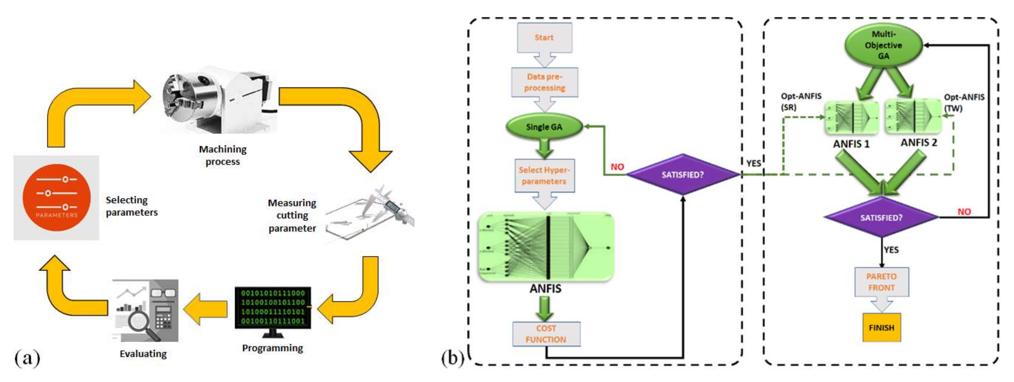
4. Optimization Procedure

Many real-world situations need the adjustment of process parameters to achieve desired results. A multi-target optimization issue aims to reduce two targets (responses) concurrently. As a result, one aim is often reduced while another is boosted in certain situations, which may lead to conflicting outcomes. If we want to find an acceptable solution that meets all of our goals while being as cost-effective as possible, we must use a trade-off approach. Tool wear during milling and workpiece surface roughness may be predicted using ANFIS, employed in this article to model these two variables.

4.1. Pre-Tuning of Algorithm

Three tasks need to be completed before creating the model and using the data. There are some statistics with a negative force at first. Since these data were produced as a result of the system’s dysfunction, they ought to be deleted. Before using the data inside the models, the out-of-range data caused by a sensor malfunction should also be eliminated. In order to simplify the data for a system before training, the second stage involves normalizing or standardizing the procedure. Both approaches are used in this work to reduce the complexity of the network’s input data and boost system accuracy. The standardization of the data is determined using the formula shown below:
σ x i = x i x ¯ σ x
where xi and σxi are, respectively, the raw and standardized ith inputs. σx and x ¯ are also the functions to extract the standard and average deviations of the data. The normalized data is calculated as:
n x i = x i x _ x ¯ x _

4.2. Adaptive Network-Based Fuzzy Inference System

ANFIS is a hybrid system made up of an artificial neural network and a fuzzy inference system that is utilized as a kind of Takagi–Sugeno artificial intelligence model to resolve nonlinear and challenging situations (FIS). This suggests that ANFIS has the capacity for both self-learning and logical operation. The following are the ANFIS fuzzy rules:
  • Rule 1: if t = O1, and x = P1:  z1 = a1t + a2x + a3.
  • Rule 2: if t = O2, and x = P2:  z2 = b1t + b2x + b3.
In which x and t are inputs, z1 and z2 are the outputs specified by the mentioned rules. During the learning process, the parameters a1, a2, a3, b1, b2, and b3 are acquired.
The ANFIS structure shown in Figure 2 has five levels, each with an output and two inputs, as shown. Layers of meaning are as follows:
In the first layer, membership functions are used to compute fuzzy clusters based on the training data input. The membership function is created using the indices ai and bi, and the degree of membership is calculated as follows:
Q i 1 = μ A i x = 1 1 + x c a 2 b ; i = 1 , 2
Q i 1 = μ B i x ; i = 1 , 2
where µx and µy are the degrees of membership. Ai and Bi are fuzzy sets and Q i 1 is the ith node in the jth layer output for input x.
Layer 2 is the rule that is applied to double the firing power. The output can be obtained as:
Q i 2 = w i = μ A i x · μ B i y ,   i = 1 , 2
Layer 3 used to normalize the firing intensity of the last layer. Dividing the ith rule’s firing strength by the sum of all firing strengths, the normalized values can be obtained as:
Q i 3 = w ¯ i = w i w 1 + w 2 + w 3 + w 4 ,   i = 1 , ,   4
The defuzzification layer is the fourth layer. The result can be obtained by the dot product of the parameters set (pi, qi, and ri) and the normalized firing strength, which yields:
Q i 4 = w ¯ i f i = w ¯ i p i x + q i y + r i
Adding each rule’s defuzzification outputs creates the final result of layer five:
Q i 5 = i w ¯ i f i = i w i f i i w i
Considering the backpropagation algorithm of the gradient descent method, the error signals can be obtained. This algorithm minimizes the training error by adjusting the customizable parameters.

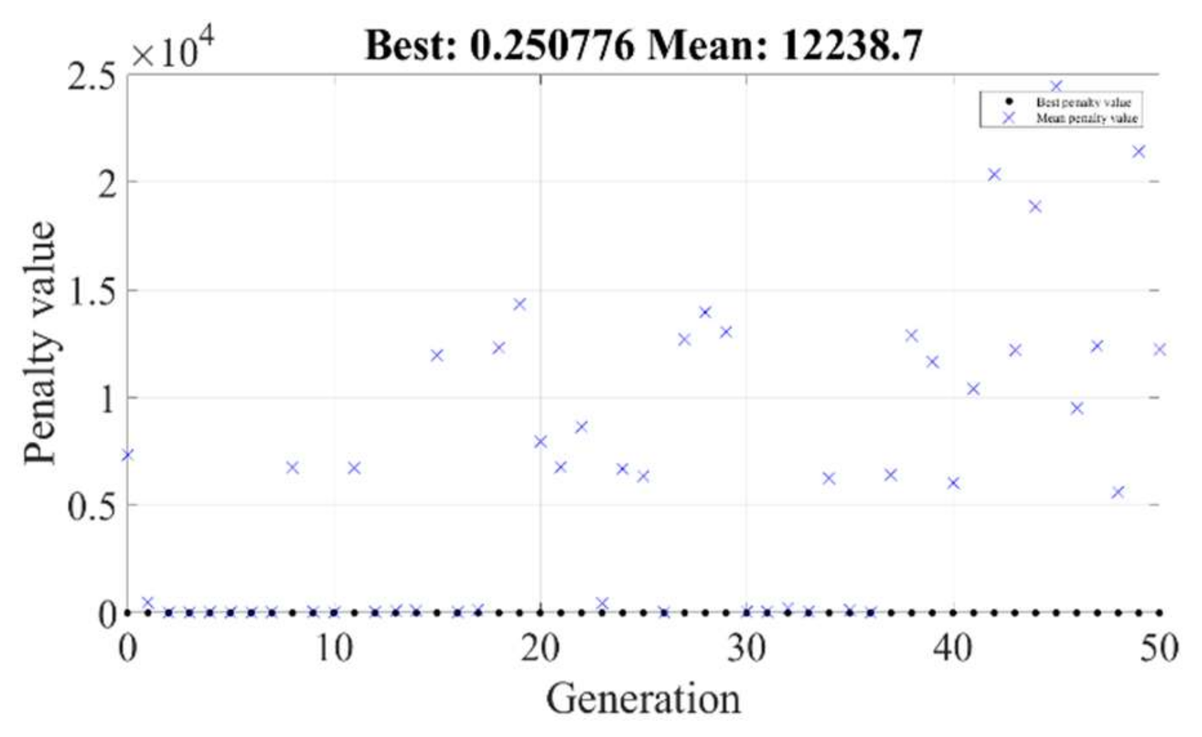
4.3. Genetic Algorithm

The GA belongs to the meta-heuristic algorithm classification of evolutionary-based algorithms, which solve the problem with and without being constrained. It is based on the natural selection of the evolutionary algorithms. Various optimization problems have led to the use of GA. It is a bio-inspired operator that makes use of mutation, crossover, as well as preference. Holland [25] suggested this technique depending on the natural selection procedure. Generating a randomly generated population of chromosomes is commonly the first stage in GAs. The fitness function is used to evaluate the extracted chromosomes. The chromosomes with a best approximation of optimal solution have a higher probability of reproducing. The GA parameters have a direct affect in the speed and the accuracy of the system regarding the appropriate convergence of the results. The appropriate crossover and mutation parameters guarantee the success rate of the GA [25]. The solution can be missed using a high mutation rate, which is close to the present state. On the other hand, the lower mutation rate can stick the process toward the local optimum. Furthermore, crossover prohibits offspring from being generated within the new generation; as a result, it will not be an identical replica of their parents’ previous population. The mutation index was set to a fair value and the crossover parameter to a more significant value, as De Jong and Michelle also tried [26]. The GA-based method for fixture layout’s machining was performed as: initialization of GA control parameters, fitness evaluation, new population (crossover, reproduction, mutation), and assessing the new population and termination criteria [27]. The GA results show that the crossover, mutation, generation, and population parameters have all been selected appropriately.
The right definition of the cost function is extremely important in optimization in order to reach highest possible system efficiency. In our study, the cost function is defined as follows:
J (t1, t2, t3) = 104 × MSE(Actual − Predicted)
where t1, t2, and t3 are the cutting parameters including feed rate, cutting speed, and depth of cut, respectively. Actual and predicted are the specific tool wear or surface roughness captured via the experimental or calculated result via the machine learning method.

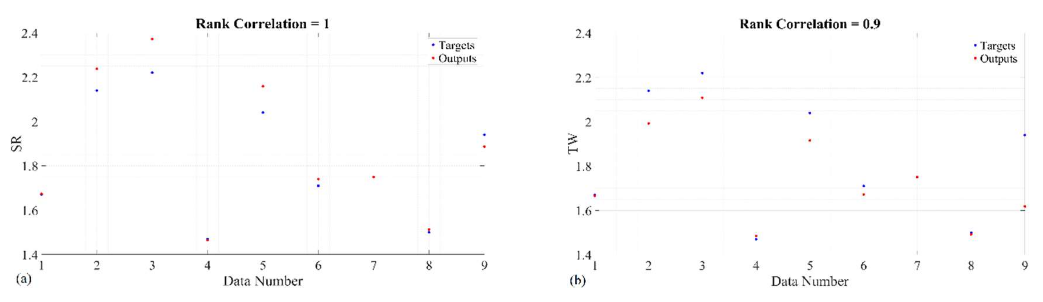
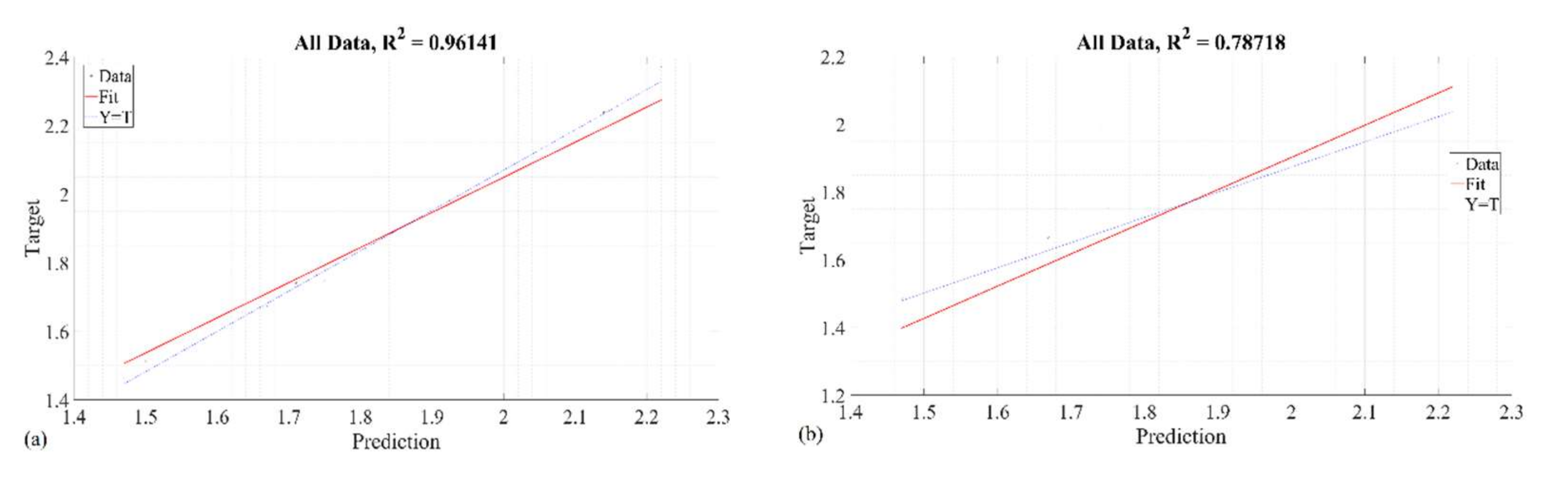
5. Results and Discussions

In this research, machining parameters have been modelled for the calculation of the tool wear and surface roughness based on the cutting parameters in the milling process. Then, the multi-objective GA function of MATLAB was used to extract the optimal cutting parameters of the process.
The MATLAB model used in Section 3’s GA optimization approach was created. The model provided in Section 4.2 is used to propose ANFIS. The model is then fine-tuned using the GA optimization approach described in Section 4.3.
MATLAB’s “ANFIS function” was employed to create the ANFIS simulation model. All of the findings in the Section 3 are illustrated using the “plot” function of MATLAB, which was used to create the algorithms. In addition, MATLAB’s “ga” and “gamultiobj” functions were used to create the GA and multi-objective GA, respectively. The proposed ANFIS, comprising ANFIS-TW and ANFIS-SR, has optimum hyperparameters that may be extracted using the single-objective GA optimization approach. The suggested ANFIS-SR and ANFIS-TW optimized hyperparameters for the milling process to forecast tool wear and surface roughness are shown in Table 2.
Figure 3 shows the optimization process of single-objective GA in the calculation of the optimum hyperparameters of the ANFIS-SR for maximum generation of 50. As is shown in Figure 3, the optimization is terminated after 44 generations as there was not any changed in the best value, which is the RMSE between the actual and predicted surface roughness via the ANFIS model. The extracted optimal hyperparameters are reported in the second row of Table 2. The employed cost function inside the single objective GA is based on Equation (9).
Figure 4 shows the optimization process of single-objective GA in calculation of the optimized hyperparameters of the ANFIS-TW for maximum generation of 50. As is shown in Figure 4, the optimization is not terminated during the 50th generation. The extracted optimal hyperparameters are reported in the third row of Table 2. The employed cost function inside the single objective GA is based on Equation (9).
Figure 5 shows the actual and predicted value of the specific tool wear and surface roughness. Seven datasets were chosen for training (78%), and two for the developed models testing (22%). According to the results illustrated in Figure 5a, it is quite apparent that ANFIS-SR predictions are more accurate compared to the ANFIS-TW during the testing and training procedures for the algorithms. It should be noted that the RMSE between the actual and predicted surface roughness of the milling process using the experimental setup and ANFIS-SR was 8.2086 × 10⁻¹⁶ (mm) based on Figure 5a. In addition, Figure 5b shows that the RMSE between the experimentally captured and predicted via ANFIS-TW of specific tool wear was 1.0649 × 10⁻¹⁵ (cm/(cm3/s)). In addition, the MSE between the predicted and actual surface roughness and specific tool wear using the experiment, ANFIS-SR, and ANFIS-TW were 6.7382 × 10⁻³¹ (mm) and 1.134 × 10⁻³⁰ (cm/(cm3/s)) based on Figure 5, respectively.
The t-test was carried out between the target and output values of surface roughness. The two-tailed p value was equal to 0.9323. By conventional criteria, this difference is considered to be not statistically significant. In addition, the standard error of difference is 0.135. Additionally, the t-test has been carried out between the target and output values of tool wear. The two-tailed P value was equal to 0.9167. The mean of Group One minus Group Two was equal to −0.000322. There was a 95% confidence interval of this difference (from −0.006747 to 0.006103). The standard error of difference equaled 0.003.
Figure 6 shows the histogram of error for the predicted data during the models’ testing and training procedures, including ANFIS-SR and ANFIS-TW. The error histogram of ANFIS-SR is right-skewed according to Figure 6a.
It has a smaller range of error that is between −0.2 and 0.1 (mm). In addition, the error histogram for ANFIS-TW is left-skewed in the range of −0.2 to 0.4 (cm/(cm3/s)). The average errors between the predicted and actual surface roughness using ANFIS-SR and specific tool wear ANFIS-TW were −3.9461 × 10⁻² (mm) and 8.187 × 10⁻² (cm/(cm3/s)), respectively. In addition, the variation of error histogram using ANFIS-SR and ANFIS-TW were 6.7689 × 10⁻² (mm) and 1.0849 × 10⁻¹ (cm/(cm3/s)), respectively.
The regression of the developed two methods, including ANFIS-SR and ANFIS-TW for whole data (i.e., testing and training), are, respectively, presented in Figure 7. ANFIS-SR and ANFIS-TW during training and testing were 0.96141 and 0.78718, respectively.
Based on a paired configuration of the inputs and outputs of ANFIS-SR, Figure 8 displays the derived fuzzy rule surface. Figure 8a depicts the effect of feed rate and cutting speed on output (surface finish). As seen in Figure 8 and Figure 9, all parameters, inputs, and outputs have been standardized before being shown.
Figure 8b depicts the output variation as a function of feed rate and depth of cut. Finally, Figure 8c shows the change in surface polish as a function of cutting depth and cutting speed. Surface finish is greatly affected by feed rate, as seen in Figure 8b,c. Feed rate has a greater impact on surface finish than cutting speed, as seen in Figure 8a. On top of that, based on the data shown in Figure 8b, the feed rate has more of an effect than the cut depth does. The deeper the depth of cut, the better the surface finish will be as a consequence of the feed effect. Finally, Figure 8c demonstrates that the depth of cut has a greater influence on surface finish variation than velocity.
On the other hand, the fuzzy rule surface is shown in Figure 9. According to changes in feed rate and cutting speed, Figure 9a depicts the variance in output (tool wear). The parameters in this figure, including inputs and outputs, have been standardized. Figure 9b depicts the output’s response to changes in feed rate and cut depth. Figure 9c illustrates how tool wear changes with cutting depth and cutting speed. The depth of cut has a significant impact on tool wear, as seen in Figure 9. Figure 9a shows that cutting speed has a greater impact on tool wear than feed rate. As shown in Figure 9b, the depth of cut has a greater effect on the feed rate than it does on the feed speed.
The multi-objective GA is employed using the extracted ANFIS-SR and ANFIS-TW models, while the predicted specific tool wear and surface roughness are the objective values of the method. The 14 optimal solutions are extracted, which are shown in Table 3.

6. Conclusions

In this paper, a new ANFIS model for optimizing workpiece mill parameters was studied. The workpiece was AISI 1045 steel alloy block. The input parameters were three independent variables of cutting and feeding speeds as well as cutting depth. From a manufacturing point of view, the hardest part was the extraction of the data that needs a highly equipped lab to hold the experiments and measure relevant results. However, the main contribution of this study was to reduce this cost from further experiments via extracting the optimal milling process parameters. Therefore, the aim was optimizing surface roughness and special tools parameters that were considered output parameters. In the proposed method for extracting optimal ANFIS meta-parameters for the model, single-objective GA was used. The complexity of the proposed algorithm can be discussed from a different point of view. In the point of computing, ANFIS is one non-complex machine learning method that lower CPU power PCs can train. The multi-objective GA can extract the optimal results in less than 5 min. Here, the modeling tool was MATLAB software, and the results were extracted based on data segmentation for 78% of training and 22% of testing. By looking closely at the results, it can be seen that the ANFIS can achieve better results during testing and training. Then, the extracted optimal ANFIS models for calculation of tool wear and surface roughness are employed inside the multi-objective GA to extract the optimal cutting parameters to reach the best solution, which is the lowest thrust force as well as surface roughness.

Author Contributions

Conceptualization, S.P. (Siamak Pedrammehr) and M.H.; methodology, S.P. (Siamak Pedrammehr) and M.R.C.Q.; software, M.R.C.Q.; validation, S.P. (Sajjad Pakzad) and H.P.; formal analysis, S.P. (Siamak Pedrammehr), M.H. and M.R.C.Q.; investigation, S.P. (Siamak Pedrammehr), M.M.E. and M.R.C.Q.; resources, S.P. (Sajjad Pakzad) and H.P.; data curation, H.P. and M.M.E.; writing—original draft preparation, S.P. (Siamak Pedrammehr), and M.H.; writing—review and editing, S.P. (Siamak Pedrammehr), M.M.E. and A.H.S. visualization, S.P. (Sajjad Pakzad) and M.R.C.Q.; supervision, S.P. (Siamak Pedrammehr); project administration, M.M.E. All authors have read and agreed to the published version of the manuscript.

Funding

This research received no external funding.

Institutional Review Board Statement

Not Applicable.

Informed Consent Statement

Not Applicable.

Data Availability Statement

Not Applicable.

Conflicts of Interest

The authors declare there is no conflict of interest.

References

  1. Yildiz, A.R.; Yildiz, B.S.; Sait, S.M.; Bureerat, S.; Pholdee, N. A new hybrid Harris hawks-Nelder-Mead optimization algorithm for solving design and manufacturing problems. Mater. Test. 2019, 61, 735–743. [Google Scholar] [CrossRef]
  2. Yildiz, A.R.; Yildiz, B.S.; Sait, S.M.; Li, X. The Harris hawks, grasshopper and multi-verse optimization algorithms for the selection of optimal machining parameters in manufacturing operations. Mater. Test. 2019, 61, 725–733. [Google Scholar] [CrossRef]
  3. Savkovic, B.; Kovac, P.; Rodic, D.; Strbac, B.; Klancnik, S. Comparison of artificial neural network, fuzzy logic and genetic algorithm for cutting temperature and surface roughness prediction during the face milling process. Adv. Prod. Eng. Manag. 2020, 15, 137–150. [Google Scholar] [CrossRef]
  4. Khawaja, A.H.; Jahanzaib, M.; Cheema, T.A. High-speed machining parametric optimization of 15CDV6 HSLA steel under minimum quantity and flood lubrication. Adv. Prod. Eng. Manag. 2020, 15, 403–415. [Google Scholar] [CrossRef]
  5. Chien, W.-T.; Tsai, C.-S. The investigation on the prediction of tool wear and the determination of optimum cutting conditions in machining 17-4PH stainless steel. J. Mater. Process. Technol. 2003, 140, 340–345. [Google Scholar] [CrossRef]
  6. Sahoo, A.K.; Pradhan, S. Modeling and optimization of Al/SiCp MMC machining using Taguchi approach. Measurement 2013, 46, 3064–3072. [Google Scholar] [CrossRef]
  7. Mia, M.; Dey, P.R.; Hossain, M.S.; Arafat, M.T.; Asaduzzaman, M.; Shoriat Ullah, M.; Tareq Zobaer, S.M. Taguchi S/N based optimization of machining parameters for surface roughness, tool wear and material removal rate in hard turning under MQL cutting condition. Measureme 2018, 122, 380–391. [Google Scholar] [CrossRef]
  8. Tsao, C.C. Grey-Taguchi method to optimize the milling parameters of aluminum alloy. Int. J. Adv. Manuf. Technol. 2009, 40, 41–48. [Google Scholar] [CrossRef]
  9. Amouzgar, K.; Bandaru, S.; Andersson, T.; Ng, A.H. Metamodel-based multi-objective optimization of a turning process by using finite element simulation. Eng. Optim. 2020, 52, 1261–1278. [Google Scholar] [CrossRef]
  10. Savokovic, B.; Kovac, P.; Stoic, A.; Dudic, B. Optimization of Machining Parameters Using the Taguchi and ANOVA Analysis in the Face Milling of Aluminum Alloys AL7075. Tech. Gaz. 2020, 27, 1221–1228. [Google Scholar]
  11. Suvarna, M.; Büth, L.; Hejny, J.; Mennenga, M.; Li, J.; Ng, Y.T.; Herrmann, C.; Wang, X. Smart manufacturing for smart cities—overview, insights, and future directions. Adv. Intell. Syst. 2020, 2, 2000043. [Google Scholar]
  12. Li, J.; Pan, L.; Suvarna, M.; Tong, Y.W.; Wang, X. Fuel properties of hydrochar and pyrochar: Prediction and exploration with machine learning. Appl. Energy 2020, 269, 115166. [Google Scholar] [CrossRef]
  13. Li, J.; Chen TLim, K.; Chen, L.; Khan, S.A.; Xie, J.; Wang, X. Deep learning accelerated gold nanocluster synthesis. Adv. Intell. Syst. 2019, 1, 1900029. [Google Scholar] [CrossRef]
  14. Durodola, J. Machine learning for design, phase transformation and mechanical properties of alloys. Prog. Mater. Sci. 2022, 123, 100797. [Google Scholar] [CrossRef]
  15. Jia, T.; Liu, Z.; Hu, H.; Wang, G. The optimal design for the production of hot rolled strip with “tight oxide scale” by using multi-objective optimization. ISIJ Int. 2011, 51, 1468–1473. [Google Scholar] [CrossRef]
  16. Pilania, G.; Wang, C.; Jiang, X.; Rajasekaran, S.; Ramprasad, R. Accelerating materials property predictions using machine learning. Sci. Rep. 2013, 3, 2810. [Google Scholar] [CrossRef]
  17. Hwang, R.-C.; Chen, Y.-J.; Huang, H.-C. Artificial intelligent analyzer for mechanical properties of rolled steel bar by using neural networks. Expert Syst. Appl. 2010, 37, 3136–3139. [Google Scholar]
  18. Chen, C.-T.; Gu, G.X. Machine learning for composite materials. MRS Commun. 2019, 9, 556–566. [Google Scholar] [CrossRef]
  19. Lalam, S.; Tiwari, P.K.; Sahoo, S.; Dalal, A.K. Online prediction and monitoring of mechanical properties of industrial galvanised steel coils using neural networks. Ironmak. Steelmak. 2019, 46, 89–96. [Google Scholar] [CrossRef]
  20. Xiong, J.; Zhang, T.; Shi, S. Machine learning of mechanical properties of steels. Sci. China Technol. Sci. 2020, 63, 1247–1255. [Google Scholar] [CrossRef]
  21. Xie, Q.; Suvarna, M.; Li, J.; Zhu, X.; Cai, J.; Wang, X. Online prediction of mechanical properties of hot rolled steel plate using machine learning. Mater. Des. 2021, 197, 109201. [Google Scholar] [CrossRef]
  22. Rajesh, A.S.; Prabhuswamy, M.S.; Krishnasamy, S. Smart Manufacturing through Machine Learning: A Review, Perspective, and Future Directions to the Machining Industry. J. Eng. 2022, 2022, 9735862. [Google Scholar] [CrossRef]
  23. Mohanraj, T.; Yerchuru, J.; Krishnan, H.; Aravind, R.N.; Yameni, R. Development of tool condition monitoring system in end milling process using wavelet features and Hoelder’s exponent with machine learning algorithms. Measurement 2021, 173, 108671. [Google Scholar] [CrossRef]
  24. Traini, E.; Bruno, G.; Lombardi, F. Tool condition monitoring framework for predictive maintenance: A case study on milling process. Int. J. Prod. Res. 2021, 59, 7179–7193. [Google Scholar] [CrossRef]
  25. Wang, R.; Song, Q.; Liu, Z.; Ma, H.; Gupta, M.K.; Liu, Z. A novel unsupervised machine learning-based method for chatter detection in the milling of thin-walled parts. Sensors 2021, 21, 5779. [Google Scholar] [CrossRef]
  26. Yu, Y.Y.; Zhang, D.; Zhang, X.M.; Peng, X.B.; Ding, H. Online stability boundary drifting prediction in milling process: An incremental learning approach. Mech. Syst. Signal Process. 2022, 173, 109062. [Google Scholar] [CrossRef]
  27. Charalampous, P. Prediction of cutting forces in milling using machine learning algorithms and finite element analysis. J. Mater. Eng. Perform. 2021, 30, 2002–2013. [Google Scholar] [CrossRef]
  28. Li, R.; Yao, Q.; Xu, W.; Li, J.; Wang, X. Study of cutting power and power efficiency during straight-tooth cylindrical milling process of particle boards. Materials 2022, 15, 879. [Google Scholar] [CrossRef]
  29. Ramesh, P.; Mani, K. Prediction of surface roughness using machine learning approach for abrasive waterjet milling of alumina ceramic. Int. J. Adv. Manuf. Technol. 2022, 119, 503–516. [Google Scholar] [CrossRef]
  30. Uhlmann, E.; Holznagel, T.; Schehl, P.; Bode, Y. Machine learning of surface layer property prediction for milling operations. J. Manuf. Mater. Process. 2021, 5, 104. [Google Scholar] [CrossRef]
Figure 1. (a) The schematic structure of the whole proposed method; (b) the artificial intelligent section of this study.
Axioms 11 00430 g001
Figure 2. The structure of ANFIS.
Axioms 11 00430 g002
Figure 3. The convergence of single GA optimization method for ANFIS-SR.
Axioms 11 00430 g003
Figure 4. The convergence of single GA optimization method for ANFIS-TW.
Axioms 11 00430 g004
Figure 5. The actual and predicted outcomes during whole data including testing and training using (a) ANFIS-SR; (b) ANFIS-TW.
Axioms 11 00430 g005
Figure 6. The error histogram of the data during the testing and training processes for (a) ANFIS-SR; (b) ANFIS-TW.
Axioms 11 00430 g006
Figure 7. The regression of the data during the testing and training processes for (a) ANFIS-SR; (b) ANFIS-TW.
Axioms 11 00430 g007
Figure 8. The ruled surface of ANFIS-1 (ANFIS-SR) in terms of cutting parameters (a) SR at feed-rate and cutting speed; (b) SR at depth of cut and feed-rate; (c) SR at depth of cut and cutting speed.
Axioms 11 00430 g008
Figure 9. The ruled surface of ANFIS-2 (ANFIS-TW) in terms of cutting parameters (a) TW at feed-rate and cutting speed; (b) TW at depth of cut and feed-rate; (c) TW at depth of cut and cutting speed.
Axioms 11 00430 g009
Table 1. Practical test results with 9 replications based on Taguchi L9 orthogonal array using cutting process parameters consisting of feed rate, cutting speed, and depth of cut with corresponding to the obtained specific tool wear and surface roughness.
Cutting Speed (m/min)Feed Rate (mm/rev⸱tooth)Depth of Cut (mm)SR (mm)Specific Tool Wear cm/(cm3/s)
11260.0611.670.0250
20.121.52.140.0106
30.1822.220.0057
42010.061.51.470.0139
50.1222.040.0058
60.1811.710.0075
73140.0621.750.0088
80.1211.50.0077
90.181.51.940.0037
Table 2. Hyperparameters of ANFIS for surface roughness and tool wear prediction.
ModelMFEpoch NumberInitial Step SizeStep Size Decrease RateStep Size Increase Rate
SR34040.096900.975321.14378
TW44350.065590.989001.36466
Table 3. The obtained results using multi-objective GA.
Cutting Speed (m/min)Feed Rate (mm/rev⸱tooth)Depth of Cut (mm)
1256.50.10051.2735
2256.90.13881.2777
3255.00.14241.3012
4256.50.10231.2746
5252.60.14311.3108
6253.80.14211.2940
7256.40.13961.2871
8256.70.13961.2795
9254.00.14101.2905
10256.50.10051.2735
11252.70.14291.3085
12255.20.13961.2883
13252.90.14271.3026
14256.90.13881.2777
Publisher’s Note: MDPI stays neutral with regard to jurisdictional claims in published maps and institutional affiliations.

