1. Introduction
Cyclooctylene and its derivatives have attracted the attention of chemists for many years, and have extensive industrial applications [
1,
2,
3,
4]. Cyclooctylene is an organic compound, fully known as “1, 3, 5, 7-cyclooctylene”, which is a completely unsaturated derivative of cyclooctane. It is a colorless to golden liquid at room temperature. It belongs to cyclic polyolefin and its structure is similar to that of benzene. Unlike benzene, cyclooctylene is not aromatic. Its chemical properties are similar to those of unsaturated hydrocarbons [
4]. It can undergo addition reaction and is easy to hydrogenate to form cyclooctane. It is also easy to oxidize and polymerize. There are many important compounds of cyclooctylene, which serve as precursors to many scientifically and commercially interesting materials.
The Hosoya index was redefined by a chemist in 1971, it is a structure descriptor defined on the basis of a molecular diagram, the chemist also showed that some of the physical and chemical properties of the Hosoya index in chemistry are strongly related to alkanes (saturated hydrocarbons). In a series of subsequent papers, Hosoya et al. [
5,
6,
7,
8,
9,
10,
11,
12] and others [
13] also showed that the Hosoya index is related to a variety of physicochemical properties of alkanes. A series of other studies on this index have shown that the Hosoya index also has a wide applicability in the theory of conjugated
-electron systems [
9,
14,
15,
16,
17,
18,
19,
20,
21,
22]. In addition, the development of the Merrifield–Simmons index began with an unsuccessful theory in 1980—in this year, the chemists Merrifield and Simmons elaborated a theory aimed at describing molecular structure by means of finite-set topology, although not for the better at the time, but the topological formalism attracted the attention of colleagues and eventually became known as the Merrifield–Simmons index. This was the number of open sets of the finite topology, which is equal to the number of independent sets of vertices of the graph corresponding to that topology [
23], and a series of articles [
20,
24,
25,
26] were published. The Hosoya index and the Merrifield–Simmons index are very popular in the development of combinatorial chemistry, and often used in mathematical chemistry as a typical example to demonstrate relevant conclusions. In recent years, a lot of research has been conducted on the extremal problem for these two indices. For a survey of results and techniques related to the Hosoya index and the Merrifield–Simmons index, see Wagner and Gutman [
27]. For recent works along these lines see Andriatiana [
28], Hosoya [
29], Luthe et al. [
30].
In this paper, we are going to give a series of explicit formulas for the expected values of the Hosoya index (i.e., the number of matchings) and the Merrifield-Simmons index (i.e., the number of independent sets) of a random cyclooctylene chain [
31,
32,
33,
34] and enrich the conclusions of Huang Kuang and Deng. In addition, we reach the average values of the two indexes with respect to the set of all cyclooctylene chains with
n octagons [
27,
29,
35].
All graphs mentioned in this paper are considered finite and simple graphs. We use
to represent a graph, then the vertex set is represented by
and the edge set is represented by
. According to the descriptions in these three men’s (Guihua Huang, Meijun Kuang and Hanyuan Deng [
29]) previous papers, we can know for a vertex
,
is the graph induced by
. For an edge
,
is the graph obtained from
G by deleting the edge
e.
denotes the neighbors of
v in
G, and
is the closed neighborhood of
v.
The set of edges in a graph
G is called a matching
M such that two edges from
M have a vertex in common [
36,
37,
38]. The size of a graph can be determined by the number of edges of
M. Let us denote by
the number of matchings of size
k in
G. Obviously,
. The total number of matchings in
G is denoted by
. A set
of vertices of
G is an independent set in
G if no two vertices of
S are adjacent.
denotes the number of independent sets in
G with
k vertices. Clearly,
and
. The total number of independent sets in
G is denoted by
. In chemical literature, the Hosoya index and the Merrifield–Simmons index are usually represented by
and
[
39,
40].
The following results belong to the mathematical folklore and will be used in the computations:
- (i)
Gutman and Polansky [
41]: If
is an edge of
G, then
- (ii)
Gutman and Polansky [
41]: If
v is a vertex of
G, then
- (iii)
Gutman and Polansky [
41]: If
G is a graph with components
, then
- (iv)
and ;
- (v)
and
where is the path on n vertices and is the cycle on n vertices.
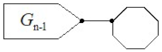
The graph discussed in this article is a connected graph in which no edge is contained in more than one cycle. A cyclooctylene in which no octagon has more than two cut-vertices is called a cyclooctylene chain. Obviously, each cyclooctylene chain contains exactly two octagons with only one cut-vertex. Those octagons are called terminal, all other octagons are internal. The number of octagons in a given cyclooctylene chain is called its length. Additionally, a cyclooctylene chain
with
n octagons can be regarded as an octagonal chain
with
octagons to which a new terminal octagon has been adjoined by an edge, see
Figure 1.
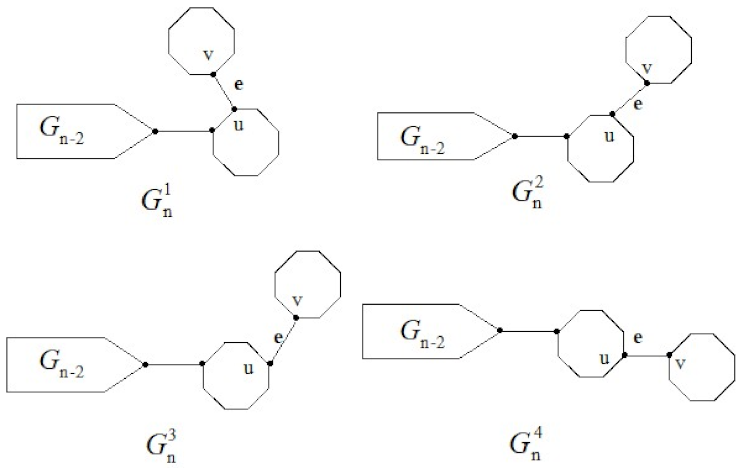
For
, the final octagon can be joined in four manners, these connections can be represented by the following symbols:
, see
Figure 2.
A random cyclooctylene chain
with
n octagons, it is formed by continuing to join the octagons at the end of the last octagon in a cyclooctylene chain. At each step
, there are four different possible ways to connect, as shown below:
where the probabilities
are constants, irrelative to the step parameter
k.
Specially, is the ortho-chain , the meta-chain and the para-chain for and , respectively.
2. The Expected Value of the Hosoya Index of a Random Cyclooctylene Chain
According to the description in the previous section, the octagonal chain
is obtained at random by attaching
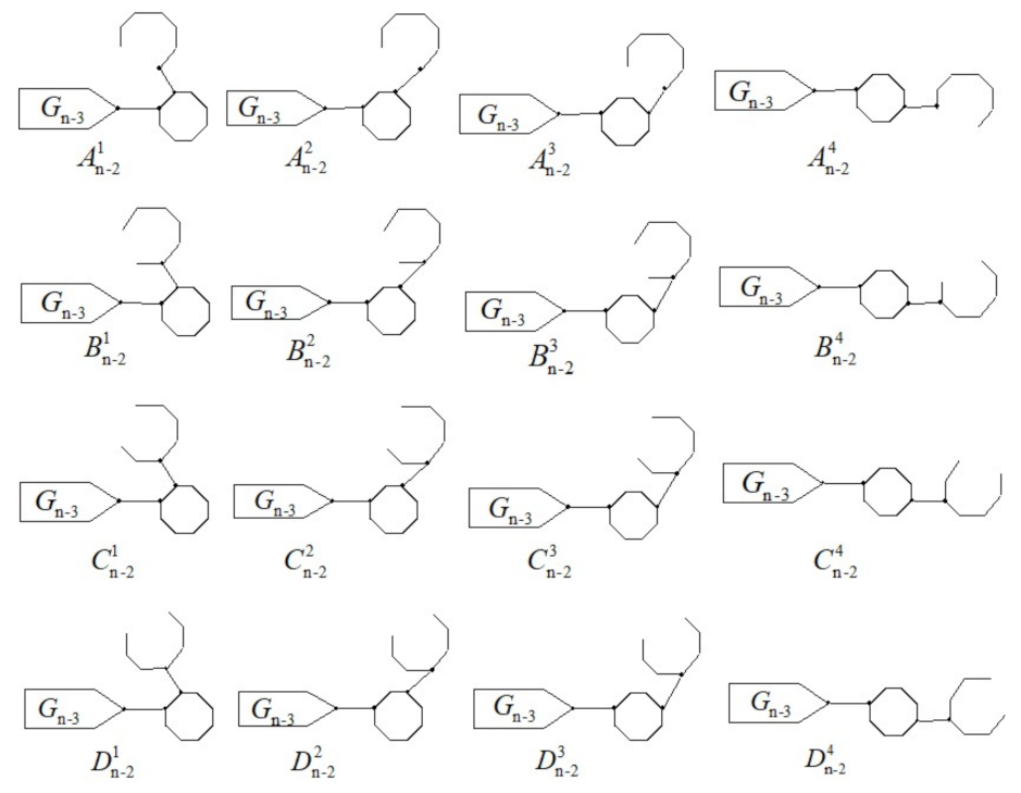
, a new terminal octagon from one of the four possible constructions. This connection method is called a zeroth-order Markov Process. For
, the Hosoya index is a random variable. In the second argument section, we are going to obtain a simple exact formula of its expected value
. There are four types of auxiliary random graphs
and
, where
and
shown in
Figure 3.
- (I)
If
in
Figure 2, then by Equations (1) and (3),
- (i)
If
in
Figure 3, then by Equations (1) and (3),
Similarly, we have:
- (ii)
If , then
- (iii)
If , then
- (iv)
If , then
- (II)
If
in
Figure 2, then by Equations (1) and (3),
- (i)
If
in
Figure 3, then by Equations (1) and (3),
Similarly, we have:
- (ii)
If , then
- (iii)
If , then
- (iv)
If , then
- (III)
If
in
Figure 2, then by Equations (1) and (3),
- (i)
If
in
Figure 3, then by Equations (1) and (3),
Similarly, we have:
- (ii)
If , then
- (iii)
If , then
- (iv)
If , then
- (IV)
If
in
Figure 2, then by Equations (1) and (3),
- (i)
If
in
Figure 3, then by Equations (1) and (3),
Similarly, we have:
- (ii)
If , then
- (iii)
If , then
- (iv)
If , then
Note that , using the formulas in (I) to (IV), we can obtain the expected value .
. Then,
Similarly, we can obtain the expected values
of
,
of
,
of
and
of
,
From Equations (4), (5), (6), (7) and (8), respectively, we have
Substituting these formulas into Equations (4), we have
A recurrence relation for the expected value of the Hosoya index of a random cyclooctylene chain is obtained
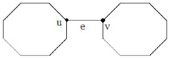
The boundary condition is
,
(According to the
Figure 4).
Using the above recurrence relation and the boundary conditions, we have
Theorem 1. The expected value of the Hosoya index of a random cyclooctylene chain is Let and , , respectively, we can obtain the Hosoya indices of the ortho-chain , the meta-chain and the para-chain from Theorem 1.
3. The Expected Value of the Merrifield–Simmons Index of a Random Cyclooctylene Chain
In this section, we will present a simple exact formula of its expected value .
- (I)
If
in
Figure 2, then by Equations (2) and (3),
- (i)
If
in
Figure 3, then by Equations (2) and (3),
Similarly, we have:
- (ii)
If , then
- (iii)
If , then
- (iv)
If , then
- (II)
If
in
Figure 2, then by Equations (2) and (3),
- (i)
If
in
Figure 3, then by Equations (2) and (3),
Similarly, we have:
- (ii)
If , then
- (iii)
If , then
- (iv)
If , then
- (III)
If
in
Figure 2, then by Equations (1.2) and (1.3),
- (i)
If
in
Figure 3, then by Equations (2) and (3),
Similarly, we have:
- (ii)
If , then
- (iii)
If , then
- (iv)
If , then
- (IV)
If
in
Figure 2, then by Equations (2) and (3),
- (i)
If
in
Figure 3, then by Equations (2) and (3),
Similarly, we have:
- (ii)
If , then
- (iii)
If , then
- (iv)
If , then
Note that , using the formulas in (I) to (IV), we can get the expected value .
. Then,
Similarly, we can obtain the expected values
of
,
of
,
of
and
of
,
From Equations (10), (11), (12), (13) and (14), respectively, we have
Substituting these formulas into Equations (10), we have
A recurrence relation for the expected value of the Merrifield–Simmons index of a random cyclooctylene chain is obtained
.
The boundary condition is
,
(According to the
Figure 4)
Using the above recurrence relation and the boundary conditions, we have
Theorem 2. The expected value of the Merrifield–Simmons index of a random cyclooctylene chain is Let and , , respectively, we can obtain the Merrifieid–Simmons indices of the ortho-chain , the meta-chain and the para-chain from Theorem 2.
4. The Average Value of Hosoya Index and Merrifield–Simmons Index
Let
be the set of all cyclooctylene chains with
n octagons. The average values of the Hosoya index and the Merrifield–Simmons index with respect to
are
In order to obtain the average values , we only need to take in the expected values . From Theorems 1 and 2, we have
Theorem 3. The average value of the Hosoya index and the Merrifield–Simmons index with respect to are Surprisingly, Theorem 3. shows that the average values of the Hosoya index and the Merrifield–Simmons index with respect to are just the expected values of the Hosoya index and the Merrifield–Simmons index of the metachain .
5. Discussion
Previously, many people have analyzed and studied the Hosoya index and Merrifield–Simmons index , for example, similar contents to the ones in this paper have been studied in the random polyethylene chains, that is, studying the two indexes of connectting the hexagonal chemical chain at the end, and obtaining the index expectation of different connection modes at the end according to the relevant known conclusions, on the basis of obtaining the probability of different connection modes of the terminal hexagon, the exponential problem of three different chains is further solved.
According to the relevant contents of the hexagon introduced before, in this article, we further push down and obtain the end connected octagon. Firstly, a series of exact formulas to push the Hosoya index and the Merrifield–Simmons index are presented, and the two indexes of the simple graph used in the later research process are calculated. Then, the corresponding chemical diagrams in the calculation process are depicted by drawing software through different connection methods. Finally, different formulas and corresponding graphs are combined to obtain the expected values of the two indexes of the random cyclooctylene chain with n octagons; it is inferred that four different probabilities represent different connection modes of terminal octagons, which means that there are accurate values of the Hosoya index and the Merrifield–Simmons index of four chemical chains, meanwhile, we also obtain the average value with respect to the set of all the random cyclooctylene chains.
6. Concluding Remarks
There are still some limitations and problems for further study in this paper. Firstly, for the graphs studied by Hosoya index and Merrifield–Simmons index, they are all finite simple and directional graphs with special restriction conditions. Therefore, there are many problems related to different graphs that have not been solved for later discussion and study. Secondly, the exact formula given in the process of research expectation is only one research method. There are many different ways to solve the two indices, and different ways have different advantages and disadvantages. Finally, there are still many questions about the different indices of different chemical chains that require further study and characterization. This paper only presents the Hosoya index and Merrifield–Simmons index of random cyclooctylene chains, cyclooctylene and their derivatives have attracted a lot of attention, and their composition and structure are also being studied in the direction of graph theory.
Author Contributions
Conceptualization, Y.S. and X.G.; methodology, Y.S.; software, Y.S.; validation, Y.S., X.G.; formal analysis, Y.S.; investigation, Y.S.; resources, Y.S.; data curation, Y.S.; writing—original draft preparation, Y.S.; writing—review and editing, Y.S.; visualization, Y.S.; supervision, Y.S.; project administration, Y.S.; funding acquisition, X.G. All authors have read and agreed to the published version of the manuscript.
Funding
The research is partially supported by National Science Foundation of China (Grant No. 12171190) and Natural Science Foundation of Anhui Province (Grant No. 2008085MA01).
Institutional Review Board Statement
Not applicable.
Informed Consent Statement
Not applicable.
Data Availability Statement
Not applicable.
Acknowledgments
The authors are very grateful to the helpful comments and suggestions. The research is partially supported by National Science Foundation of China (Grant No. 12171190) and Natural Science Foundation of Anhui Province (Grant No. 2008085MA01).
Conflicts of Interest
The authors declare no conflict of interest.
References
- Bureš, M.; Pekárek, V.; Ocelka, T. Thermochemical properties and relative stability of polychlorinated. Environ. Toxicol. Pharm. 2008, 25, 2610–2617. [Google Scholar] [CrossRef] [PubMed]
- Chen, X.; Zhao, B.; Zhao, P. Six-membered ring spiro chains with extremal Merrifield-Simmons index and Hosoys index. MATCH Commun. Math. Comput. Chem. 2009, 62, 657–665. [Google Scholar]
- Gao, Y.D.; Hosoya, H. Topological index and thermodynamic properties. IV. Size dependency of the structure activity correlation of alkanes. Bull. Chem. Soc. Jpn. 1988, 61, 3093–3102. [Google Scholar] [CrossRef]
- Gutman, I. A regularity for the boiling points of alkanes and its mathematical modeling. Z. Phys Chem. 1986, 267, 1152–1158. [Google Scholar] [CrossRef]
- Graja, A. Low-Dimensional Organic Conductors; World Scientific: Singapore, 1992. [Google Scholar]
- Hosoya, H.; Gotoh, M.; Murakami, M.; Ikeda, S. Topological index and thermodynamic properties. 5. How can we explain the topological dependence of thermodynamic properties of alkanes with thetopology of graphs? J. Chem. Inf. Comput. Sci. 1999, 39, 192–196. [Google Scholar] [CrossRef]
- Hosoya, H.; Hosoi, K. Topological index as applied to π-electron systems. III. Mathematical relations among various bond orders. J. Chem. Phys. 1976, 64, 1065–1073. [Google Scholar] [CrossRef]
- Hosoya, H.; Murakami, M. Topological index as applied to π-electronic systems. II. Topological bond order. J. Chem. Soc. Jpn. 1975, 48, 3512–3517. [Google Scholar] [CrossRef]
- Liu, Y.; Zhuang, W.; Liang, Z. Largest Hosoya index and smallest Merrifield-Simmons index in tricyclicgraphs. MATCH Commun. Math. Comput. Chem. 2015, 73, 195–224. [Google Scholar]
- Narumi, H.; Hosoya, H. Topological index and thermodynamic properties. II. Analysis of the topological factors on the absolute entropy of acyclic saturated hydrocarbons. Bull. Chem. Soc. Jpn. 1980, 53, 1228–1237. [Google Scholar] [CrossRef]
- Narumi, H.; Hosoya, H. Topological index and thermodynamic properties. III. Classification of various topological aspects of properties of acyclic saturated hydro carbons. Bull. Chem. Soc. Jpn. 1985, 58, 1778–1786. [Google Scholar] [CrossRef]
- Simmons, H.E.; Merrifield, R.E. Mathematical description of molecular structure; molecular topology. Proc. Natl. Acad. Sci. USA 1977, 742, 2616–2619. [Google Scholar] [CrossRef] [PubMed]
- Gutman, I.; Furtula, B.; Vidović, D.; Hosoya, H. A concealed property of the topological index Z. Bull. Chem. Soc. Jpn. 2004, 77, 491–496. [Google Scholar] [CrossRef]
- Gutman, I.; Polansky, O.E. Mathematical Concepts in Organic Chemistry; Springer: Berlin, Germany, 1986. [Google Scholar]
- Gutman, I.; Yamaguchi, T.; Hosoya, H. Topological index as applied to π-electronic systems. IV. On the topological factors causing non-uniform π-electron charge distribution in non-alternant hydrocarbons. Bull. Chem. Soc. Jpn. 1976, 49, 1811–1816. [Google Scholar] [CrossRef]
- Huang, G.; Kuang, M.; Deng, H. The expect values of Hosoya index and Merrifield-Simmons index in a random polyphenylene. J. Comb. Optim. 2016, 32, 550–562. [Google Scholar] [CrossRef]
- Hosoya, H. Graphical enumeration of the coefficients of the secular polynomials of the Hückel molecular orbitals. Theor. Chim. Acta 1975, 25, 215–222. [Google Scholar] [CrossRef]
- Hosoya, H. Chemical meaning of octane number analyzed by topological indices. Croat Chem. Acta 2002, 75, 433–445. [Google Scholar]
- Hosoya, H.; Hosoi, K.; Gutman, I. A topological index for the total π-electron energy. Proof of a generalized Hückel rule for an arbitrary network. Theor. Chim. Acta 1975, 38, 37–47. [Google Scholar] [CrossRef]
- Merrifield, R.E.; Simmons, H.E. Topological Methods in Chemistry; Wiley: New York, NY, USA, 1989. [Google Scholar]
- Zhu, Z.; Yuan, C.; Andriantiana, E.O.D.; Wagner, S. Graphs with maximal Hosoya index and minimal Merrifield-Simmons index. Discret. Math. 2014, 329, 77–87. [Google Scholar] [CrossRef]
- Zhao, P.; Zhao, B.; Chen, X.; Bai, Y. Two classes of chains with maximal and minmal total π-electron energy. MATCH Commun. Math. Comput. Chem. 2009, 62, 525–536. [Google Scholar]
- Merrifield, R.E.; Simmons, H.E. Enumeration of structure-sensitive graphical subsets: Theory. Proc. Natl. Acad. Sci. USA 1981, 78, 692–695. [Google Scholar] [CrossRef]
- Merrifield, R.E.; Simmons, H.E. Enumeration of structure-sensitive graphical subsets: Calculations. Proc. Natl. Acad. Sci. USA 1981, 78, 1329–1332. [Google Scholar] [CrossRef] [PubMed]
- Merrifield, R.E.; Simmons, H.E. Topology of bonding in π-electron systems. Proc. Natl. Acad. Sci. USA 1985, 82, 1–3. [Google Scholar] [CrossRef] [PubMed]
- Tepavcevie, S.; Wroble, A.T.; Bissen, M.; Wallace, D.J.; Choi, Y.; Hanley, L. Photoemission studies of polythiophene and polyphenyl films produced via surface polymerization by ion-assisted deposition. J. Phys. Chem. B 2005, 109, 7134–7140. [Google Scholar] [CrossRef] [PubMed]
- Yang, W.; Zhang, F. Wiener index in random polyphenyl chains. MATCH Commun. Math. Comput. Chem. 2012, 68, 371–376. [Google Scholar]
- Andriatiana, E.O.D. Energy, Hosoys index and Merrifield-Simmons index of trees with prescribed degree sequence. Discret. Appl. Math. 2013, 161, 724–741. [Google Scholar] [CrossRef]
- Hosoya, H. Topological index. A newly proposed quantity characterizing the topological nature of structural isomers of saturated hydrocarbons. Bull. Chem. Soc. Jpn. 1971, 44, 2332–2339. [Google Scholar] [CrossRef]
- Luthe, G.; Jacobus, J.A.; Robertson, L.W. Receptor interactions by polybrominated diphenyl ethers versus polychlorinated biphenyls:a theoretical structure-activity assessment. Environ. Toxicol. Pharm. 2008, 25, 202–210. [Google Scholar] [CrossRef] [PubMed]
- Deng, H. Wiener indices of spiro and polyphenyl hexagonal chains. Math. Comput. Model. 2012, 55, 634–644. [Google Scholar] [CrossRef]
- Deng, H.; Tang, Z. Kirchhoff indices of spiro and polyphenyl hexagonal chains. Util. Math. 2014, 95, 113–128. [Google Scholar]
- Došlić, T.; Litz, M. Matchings and independent sets in polyphenylene chains. MATCH Commun. Math. Comput. Chem. 2012, 67, 313–330. [Google Scholar]
- Flower, D.R. On the properties of bit string-based measures of chemical similarity. Chem. Inf. Comput. Sci. 1998, 38, 379–386. [Google Scholar] [CrossRef]
- Merrifield, R.E.; Simmons, H.E. The structure of molecular topological spaces. Theor. Chim. Acta 1980, 55, 55–757. [Google Scholar] [CrossRef]
- Bai, Y.; Zhao, B.; Zhao, P. Extremal Merrifield-Simmons index and Uosoya index of polyphenyl chains. MATCH Commun. Math. Comput. Chem. 2009, 62, 649–656. [Google Scholar]
- Došlić, T.M.; ȧloy, F. Chain hexagonal cacti: Matchings and independent set. Discret. Math. 2010, 310, 1676–1690. [Google Scholar] [CrossRef]
- Hosoya, H.; Kawasaki, K.; Mizutani, K. Topological index and thermodynamic properties. I. Empirical rules on the boiling point of saturated hydrocarbons. Bull. Chem. Soc. Jpn. 1972, 45, 3415–3421. [Google Scholar] [CrossRef]
- Narumi, H. Statistico-mechanical aspect of the Hosoya index. Int. El J. Mol. Des. 2003, 2, 375–382. [Google Scholar]
- Wagner, S.; Gutman, I. Maxima and minima of the Hosoya index and the Merrifield-Simmons index. Acta Appl. Math. 2010, 112, 323–346. [Google Scholar] [CrossRef]
- Gutman, I.; Vidović, D.; Hosoya, H. The relation between the eigenvalue sum and the topological index Z revisited. Bull. Chem. Soc. Jpn. 2002, 75, 1723–1727. [Google Scholar] [CrossRef]
| Publisher’s Note: MDPI stays neutral with regard to jurisdictional claims in published maps and institutional affiliations. |
© 2022 by the authors. Licensee MDPI, Basel, Switzerland. This article is an open access article distributed under the terms and conditions of the Creative Commons Attribution (CC BY) license (https://creativecommons.org/licenses/by/4.0/).


