Toroidal Spectral Drawing

Abstract

We give a deterministic drawing algorithm to draw a graph onto a torus, which is based on the usual spectral drawing algorithm. For most of the well-known toroidal vertex-transitive graphs, the result drawings give an embedding of the graphs onto the torus.

1. Introduction

Graph drawing is a representation of graphs on Euclidean space such that vertices of the graph are points in Euclidean space and edges are lines or curves between vertices. According to the way of getting the coordinates of vertices, graph drawing algorithms can be divided into two categories: dynamic drawings and deterministic drawings. For dynamic drawings, the coordinates of vertices are usually given by the process of optimizing some potential energy function. For deterministic drawings, the coordinates of the vertices are given by an explicit formula directly.

The spectral drawing algorithm [1,2] is one of most well-known deterministic drawings based on the spectra of graphs. It is also the optimizing drawing respect to the certain potential energy function. Roughly speaking, the spectral drawing is the shortest length drawing among all orthogonal projections drawing. (See Section 1 for details).

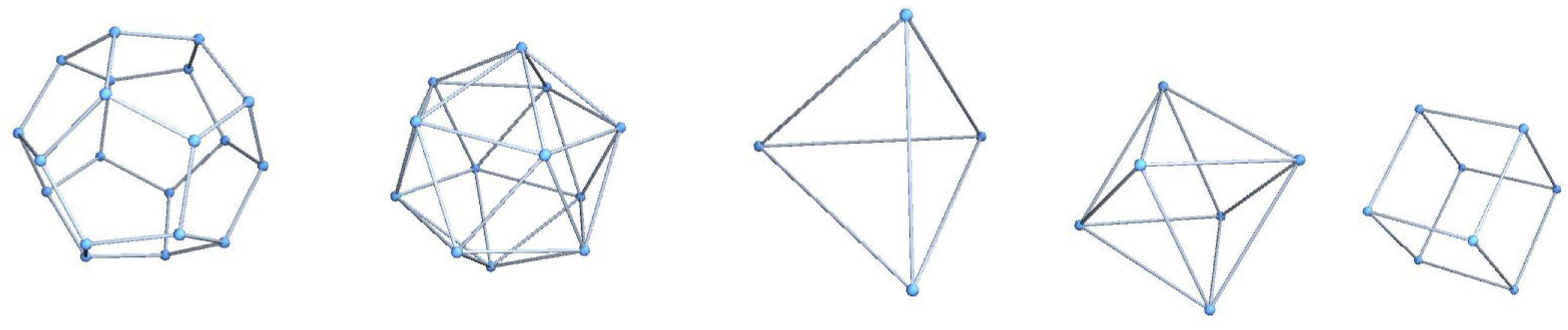
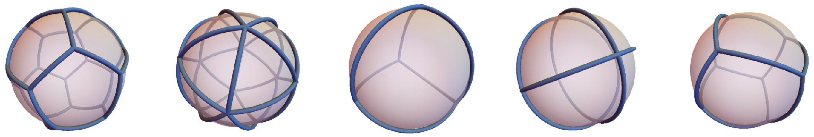
In general, the spectral drawing can draw the highly symmetric planar graph well. For example, Figure 1 shows spectral drawings of the underlying graph of the skeletons of the Platonic solids.

In these examples, the spectral drawing naturally induces an embedding of the graph into the unit sphere in three-dimensional Euclidean space as shown in Figure 2.

However, the spectral drawing does not work well for highly symmetric non-planar graphs. For a non-planer graph, it can be embedded on a closed surface of some genus. When it can be embedded on a surface of genus one, namely a torus, it is called a toroidal graph. For example, the complete graphs $K_5$, $K_6$, and $K_7$ are toroidal graphs. In addition, the Heawood graph and the Peterson graph are also toroidal graphs. Furthermore, there are several infinite families of toroidal Cayley graphs [3]. For those well-known toroidal graphs, their embedding onto a torus can be found in many literature, e.g., [4]. However, there is no systemic way to obtain these embeddings.

There are several studies of drawing graphs on a torus [5,6,7]. However, these approaches do not give explicit drawings directly and they also require the extra structure of graphs, namely the choice of the set of “faces” (or so-called rotation systems).

The main contribution of the paper is to give a deterministic drawing algorithm for highly symmetric toroidal graphs without using any extra structure. The main idea is that for a highly symmetric toroidal graph, we expect that it admits a “shortest-length” drawing on a torus, which can be canonically induced from the usual spectral drawing. We will use vertex-transitive toroidal graphs as our examples, including $K_5$, $K_6$, $K_7$, $K_{3,3}$, the Heawood graph, some generalized Petersen graphs, and toroidal fullerence graph. For these toroidal graphs, our algorithm gives each of them an embedding on a torus except for generalized Petersen graphs.

2. Spectral Drawing Revisited

In this section, we recall the spectral drawing algorithm and explain why it works well for highly symmetric planar graphs like the skeletons of the platonic solids. Let $\mathcal{X}=(\mathcal{V},\mathcal{E})$ be a connected undirected graph with n vertices.

2.1. Symmetric Drawings

A straight-line drawing $\rho$ of $\mathcal{X}$ onto the inner product space $(W,\langle ·,·\rangle )$ is a map from $\mathcal{V}$ to W such that

• the vertex v is represented by the point $\rho \left(v\right)$.
• the edge $(v,v^{\prime })$ is represented by the straight line segment between $\rho \left(v\right)$ and $\rho \left(v^{\prime }\right)$.

We say $\rho$ is a symmetric drawing if for any graph automorphism $\sigma$ of $\mathcal{X}$, there exists a linear isometry $\tilde{\sigma }$ of W such that for all $v\in \mathcal{V}$,

$$\rho \circ \sigma \left(v\right)=\tilde{\sigma }\circ \rho \left(v\right).$$

In other words, a symmetric drawing preserves all symmetries of the graph.

2.2. Regular Drawings

Let $\mathbb{R}\left[\mathcal{V}\right]$ be a real inner product space with an orthonormal basis $\left\{{\overrightarrow{e}}_v\right|v\in \mathcal{V}\}$. The regular drawing ${\rho }_{{}_{reg}}$ of $\mathcal{X}$ is a straight-line drawing onto $\mathbb{R}\left[\mathcal{V}\right]$ which maps v to ${\overrightarrow{e}}_v$. For an automorphism $\sigma$ of $\mathcal{X}$, let ${\rho }_{\sigma }$ be a linear transformation on $\mathbb{R}\left[\mathcal{V}\right]$ characterized by

$${\rho }_{\sigma }\left({\overrightarrow{e}}_v\right)={\overrightarrow{e}}_{\sigma \left(v\right)}\mathrm{for} \mathrm{all} v\in \mathcal{V}.$$

Since ${\rho }_{\sigma }$ permutes the orthonormal basis, it is an isometry. In addition, we have

$${\rho }_{{}_{reg}}\circ \sigma \left(v\right)=e_{\sigma \left(v\right)}={\rho }_{\sigma }\circ {\rho }_{{}_{reg}}\left(v\right).$$

We conclude that ${\rho }_{{}_{reg}}$ is a symmetric drawing.

2.3. Spectral Drawing Algorithm

The Laplacian operator L of $\mathcal{X}$ is a linear transformation on $\mathbb{R}\left[\mathcal{V}\right]$ characterized by

$$L\left({\overrightarrow{e}}_v\right)=\sum _{(v,v^{\prime })\in \mathcal{E}}{\overrightarrow{e}}_v-{\overrightarrow{e}}_{v^{\prime }}$$

The Laplacian operator is positive semi-definite with eigenvalues

$$0={\lambda }_1<{\lambda }_2\le {\lambda }_3\le \cdots \le {\lambda }_n.$$

Let $\left\{{\overrightarrow{u}}_1,\cdots ,{\overrightarrow{u}}_n\right\}$ be the corresponding orthonormal eigenbasis such that $L\left({\overrightarrow{u}}_i\right)={\lambda }_i{\overrightarrow{u}}_i$ for all i. Let $U_k$ be the k-dimensional subspace of $\mathbb{R}\left[\mathcal{V}\right]$ spanned by $\{{\overrightarrow{u}}_2,\cdots ,{\overrightarrow{u}}_{k+1}\}$. The k-dimensional spectral drawing ${\mathrm{Spd}}_k$ is a straight-line drawing given by

$${\mathrm{Spd}}_k\left(v\right):={\mathrm{proj}}_{U_k}\left({\overrightarrow{e}}_v\right).$$

Here ${\mathrm{proj}}_{U_k}\left(\overrightarrow{x}\right)$ is the orthogonal projection onto $U_k$.

2.4. Potential Energy Function of Spectral Drawing Algorithm

Given a k-dimensional subspace W of $\mathbb{R}\left[\mathcal{V}\right]$, define the energy function of W as

$$E\left(W\right):=\sum _{(v,w)\in \mathcal{E}}{\parallel {\mathrm{proj}}_W\left({\overrightarrow{e}}_v\right)-{\mathrm{proj}}_W\left({\overrightarrow{e}}_w\right)\parallel }^2.$$

Suppose $\{{\overrightarrow{\alpha }}_1,\cdots ,{\overrightarrow{\alpha }}_k\}$ is an orthonormal basis of W. Then we have

$$\parallel {\mathrm{proj}}_W\left({\overrightarrow{e}}_v\right)-{\mathrm{proj}}_W\left({\overrightarrow{e}}_w\right){\parallel }^2=\sum _{i=1}^k{\left(\langle {\overrightarrow{e}}_v,{\overrightarrow{\alpha }}_i\rangle -\langle {\overrightarrow{e}}_w,{\overrightarrow{\alpha }}_i\rangle \right)}^2.$$

Hence, one can rewrite the energy function as

$$E\left(W\right)=\sum _{i=1}^k\sum _{(v,w)\in \mathcal{E}}{\left(\langle {\overrightarrow{e}}_v,{\overrightarrow{\alpha }}_i\rangle -\langle {\overrightarrow{e}}_w,{\overrightarrow{\alpha }}_i\rangle \right)}^2=\sum _{i=1}^k{\langle {\overrightarrow{\alpha }}_i,L\left({\overrightarrow{\alpha }}_i\right)\rangle }^2.$$

Therefore, subject to the condition $W\perp {(1,\cdots ,1)}^t$, $E\left(W\right)$ is minimal if W is spanned by eigenvectors of L corresponding to ${\lambda }_2,\cdots ,{\lambda }_{k+1}$. In other words, the k-dimensional spectral drawing has the minimal energy among all drawings arising from the projections onto k-dimensional subspaces.

2.5. Spectral Drawings and Symmetric Drawings

The following theorem shows when the spectral drawing is a symmetric drawing.

Theorem 1.

When $U_k$ is a direct sum of eigenspaces $E\left(\lambda \right)$ of L, $U_k$ is ${\rho }_{\sigma }$ invariant for any automorphism σ of $\mathcal{X}$ and ${\mathrm{Spd}}_k$ is a symmetric drawing.

Proof. 

Let $\sigma$ be an automorphism of $\mathcal{X}$. First, let us show that the isometry ${\rho }_{\sigma }$ and L commute. For any $v\in \mathcal{V}$,

$$\begin{array}{cc}\hfill {\rho }_{\sigma }\left(L\left({\overrightarrow{e}}_v\right)\right)& ={\rho }_{\sigma }\left(\sum _{(v,v^{\prime })\in \mathcal{E}}{\overrightarrow{e}}_v-{\overrightarrow{e}}_{v^{\prime }}\right)\hfill \\ \hfill & =\sum _{(v,v^{\prime })\in \mathcal{E}}{\overrightarrow{e}}_{\sigma \left(v\right)}-{\overrightarrow{e}}_{\sigma \left(v^{\prime }\right)}=\sum _{(\sigma \left(v\right),\sigma \left(v^{\prime }\right))\in \mathcal{E}}{\overrightarrow{e}}_{\sigma \left(v\right)}-{\overrightarrow{e}}_{\sigma \left(v^{\prime }\right)}\hfill \\ \hfill & =\sum _{(\sigma \left(v\right),v^{\prime \prime })\in \mathcal{E}}{\overrightarrow{e}}_{\sigma \left(v\right)}-{\overrightarrow{e}}_{v^{″}}=L\left({\rho }_{\sigma }\left({\overrightarrow{e}}_v\right)\right).\hfill \end{array}$$

Next, we show that $U_k$ is ${\rho }_{\sigma }$-invariant. Suppose $\overrightarrow{u}$ is a $\lambda$-eigenvector of L in $U_k$. Then

$$L\left({\rho }_{\sigma }\left(\overrightarrow{u}\right)\right)={\rho }_{\sigma }\left(L\left(\overrightarrow{u}\right)\right)={\rho }_{\sigma }\left(\lambda \overrightarrow{u}\right)=\lambda {\rho }_{\sigma }\left(\overrightarrow{u}\right).$$

Therefore, $\overrightarrow{u}$ is also a $\lambda$-eigenvector and it is contained in $U_k$. We conclude that $U_k$ is ${\rho }_{\sigma }$-invariant, or equivalently ${\mathrm{proj}}_{U_k}$ and ${\rho }_{\sigma }$ commute. Finally, set $\tilde{\sigma }=\sigma {|}_{U_k}$. Then for all $v\in \mathcal{V}$,

$${\mathrm{Spd}}_k\left(\sigma \left(v\right)\right)={\mathrm{proj}}_{U_k}\left({\overrightarrow{e}}_{\sigma \left(v\right)}\right)={\mathrm{proj}}_{U_k}\left({\rho }_{\sigma }\left({\overrightarrow{e}}_v\right)\right)={\rho }_{\sigma }\left({\mathrm{proj}}_{U_k}\left({\overrightarrow{e}}_v\right)\right)=\tilde{\sigma }\left({\mathrm{Spd}}_k\left(v\right)\right).$$

Therefore, ${\mathrm{Spd}}_k$ is a symmetric drawing. □

Example 1.

When $\mathcal{X}$ is the underlying graph of the skeleton of a platonic solid, we always have ${\lambda }_2={\lambda }_3={\lambda }_4<{\lambda }_5$. (This can be verified by direct computation.) Therefore, the 3-dimensional spectral drawing of $\mathcal{X}$ is a symmetric drawing.

2.6. Partially Symmetric Drawing

Note that the subspace $U_k$ is not unique when $U_k$ is not a direct sum of eigenspace of L. For example, when ${\lambda }_2={\lambda }_3={\lambda }_4={\lambda }_5$, then $U_3$ can be any three dimensional subspace of $E\left({\lambda }_2\right)$. In this case, we need an extra structure to obtain a good choice of $U_3$.

To do so, fix an automorphism $\sigma$ of $\mathcal{X}$ and let ${\rho }_{\sigma }$ be the isometry on $\mathbb{R}\left[\mathcal{V}\right]$ given in Section 2.2. Then the restriction of ${\rho }_{\sigma }$ on $E\left(\lambda \right)$ is still an isometry. Recall the following theorem of linear isometries.

Theorem 2

([8] Theorem 6.46). Let T be a linear isometry on a nonzero-real finite dimensional real inner product space W. Then there exists a collection of pairwise orthogonal T-invariant subspaces $\{W_1,\cdots ,W_m\}$ of V such that

(a) 

$dim\left(W_i\right)=1$ or 2 for all i.

(b) 

$W=W_1\oplus \cdots \oplus W_m$.

(c) 

When $dim\left(W_i\right)=1$, $T{|}_{W_i}=1$ or $-1$.

(d) 

When $dim\left(W_i\right)=2$, $T{|}_{W_i}$ is a rotation with non-real eigenvalues. In this case, $W_i$ is is called a rotational plane of T.

Applying the above theorem to all eigenspaces of L, we have the following result.

Theorem 3.

Given an isometry σ of $\mathcal{X}$, there exists a decomposition $\mathbb{R}\left[\mathcal{V}\right]=\oplus W_i$ such that for all i,

1. 

$W_i$ is contained in some eigenspace of L.

2. 

$W_i$ is ${\rho }_{\sigma }$-invariant.

3. 

$W_i$ is either of one dimension or it is a rotational plane of ${\rho }_{\sigma }$.

Note that for a rotational plane $W_i$ in the above theorem, the projection from $\mathbb{R}\left[\mathcal{V}\right]$ to $W_i$ induces a planar drawing of the graph $\mathcal{X}$ which preserves the symmetry $\sigma$. In this case, we say the resulted drawing is partially symmetric.

3. Toroidal Graph Drawing

In this section, we propose a deterministic algorithm to draw highly symmetric toroidal graphs on a torus. We shall use ${(\mathbb{R}/2\pi \mathbb{Z})}^2$ as the model of the torus.

3.1. The Drawing Algorithm

Let $\mathcal{X}=(\mathcal{V},\mathcal{E})$ be an undirected connected graph with the set of vertices $\mathcal{V}=\{v_1,\cdots ,v_n\}$. Fix an automorphism $\sigma$ of $\mathcal{X}$, which can be chosen to be of maximal order or any specific symmetry that we would like to preserve. Suppose that ${\rho }_{\sigma }$ contains at least two rotational planes. The following is our proposed algorithm.

1.

Find two mutually orthogonal rotational plane $W_1$ and $W_2$ of ${\rho }_{\sigma }$ such that each $W_i$ is contained in some eigenspace $E\left({\lambda }_i\right)$ of L with the smallest possible ${\lambda }_i$.

2.

Find an orthonormal basis $\{{\overrightarrow{u}}_1,{\overrightarrow{u}}_2\}$ of $W_1$ and an orthonormal basis $\{{\overrightarrow{u}}_3,{\overrightarrow{u}}_4\}$ of $W_2$.

3.

Write ${\overrightarrow{u}}_i={(u_{i1},\cdots ,u_{in})}^T$. Define a map $f:\mathcal{V}\mapsto {(\mathbb{R}/2\pi \mathbb{Z})}^2$ given by $f\left(v_i\right)=({\theta }_i,{\psi }_i)$ which satisfies the following condition.

$$(cos{\theta }_i,sin{\theta }_i,cos{\psi }_i,sin{\psi }_i)=\left(\frac{u_{1i}}{\sqrt{{u_{1i}}^2+{u_{2i}}^2}},\frac{u_{2i}}{\sqrt{{u_{1i}}^2+{u_{2i}}^2}},\frac{u_{3i}}{\sqrt{{u_{3i}}^2+{u_{4i}}^2}},\frac{u_{4i}}{\sqrt{{u_{3i}}^2+{u_{4i}}^2}}\right).$$

Remark 1.

When $\sqrt{{u_{1i}}^2+{u_{2i}}^2}$ or $\sqrt{{u_{3i}}^2+{u_{4i}}^2}$ equals to zero, set ${\theta }_i$ or ${\psi }_i$ to be zero respectively.

4.

For each edge $(v_i,v_j)$, draw a shortest straight line segment between $({\theta }_i,{\psi }_i)$ and $({\theta }_j,{\psi }_j)$ in the space $\mathbb{R}/{\left(2\pi \mathbb{Z}\right)}^2$. (If the shortest straight line segments are not unique, just choose one of them.) Then we obtain a drawing of $\mathcal{X}$ on the torus ${(\mathbb{R}/2\pi \mathbb{Z})}^2$. In addition, combing with the standard parametric equation of the torus in ${\mathbb{R}}^3$, one can also obtain a drawing on ${\mathbb{R}}^3$.

3.2. Examples

In the following examples, we not only draw the graph on ${(\mathbb{R}/2\pi \mathbb{Z})}^2$ but also draw the graph on the torus in ${\mathbb{R}}^3$ using the parametrization

$$f(\theta ,\psi )=\left(\right(R+rcos\theta )cos\psi ,(R+rcos\theta )sin\psi ,rsin\psi )$$

with $(R,r)=(2.5,1)$.

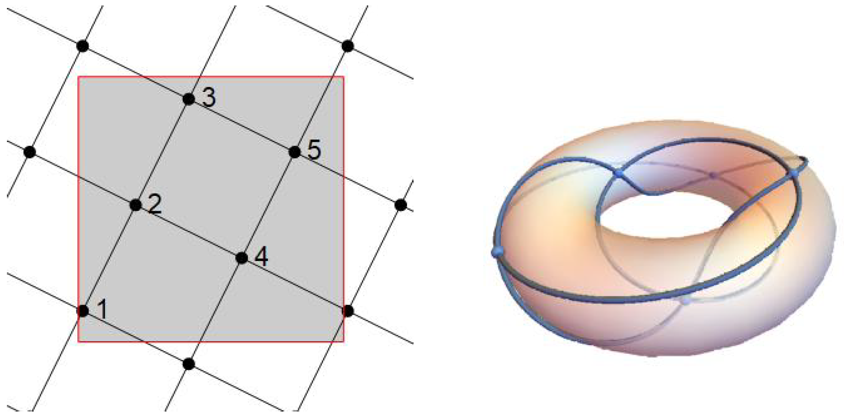
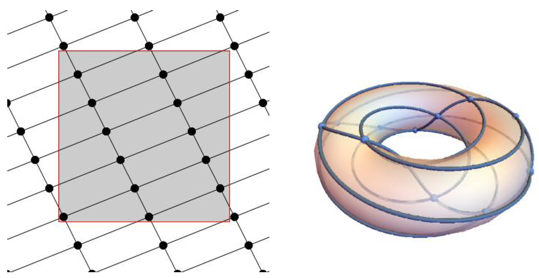
Example 2.

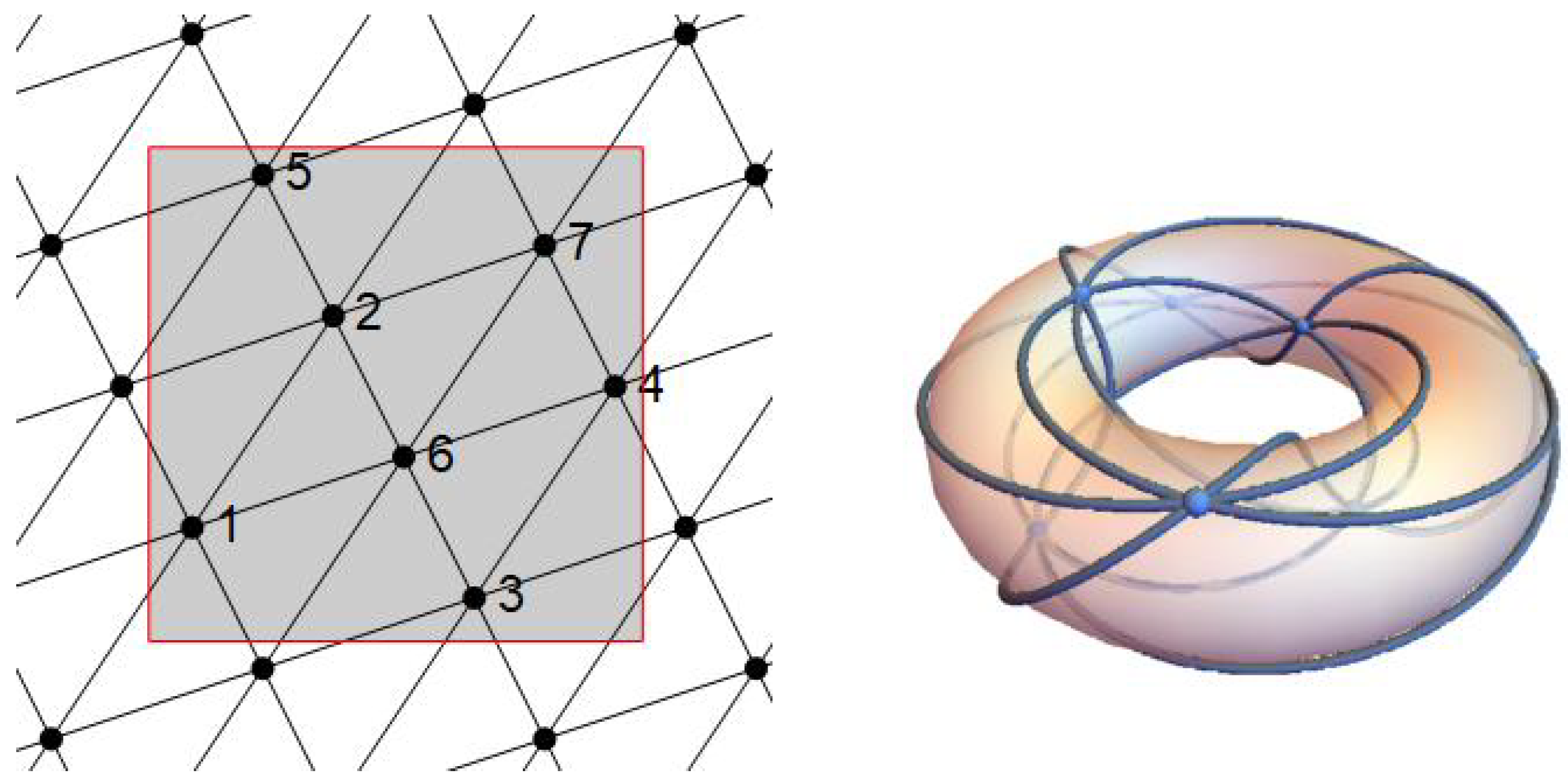
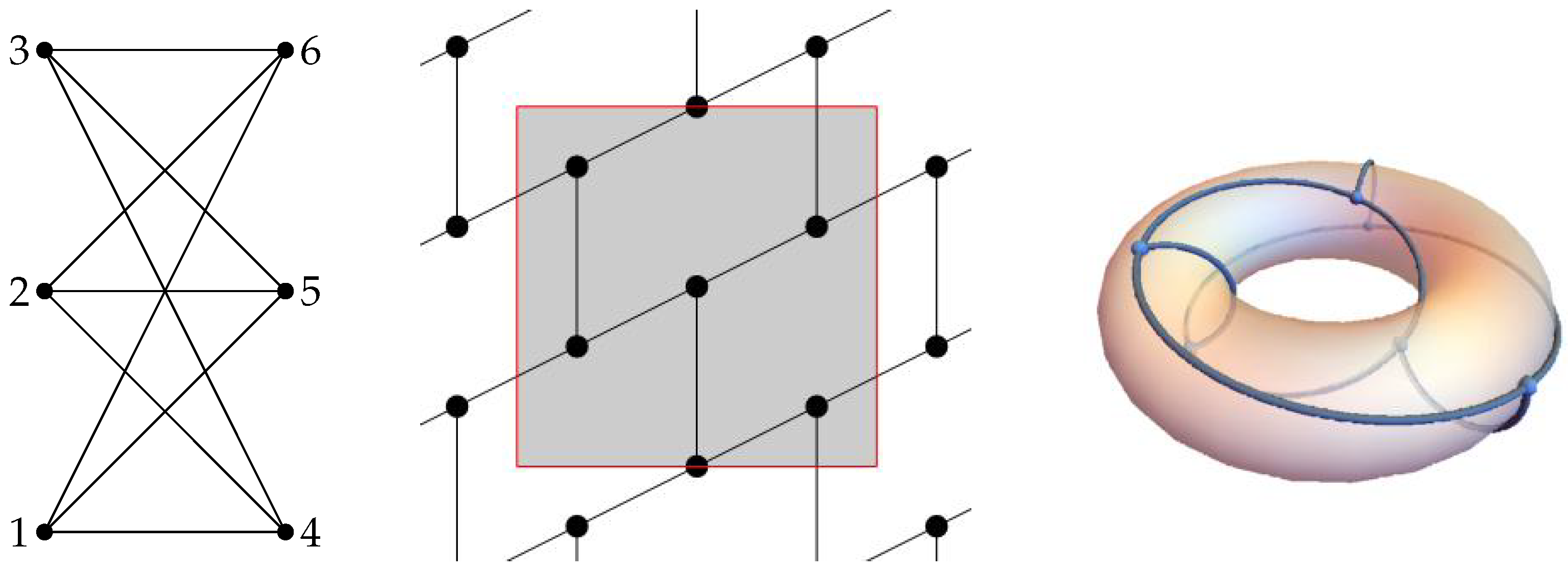
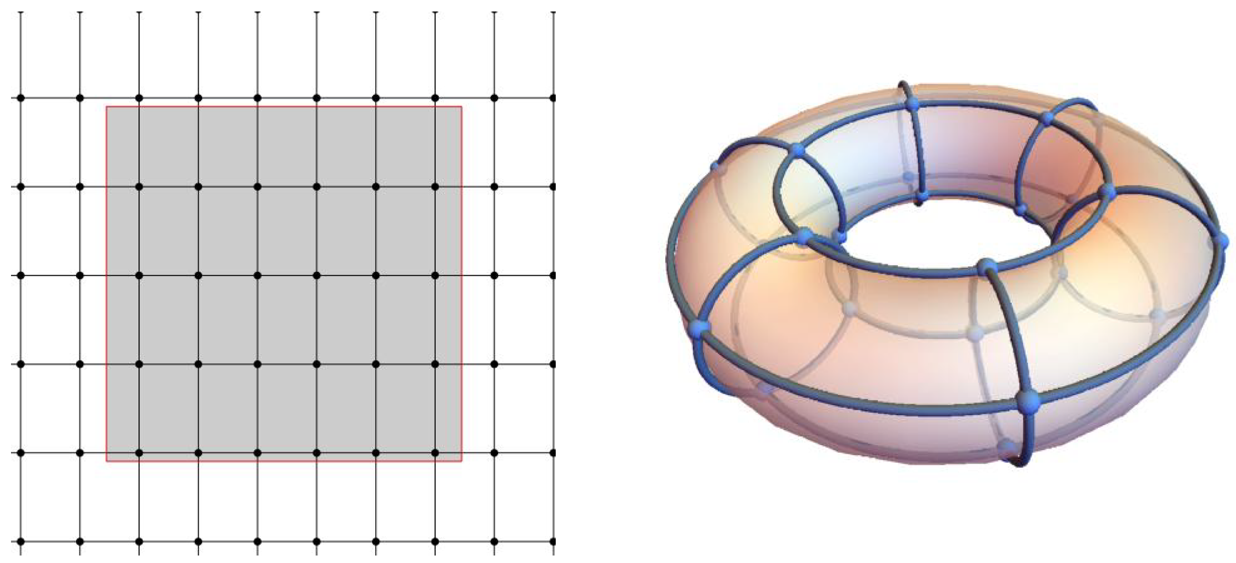
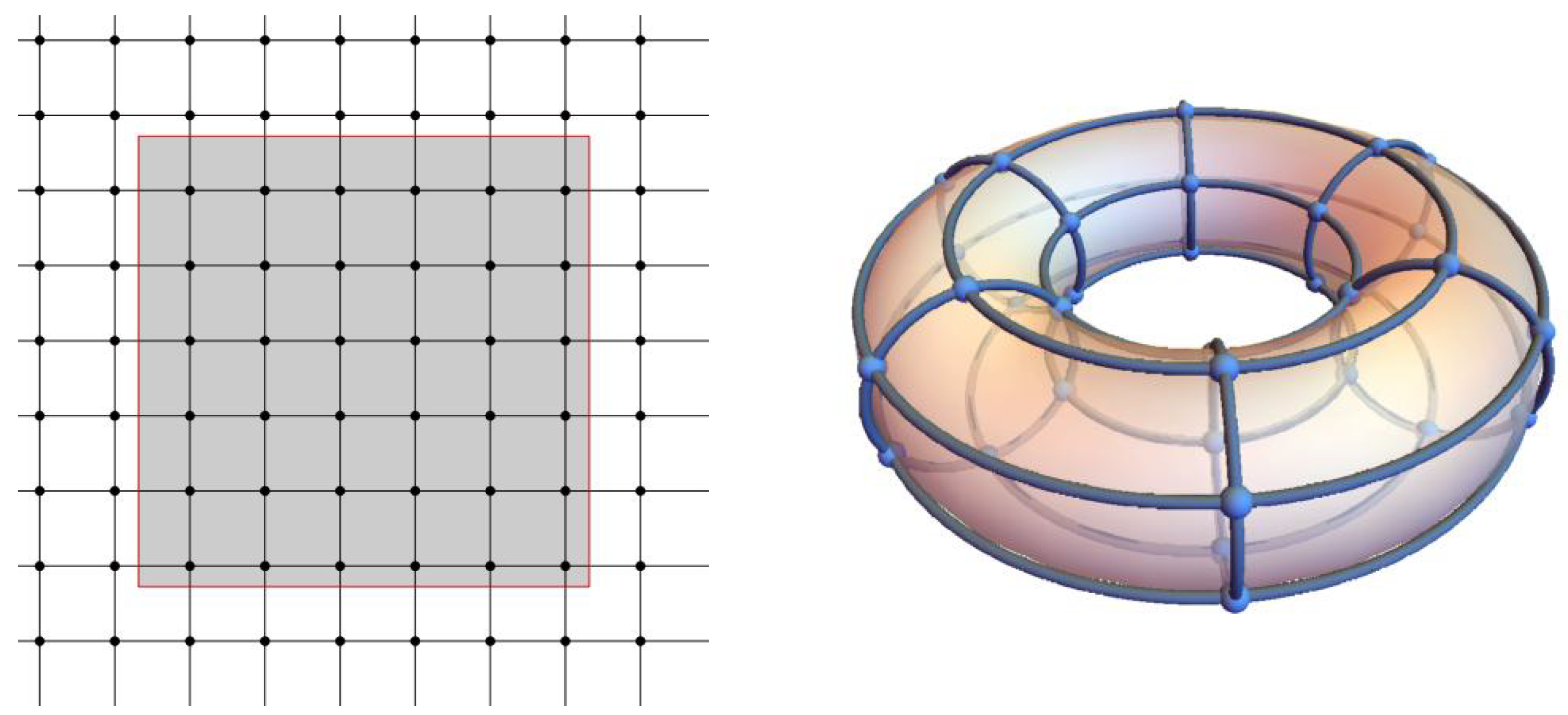
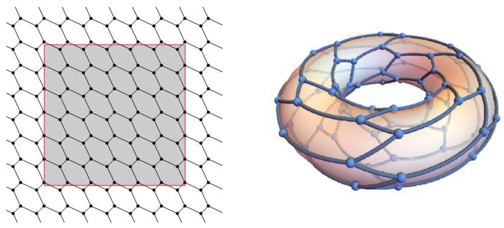
For the graph $K_n$ with n = 5, 6, or 7, the second smallest eigenvalue ${\lambda }_2$ of L equals n, which is of dimension $n-1$. Label the vertices by 1 to n and let $\sigma =(123\cdots n)$ be an automorphism of $K_n$ which is of order n. Choose $W_1$ and $W_2$ to be any two orthogonal rotational planes of ${\rho }_{\sigma }$ in $E\left({\lambda }_2\right)$ which will be used in the step 1 of the algorithm. The following figures show the drawing obtained by our algorithm, where the gray area is the fundamental domain of ${(\mathbb{R}/2\pi \mathbb{Z})}^2$ in ${\mathbb{R}}^2.$ In this case, the result drawing of $K_n$ gives an embedding on a torus as shown in Figure 3, Figure 4 and Figure 5.

Example 3.

For the bipartie graph $K_{3,3}$, the eigenvalues of the Laplacian are

$$0<3=3=3=3<6.$$

Label the vertices as shown in the following figure and let $\sigma =\left(152634\right)$ be an automorphism on $K_{3,3}$. Choose $W_1$ and $W_2$ to be two orthogonal rotational planes of ${\rho }_{\sigma }$ in $E\left(3\right)$. In this case, the result drawing of $K_{3,3}$ gives an embedding on a torus as shown in Figure 6.

Example 4.

Let $\mathcal{X}$ be the Heawood graph which is a bipartite graph with the vertex set ${\mathcal{V}}_1\cup {\mathcal{V}}_2$. Here

• ${\mathcal{V}}_1$ is the set of 1-dimensional subspaces in ${\left({\mathbb{F}}_2\right)}^3$ which cardinality equals to 7;
• ${\mathcal{V}}_2$ is the set of 2-dimensional subspaces in ${\left({\mathbb{F}}_2\right)}^3$ which cardinality equals to 7;
• for $v\in {\mathcal{V}}_1$ and $w\in {\mathcal{V}}_2$, $v_1$ and $v_2$ are adjacent if $v_1\subset v_2$ as a subspace of ${\left({\mathbb{F}}_2\right)}^3$.

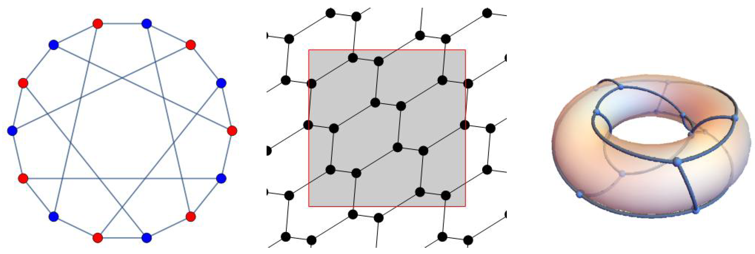
Here, ${\mathbb{F}}_2$ is the finite field with 2 elements. The automorphism group of $\mathcal{X}$ contains the group PGL${}_2\left({\mathbb{F}}_2\right)$ as an index two subgroup of order 168. The spectrum of the Laplacian of $\mathcal{X}$ is

$$0<\underset{6-\mathrm{times}}{\underbrace{(3-\sqrt{2})=\cdots =(3-\sqrt{2})}}<\underset{6-\mathrm{times}}{\underbrace{(3+\sqrt{2})=\cdots =(3+\sqrt{2})}}<6.$$

Let $\sigma =\left(\begin{array}{ccc}0& 0& 1\\ 1& 0& 1\\ 0& 1& 0\end{array}\right)$ which is an element of order 7 in PGL${}_2\left({\mathbb{F}}_2\right)$. Choose $W_1$ and $W_2$ to be two orthogonal rotational planes of ${\rho }_{\sigma }$ in the 6-dimensional subspace $E(3-\sqrt{2})$. In this case, the result drawing of the Heawood graph $\mathcal{X}$ gives an embedding on a torus as shown in Figure 7.

Example 5.

Let $\mathcal{X}=G(n,k)$ be the generalized Petersen graph which vertex set is $\{u_1$$,\cdots$, $u_n$, $v_1,\cdots ,v_n\}$ and the edge is ${\bigcup }_{i=1}^n\{(u_i,u_{i+1}),(u_i,v_i),(v_i,v_{i+k})\}$ were subscripts are to be read modulo n. Let σ be the automorphism on $\mathcal{X}$ given by $\sigma \left(v_i\right)=v_{i+1}$ and $\sigma \left(u_i\right)=u_{i+1}$ for all i. There are three torodial edge-transitive petersen graphs, namely the Petersen graph $G(5,2)$, the Möbius–Kantor graph $G(8,3)$, and the Nauru graph $G(12,5)$.

1. 

For the Petersen graph $G(5,2)$, the second smallest eigenvalue ${\lambda }_2$ of the Laplacian equals 2, which is of dimension 5. Let $W_1$ and $W_2$ be two rotational planes of ${\rho }_{\sigma }$ on $E\left({\lambda }_2\right)$. However, in the resulted drawing as shown in Figure 8, 10 vertices are divided into 5 pairs and each pair maps to one point.

2. 

For the Möbius–Kantor graph $G(8,3)$, the second smallest eigenvalue ${\lambda }_2$ of the Laplacian equals $3-\sqrt{3}$, which is of dimension 4. Let $W_1$ and $W_2$ be two rotational planes of σ on $E\left({\lambda }_2\right)$. However, in the resulted drawing as shown in Figure 9, 16 vertices are divided into 8 pairs and each pair maps to one point.

3. 

For the Nauru graph $G(12,5)$, the second smallest eigenvalue ${\lambda }_2$ of the Laplacian equals $3-\sqrt{3}$, which is of dimension 4. Let $W_1$ and $W_2$ be two rotational planes of σ on $E\left({\lambda }_2\right)$. However, in the resulted drawing as shown in Figure 10, 24 vertices are divided into 12 pairs and each pair maps to one point.

For torodial generalized Petersen graphs and this particular σ, our algorithm does not give an embedding onto a torus. One may choose a different σ to obtain a different drawing. However, unlike other examples, none of σ induces an embedding onto a torus.

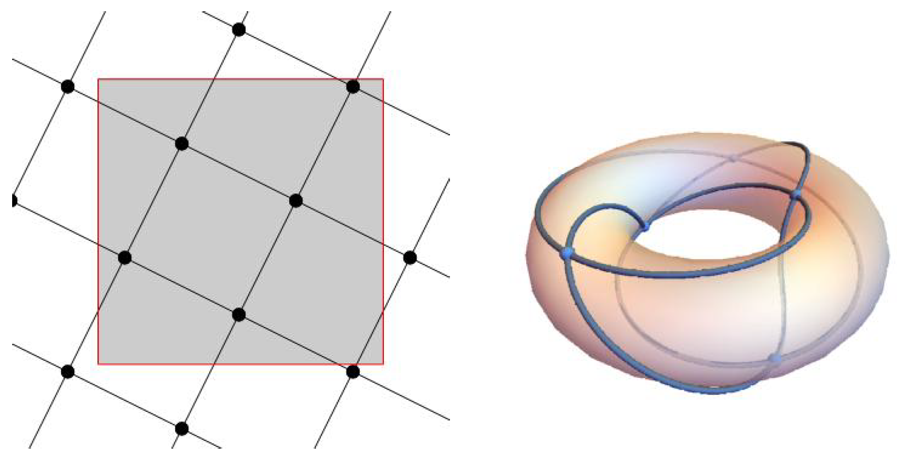
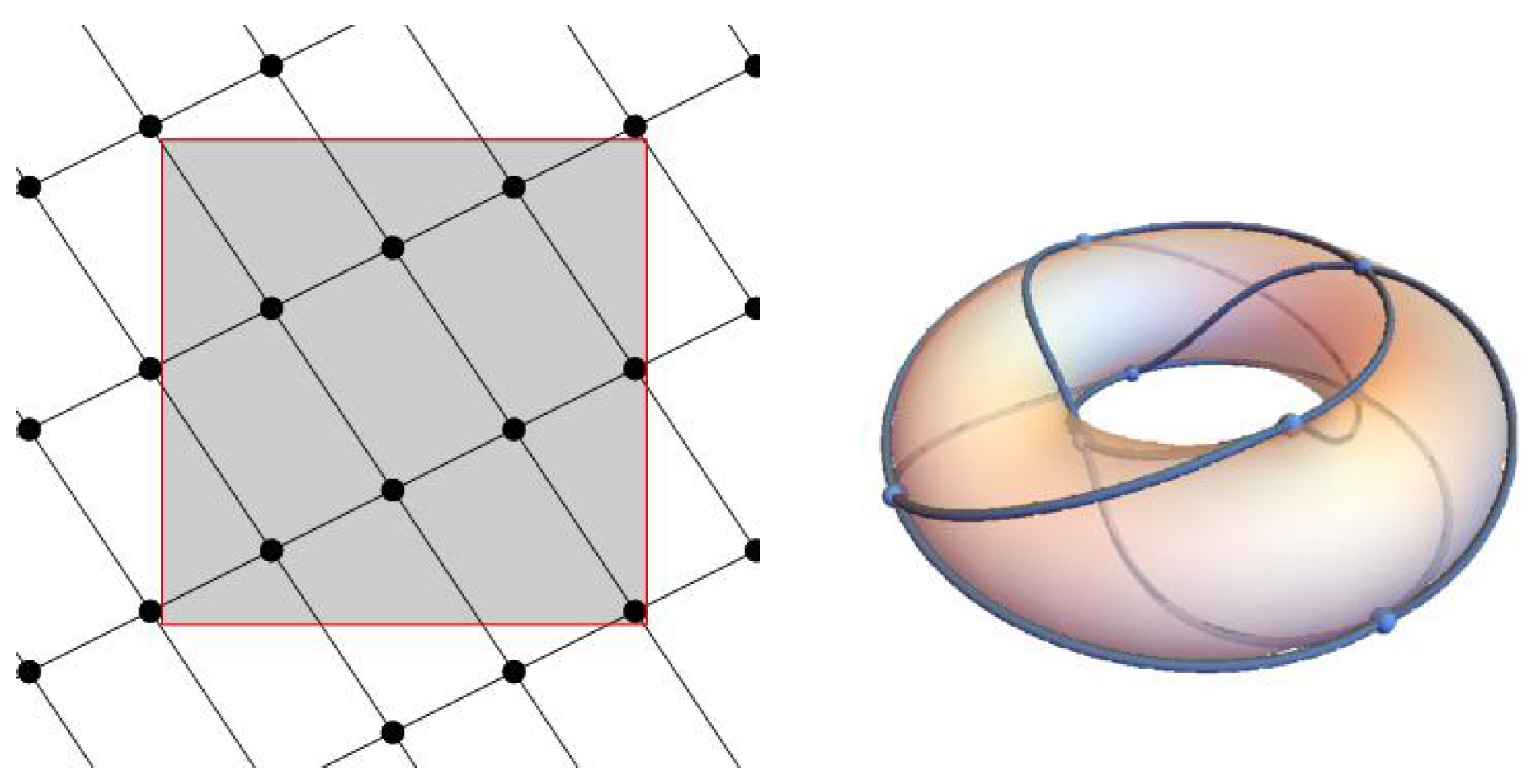
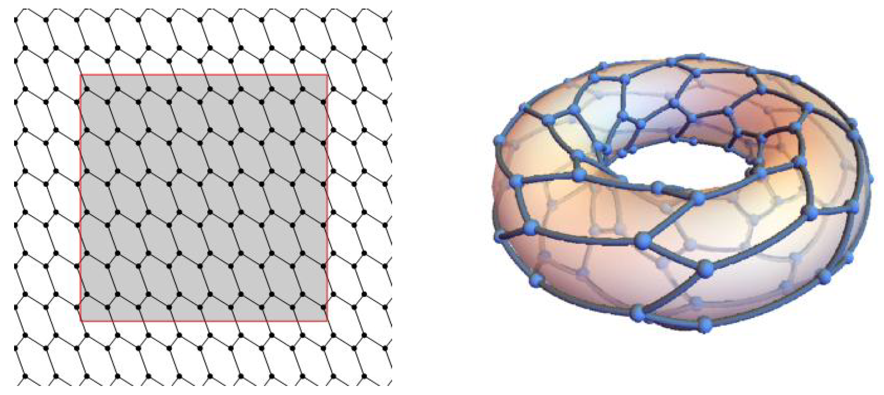
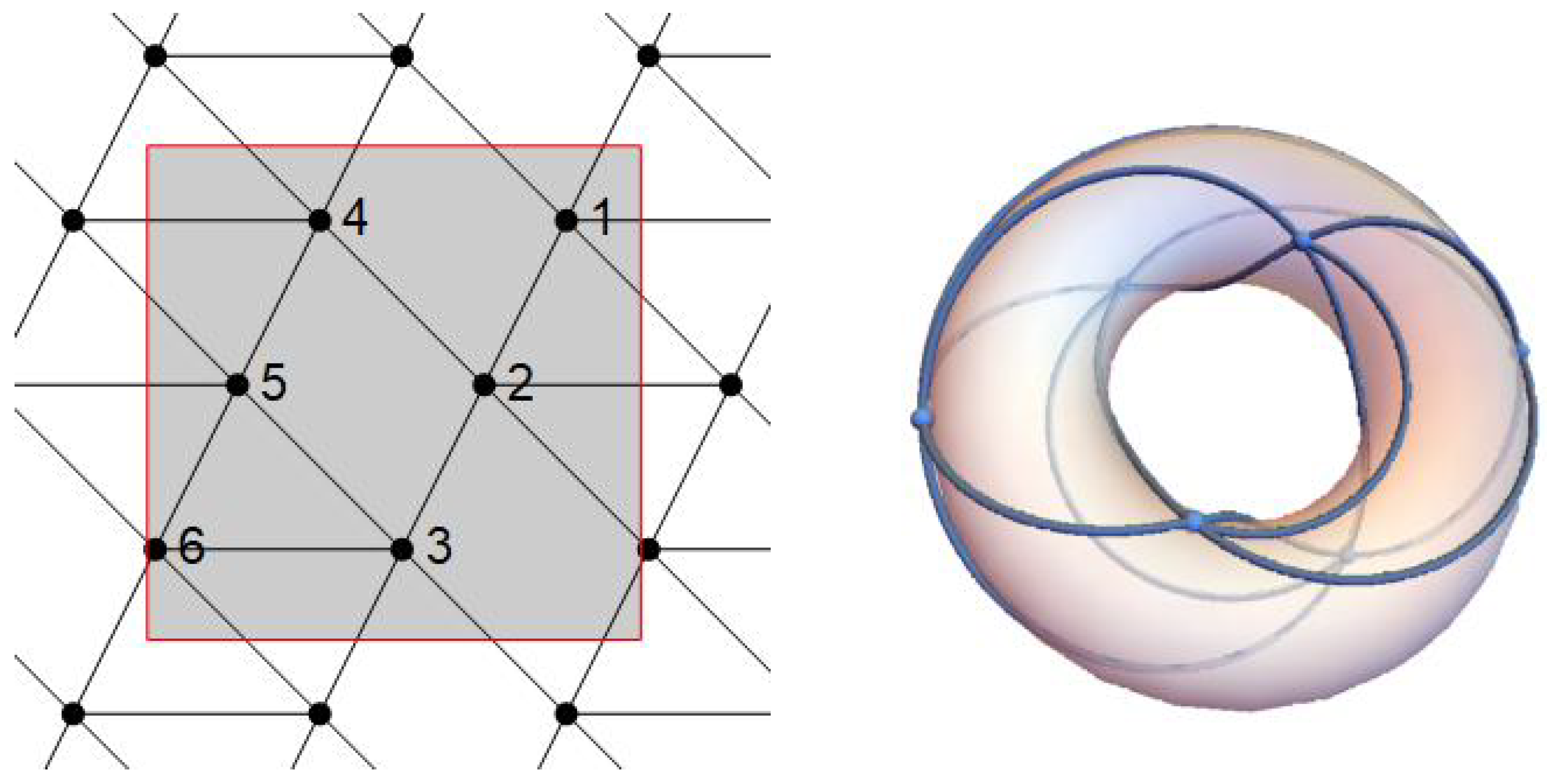
Example 6.

Let $G=\mathbb{Z}/m\mathbb{Z}\times \mathbb{Z}/n\mathbb{Z}$ and $S=\left\{(\pm 1,\pm 1)\right\}$. The Cayley graph $\mathcal{X}$ of $(G,S)$ is a rectangular mesh on a torus. The spectrum of the Laplacian L is given by

$$\left\{4-2cos\left(\frac{2\pi j}{m}\right)-2cos\left(\frac{2\pi k}{n}\right)|1\le j\le m,1\le k\le n\right\}.$$

When $n\ne m$, we have

$$0={\lambda }_1<{\lambda }_2={\lambda }_3<{\lambda }_4={\lambda }_5<{\lambda }_6.$$

In this case, we can simply set $W_1=E\left({\lambda }_2\right)$ and $W_2=E\left({\lambda }_4\right)$ and the result drawing of the Cayley graph X gives an embedding on a torus as shown in Figure 11.

When $n=m$, we have

$$0={\lambda }_1<{\lambda }_2={\lambda }_3={\lambda }_4={\lambda }_5<{\lambda }_6.$$

Set $\sigma \left(x\right)=x+(1,2).$ In this case, $E\left({\lambda }_2\right)$ can be decomposed as a direct sum of two orthogonal rotational planes $W_1$ and $W_2$ of ${\rho }_{\sigma }$. In this case, the result drawing of the Cayley graph X gives an embedding on a torus as shown in Figure 12.

Note that the symmetric drawing of the Cayley graph in this example has been studied in the 3-sphere in [9,10].

Example 7.

Let G be a group of isometries on ${\mathbb{R}}^2$ generated by three isometries:

$$s_1\left(\overrightarrow{x}\right)=-\overrightarrow{x}+(1,0),s_2\left(\overrightarrow{x}\right)=-\overrightarrow{x}+(0,1),and s_3\left(\overrightarrow{x}\right)=-\overrightarrow{x}+(1,1).$$

Let N be a translation subgroup spanned by $t_1\left(\overrightarrow{x}\right):=\overrightarrow{x}+{\overrightarrow{u}}_1$ and $t_1\left(\overrightarrow{x}\right)=\overrightarrow{x}+{\overrightarrow{u}}_2$ for some ${\overrightarrow{u}}_1,{\overrightarrow{u}}_2\in {\mathbb{Z}}^2$. In this case N is a normal subgroup of G and the Cayley graph $\mathcal{X}$ of $(G/N,\{s_1,s_2,s_3\})$ is a so-called toroidal fullerence. The spectrum of the Laplacian can be found in [11] Especially, when ${\overrightarrow{u}}_1=(m,0)$ and ${\overrightarrow{u}}_2=(0,n)$, the spectrum of the Laplacian is given by

$$\{3\pm \sqrt{3+2cos(2\pi j/m)+2cos(2\pi k/n)+2cos\left(2\pi \right(j/m+k/n\left)\right)}|1\le j\le m,1\le k\le n\}.$$

When $n=m$, we have

$$0={\lambda }_1<{\lambda }_2={\lambda }_3={\lambda }_4={\lambda }_5={\lambda }_6={\lambda }_7<{\lambda }_8.$$

Set $\sigma \left(x\right)=x+\overline{(1,2)}.$ In this case, the six dimensional subspace $E\left({\lambda }_2\right)$ can be decomposed as a direct sum of three rotational planes of ${\rho }_{\sigma }$. We choose $W_1$ and $W_2$ as any two of them. In this case, the result drawing of the Cayley graph X gives an embedding on a torus as shown in Figure 13.

When $n\ne m$, we have

$$0={\lambda }_1<{\lambda }_2={\lambda }_3<{\lambda }_4={\lambda }_5<{\lambda }_6.$$

In this case, we can simply set $W_1=E\left({\lambda }_2\right)$ and $W_2=E\left({\lambda }_4\right)$ and the result drawing of the Cayley graph X gives an embedding on a torus as shown in Figure 14.

4. Further Works

In this paper, we provide a simple algorithm to draw torodial graphs on three-dimensional Euclidean space. The main idea is to express the torus as a product of two 1-spheres $S^1\times S^1$, which can be regarded a subset of $S^3$.

However, our method can not apply to graphs of high genus since there is no simple way to describe closed surfaces of high genus in three-dimensional Euclidean space.

In the future, we would like to study graphs of genus two as the starting point. Such graphs shall be drawn on the so-called double torus. Unlike the usual torus, the double torus is a quotient of the hyperbolic plane. Therefore, the a new method must be developed.

References

- Gross, J.L.; Insel, T.; Thomas, W. An r-Dimensional Quadratic Placement Algorithm. Manag. Sci. 1970, 17, 219–229. [Google Scholar]
- Koren, Y. On spectral graph drawing. In International Computing and Combinatorics Conference; Lecture Notes in Computer Science; Springer: Berlin, Germany, 2003; Volume 2697, pp. 496–508. [Google Scholar]
- Gross, J.L.; Tucker, T.W. Topological Graph Theory, Wiley-Interscience Series in Discrete Mathematics and Optimization; John Wiley & Sons, Inc.: New York, NY, USA, 1987. [Google Scholar]
- Holton, D.A.; Sheehan, J. The Petersen Graph, Australian Mathematical Society Lecture Series; Cambridge University Press: Cambridge, UK, 1993; Volume 7. [Google Scholar]
- Aleardi, L.C.; Devillers, O.; Fusy, E. Canonical ordering for graphs on the cylinder, with applications to periodic straight-line drawings on the flat cylinder and torus. J. Comput. Geom. 2018, 9, 391–429. [Google Scholar]
- Kocay, W.; Neilson, D.; Szypowski, R. Drawing graphs on the torus. Ars Combin. 2001, 59, 259–277. [Google Scholar]
- Kocay, W.; Neilson, D.; Szypowski, R. Embeddings of Small Graphs on the Torus. Cubo Mater. Educ. 2003, 5, 351–371. [Google Scholar]
- Friedberg, S.H.; Insel, A.J.; Spence, L.E. Linear Algebra; Prentice Hall, Inc.: Upper Saddle River, NJ, USA, 2018. [Google Scholar]
- Lawrencenko, S. Geometric realization of toroidal quadrangulations without hidden symmetries. Ceombinatorices 2014, 1, 11–20. [Google Scholar]
- Lawrencenko, S.; Shchikanov, A.Y. Euclidean realization of the product of cycles without hidden symmetries. Sib. Èlektron. Mater. Izv. 2015, 12, 777–783. (In Russian) [Google Scholar]
- Kang, M.-H. Toroidal fullerenes with the Cayley graph structures. Discrete Math. 2011, 311, 2384–2395. [Google Scholar] [CrossRef] [Green Version]