Article

An Effective Approximation Algorithm for Second-Order Singular Functional Differential Equations

1
Department of Applied Mathematics, Faculty of Mathematics and Computer, Shahid Bahonar University of Kerman, Kerman 76169-14111, Iran
2
Department of Mathematics and Statistics, University of Victoria, Victoria, BC V8W 3R4, Canada
3
Department of Medical Research, China Medical University Hospital, China Medical University, Taichung 40402, Taiwan
4
Department of Mathematics and Informatics, Azerbaijan University, 71 Jeyhun Hajibeyli Street, AZ1007 Baku, Azerbaijan
5
Section of Mathematics, International Telematic University Uninettuno, I-00186 Rome, Italy
6
Department of Mathematics and Engineering Physics, Faculty of Engineering, Mansoura University, Mansoura 35516, Egypt
7
Faculty of Engineering, Université Française d’Egypte, Ismailia Desert Road, El Shorouk, Cairo, Egypt
*
Author to whom correspondence should be addressed.
Axioms 2022, 11(3), 133; https://doi.org/10.3390/axioms11030133
Submission received: 22 February 2022 / Revised: 11 March 2022 / Accepted: 12 March 2022 / Published: 14 March 2022
(This article belongs to the Special Issue Mathematical Analysis and Applications III)

Abstract

:
In this research study, a novel computational algorithm for solving a second-order singular functional differential equation as a generalization of the well-known Lane–Emden and differential-difference equations is presented by using the Bessel bases. This technique depends on transforming the problem into a system of algebraic equations and by solving this system the unknown Bessel coefficients are determined and the solution will be known. The method is tested on several test examples and proves to provide accurate results as compared to other existing methods from the literature. The simplicity and robustness of the proposed technique drive us to investigate more of their applications to several similar problems in the future.

1. Introduction

The primary concern of this research work is to develop a computationally effective technique, which relies on novel Bessel polynomials and a set of collocation points to find the solutions of the following second-order singular functional differential equations (SFDEs)
d 2 d x 2 w ( a x + b ) + μ x d d x w ( c x + d ) + r ( x ) w ( e x + f ) = p ( x ) , 0 < x ,
where the constants a , b , c , d , e , f , and μ are in R . Moreover, is a positive real number and r ( x ) , p ( x ) are given real-valued functions. The above SFDEs are accompanied with the initial conditions
w ( 0 ) = w 0 , d d x w ( 0 ) = w 1 .
The study of the singular functional differential equations (SFDEs) is one of the most important areas of study with a variety of applications in engineering and science topics. The researcher community is continuously investigating the possible applications of these types of equations and numerous fields are reported including electrodynamics [1], models of infectious diseases [2], population growth models [3], the simulation of tumor growth [4], the processing of chemical systems [5], understanding the gene system [6], and viral infectious models [7]. These models have attracted the attention of many scientists with their singularity at the origin or other points. One of the most important models that has this type of equation is the well-known Lane–Emden type equations (LEE) that have been used since they was named after the famous astrophysicists Jonathan Homer Lane and Robert Emden back in 1870. The Lane–Emden equations have some applications in the field of models of thermal explosion [8], models of isothermal gas spheres [9], stellar structure [10], and the study of thermionic current. These potential and important applications have motivated researchers to investigate the solution of these models more.
Finding the approximate solution of the LEE is one of the most interesting subjects for scientists and researchers. For obtaining the results for the solutions of these types of problems, some numerical and analytical techniques have been adapted, acquiring good results. For example, Mirazaee et al. in [11] investigated a Fibonacci polynomials based method for solving this problem. Moreover, Kadalbajoo et al. [12] adapted a method with Taylor series expansion for solving a similar type of equation. The asymptotic solutions are analyzed in [13] for a class of nonlinear singular perturbed equations. Sabir et al. [14] performed a neuro-swarm intelligent computing algorithm for solving a second-order type equation. Other reported methods can be found in [15,16,17,18,19] and references therein with multiple other applications of this problem. All of the above-mentioned methods, either analytical or numerical, have some advantages and disadvantages in terms of errors or computational costs. Thus, we searched for a suitable collocation based method to adapt and acquire more accurate results which urges us to use the Bessel collocation method.
The appearance of new Bessel functions related to the Bessel functions of the first type was systematically shown in a seminal paper [20]. Since then, many research papers have been devoted to discovering many characteristics of these polynomials from the algebraic point of view; for more details, see [20,21,22,23,24,25,26]. In recent years, the study of different models with the aid of these polynomials has witnessed a large increase of research due to their simplicity and the ability to provide good results. For the recent applications of the Bessel polynomials, we draw your attention to some recent works we have done in [27,28,29]. The main goal of this research work is to propose a spectral approach based on a combination of novel Bessel bases as well as some appropriate collocation points for an approximate treatment of the SFDEs in (1). Supposedly, the underlying model problem has a solution in terms of the Bessel series expansion on [ 0 , ] , the proper representations of the unknowns and their derivatives yield to find the unknown series coefficients, through solving an algebraic system of equations. Indeed, the explicit and original representation of the Bessel functions is
B m ( ξ ) = σ = 0 m 2 σ ( m + σ ) ! σ ! ( m σ ) ! ξ σ , m = 0 , 1 , .
It can be obviously observed that the coefficients of B m ( ξ ) are all positive. Contrary to the Bessel functions of the first kind [30], the novel Bessel functions B m ( ξ ) are the unique solutions of the following differential equation [27,28,29]
ξ 2 B m ( ξ ) + ( 2 ξ + 2 ) B m ( ξ ) = m ( m + 1 ) B m ( ξ ) .
The main capability of of the proposed Bessel spectral algorithm is that it converts the SFDEs (1) to a system of algebraic equations while reducing computational complexity. Usages of the proposed technique but with different bases such as Legendre, Chebyshev, Chelyshkov, alternative Bessel, and Jacobi functions can be found in [31,32,33,34,35,36,37,38,39,40].
The outline of this study is structured as follows. The next section provides the methodology of the Bessel matrix procedure for the SFDEs in an elegant manner. In Section 3, three test examples are solved in order to evaluate the reliability and accuracy of the presented matrix technique. In Section 4, we present a summary and conclusion.

2. The Bessel Matrix Technique

In order to utilize the Bessel functions on [ 0 , ] , we first make a change of variable in (3). We take ξ = x / where > 0 in (3). Henceforth, the shifted Bessel functions will be denoted by B m , ( x ) , which are orthogonal with respect to g ( x ) : = e x p ( 2 / x ) ; see [20,27]. Suppose that the unknown solution w ( x ) of (1) can be expanded in the Bessel polynomials form
w N ( x ) = m = 0 N c m B m , ( x ) , 0 x .
Now, the ultimate goal is to seek the coefficients c m for m = 0 , 1 , , N . To proceed, we introduce the unknown vector
C N = [ c 0 c 1 c N ] T ,
and the vector containing the shifted Bessel functions of order m = 0 to m = N as
V N ( x ) = B 0 , ( x ) B 1 , ( x ) B N , ( x ) .
Thus, on the other hand, we have the following expression for w N ( x ) in (4) in the form
w N ( x ) = V N ( x ) C N .
Next, we introduce the following Bessel matrix L, which has a low-triangular structure and is of size ( N + 1 ) × ( N + 1 )
L = 1 0 0 0 0 1 1 0 0 0 1 3 3 0 0 1 2 1 N ! 1 ( N 2 ) ! 1 ! 2 2 ( N + 1 ) ! 2 ( N 3 ) ! 2 ! 2 1 N ( 2 N 2 ) ! N 1 0 ! ( N 1 ) ! 0 1 2 1 ( N + 1 ) ! 1 ( N 1 ) ! 1 ! 2 2 ( N + 2 ) ! 2 ( N 2 ) ! 2 ! 2 1 N ( 2 N 1 ) ! N 1 1 ! ( N 1 ) ! 2 N ( 2 N ) ! N 0 ! N ! ( N + 1 ) × ( N + 1 ) .
This allows us to write further the vector V N ( x ) in (5) in the product representation form
V N ( x ) = Ξ N ( x ) L T ,
where Ξ N ( x ) = 1 x x 2 x N stands for the vector of monomials.
Finally, we place relation (6) into (5) to arrive at the following form of approximate solution w N ( x ) in (4) as
w N ( x ) = V N ( x ) C N = Ξ N ( x ) L T C N .
We now mention a pertinent result about the convergence of Bessel functions. The following theorem asserts that the approximate solution w N ( x ) is exponentially convergent (in the weighed L 2 norm) to the exact solution w ( x ) if we let N tend to infinity.
Theorem 1.
Let us denote by w N ( x ) = V N ( x ) C N the best square approximation to w ( x ) and also we have w ( x ) C N + 1 ( 0 , ] . Then, the following error estimate holds
w ( x ) w N ( x ) g N + 3 2 2 N + 3 e 1 K ( N + 1 ) ! ,
where K : = max x ( 0 , ] | w ( N + 1 ) ( x ) | .
Proof. 
For a similar proof, we refer interested readers to [27,30].    □
We now associate a sequence of collocation points { x q } q = 0 N on [ 0 , ] to our approximation algorithm. In this respect, the following grid points are employed
x q = ξ + ( ξ ) q N , q = 0 , 1 , , N , 0 < ξ < .
Once the preceding collocation points are placed into the relation (7), we get the matrix expression for the unknown solution itself as
W = χ L T C N , χ = Ξ N ( x 0 ) Ξ N ( x 1 ) Ξ M ( x N ) , W = w N ( x 0 ) w N ( x 1 ) w N ( x N ) .
In order to express w ( α x + β ) and its derivatives in the matrix forms, we state and prove the next theorem.
Theorem 2.
For any constants α and β, the matrix representations of w ( α x + β ) , d d x w ( α x + β ) , and d 2 d x 2 w ( α x + β ) at the collocation points (8) can be represented as
W α , β = χ H α , β T L T C N ,
W ˙ α , β = χ H α , β T B T L T C N ,
W ¨ α , β = χ H α , β T ( B T ) 2 L T C N .
Here, the matrix B is defined in (15) and the matrix H α , β is given at (14). Moreover, we have
W α , β = w N ( α x 0 + β ) w N ( α x 1 + β ) w N ( α x N + β ) , W ˙ α , β = w N ( α x 0 + β ) w N ( α x 1 + β ) w N ( α x N + β ) , W ¨ α , β = w N ( α x 0 + β ) w N ( α x 1 + β ) w N ( α x N + β ) .
Proof. 
According to (7), we may write
w N ( α x + β ) = Ξ N ( α x + β ) L T C N .
Our aim is to express Ξ N ( α x + β ) in terms of Ξ N ( x ) , which is defined in (6). With the help of the binomial expansion,
( α x + β ) n = j = 0 n n j α j β n j x j ,
we can represent the vector Ξ N ( α x + β ) as follows
Ξ N ( α x + β ) = Ξ N ( x ) H α , β T ,
where the matrix H α , β T is dependent on two parameters α and β and is defined as
H α , β T = 0 0 α 0 β 0 1 0 α 0 β 1 2 0 α 0 β 2 N 0 α 0 β N 0 1 1 α 1 β 0 2 1 α 1 β 1 N 1 α 1 β N 1 0 0 2 2 α 2 β 0 N 2 α 2 β N 2 0 0 0 N N α N β 0 .
Now, we combine the relations (13) and (14) to obtain
w N ( α x + β ) = Ξ N ( x ) H α , β T L T C N .
We are now ready to put the collocation points (8) into the preceding equation followed by utilizing the relation (9); the proof of (10) is done.
We then find a relationship between Ξ N ( x ) and d s d x s Ξ N ( x ) for s = 1 , 2 . For this purpose, we define the differentiation matrix B through defining
B T = 0 1 0 0 0 0 2 0 0 0 0 0 N 0 0 0 0 ( N + 1 ) × ( N + 1 ) .
It can be easily seen that [30]
d d x Ξ N ( x ) = Ξ N ( x ) B T ,
Differentiating the relation (15) once more, we get
d 2 d x 2 Ξ N ( x ) = Ξ N ( x ) ( B T ) 2 .
Our next aim is to differentiate (7) with respect to the variable x and utilize (15). Therefore, we will get the following approximation for d d x w N ( α x + β ) as
d d x w N ( α x + β ) d d x w N ( x ) | x ( α x + β ) = Ξ N ( x ) | x ( α x + β ) B T L T C N .
In the same manner, after using (16) we get an approximation for d 2 d x 2 w N ( α x + β ) as follows
d 2 d x 2 w N ( α x + β ) d 2 d x 2 w N ( x ) | x ( α x + β ) = Ξ N ( x ) | x ( α x + β ) ( B T ) 2 L T C N .
We now replace the vector Ξ N ( α x + β ) in (17) and (18) via (14). Thus, we get the following matrix representation forms
d d x w N ( α x + β ) = Ξ N ( x ) H α , β T B T L T C N , d 2 d x 2 w N ( α x + β ) = Ξ N ( x ) H α , β T ( B T ) 2 L T C N .
The proofs of (11) and (12) are straightforward after inserting the collocation points (8) into the foregoing (19).    □
Remark 1.
It is worth mentioning the cost of calculating Ξ N ( α x + β ) as well as d s d x s Ξ N ( α x + β ) for s = 1 , 2 in (19) is O ( ( N + 1 ) 2 ) . For practical applications, however, it would be very useful to consider an algorithm with linear complexity O ( N + 1 ) . This task can be accomplished by taking direct differentiation of the monomials Ξ N ( x ) . Upon calling Algorithm 1, the s-order derivatives ( s 1 , s N ) of Ξ N ( x ) can be achieved directly. Let us assume that Algorithm 1 takes ( N = 4 , s ) as inputs. The outputs with s = 1 and s = 2 are as follows, respectively:
d d x Ξ 4 ( x ) = 0 1 2 x 3 x 2 4 x 3 , d 2 d x 2 Ξ 4 ( x ) = 0 0 2 6 x 12 x 2 .
In this work, we are particularly interested in computing the first and second derivatives of Ξ N ( x ) by Algorithm 1. This enables us to compute d s d x s Ξ N ( α x + β ) for s = 0 , 1 , 2 after invoking Algorithm 1 followed by substituting x ( α x + β ) in them.
Algorithm 1: The computation of s-derivative of the vector Ξ N ( x ) .
  • procedure [ Ξ N ( s ) ] = compute_DerX ( N , s )
  • Ξ N ( s ) [ 1 ] : = 0 ;
  • for j : = 1 , , N do
  • if ( j s < 0 ) then
  •    Ξ N ( s ) [ j + 1 ] : = 0 ;
  • else
  •    ( ( Ξ N ( s ) [ j + 1 ] : = j ! ( j s ) ! x j s ;
  • end if
  • end for
  • end;
The considered SFDE problem (1) will be collocated at the set of collocation points (8) to arrive at
d 2 d x 2 w ( a x q + b ) + μ x q d d x w ( c x q + d ) + r ( x q ) w ( e x q + f ) = p ( x q ) , q = 0 , 1 , , N .
To express the former N + 1 equations in a matrix representation, we exploit the results of Theorem 2 to have
W ¨ a , b + Q W ˙ c , d + R W e , f = P .
Two matrices Q , R and the vector P are
Q = μ x 0 0 0 0 μ x 1 0 0 0 μ x N , R = r ( x 0 ) 0 0 0 r ( x 1 ) 0 0 0 r ( x N ) , P = p ( x 0 ) p ( x 1 ) p ( x N ) , ,
We finally obtain the so-called fundamental matrix equation for the underlying model (1).
Lemma 1.
Suppose that the solution of model problem (1) can be expanded in Bessel function form (4) or (7). Then we have
χ H a , b T ( B T ) 2 + Q χ H c , d T B T + R χ H e , f T L T Z C N = P , o r [ Z ; P ] .
Proof. 
To conclude the fundamental matrix Equation (23), it is sufficient to place relations (10), (11), and (12) into (21). □
Let us emphasize that the algebraic matrix Equation (23) is linear and the unknown coefficient C N can be calculated through solving it. However, the initial conditions (2) must be utilized in implementation of the fundamental matrix Equation (23). This aim will be considered below.

Initial Conditions in the Matrix Form

Analogously, we are able to approximate the initial conditions (2) in the matrix form, which allows us to find the solution of (1) via solving the fundamental matrix Equation (23). We first convert w ( 0 ) = w 0 into a matrix representation. To this end, let us tend t 0 in (7) to arrive at
Z ^ 0 : = Ξ N ( 0 ) L T C N = w 0 , or [ Z ^ 0 ; w 0 ] .
For the second condition d d x w ( 0 ) = w 1 , we first differentiate (7). Hence, we combine the resultant equation with (15) to get
d d x w N ( x ) = d d x Ξ N ( x ) L T C N = Ξ N ( x ) B T L T C N .
Now, let t 0 in the foregoing equation to obtain
Z ^ 1 : = Ξ N ( 0 ) B T L T C N = w 1 , or [ Z ^ 1 ; w 1 ] .
Now, to the fundamental matrix Equation (23), we add the initial conditions (2). For this purpose, the replacements of the first and the second row of the matrix [ Z ; P ] are done by the row matrices [ Z ^ 0 ; w 0 ] and [ Z ^ 1 ; w 1 ] . Let us denote by [ Z ^ ; P ^ ] the modified version of the fundamental matrix. After solving this modified form, the unknown coefficients c m , m = 0 , 1 , , N will be calculated and thus the desired approximation w N ( x ) of SFDEs (1) will be determined.

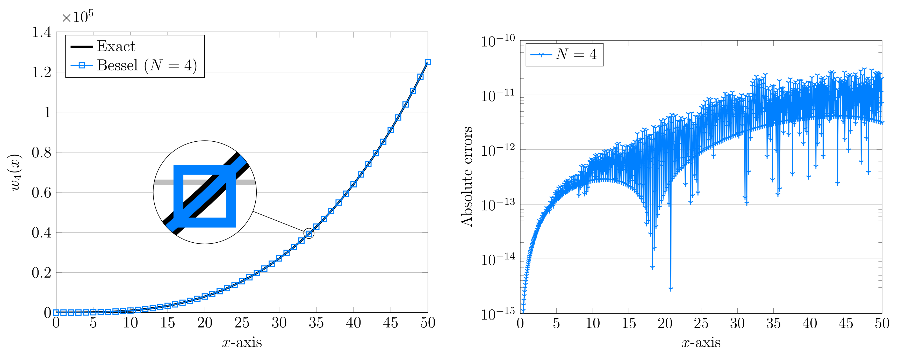
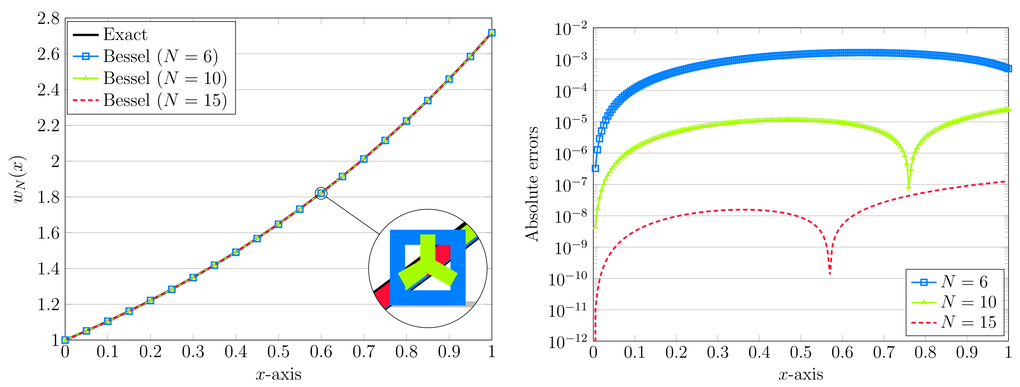
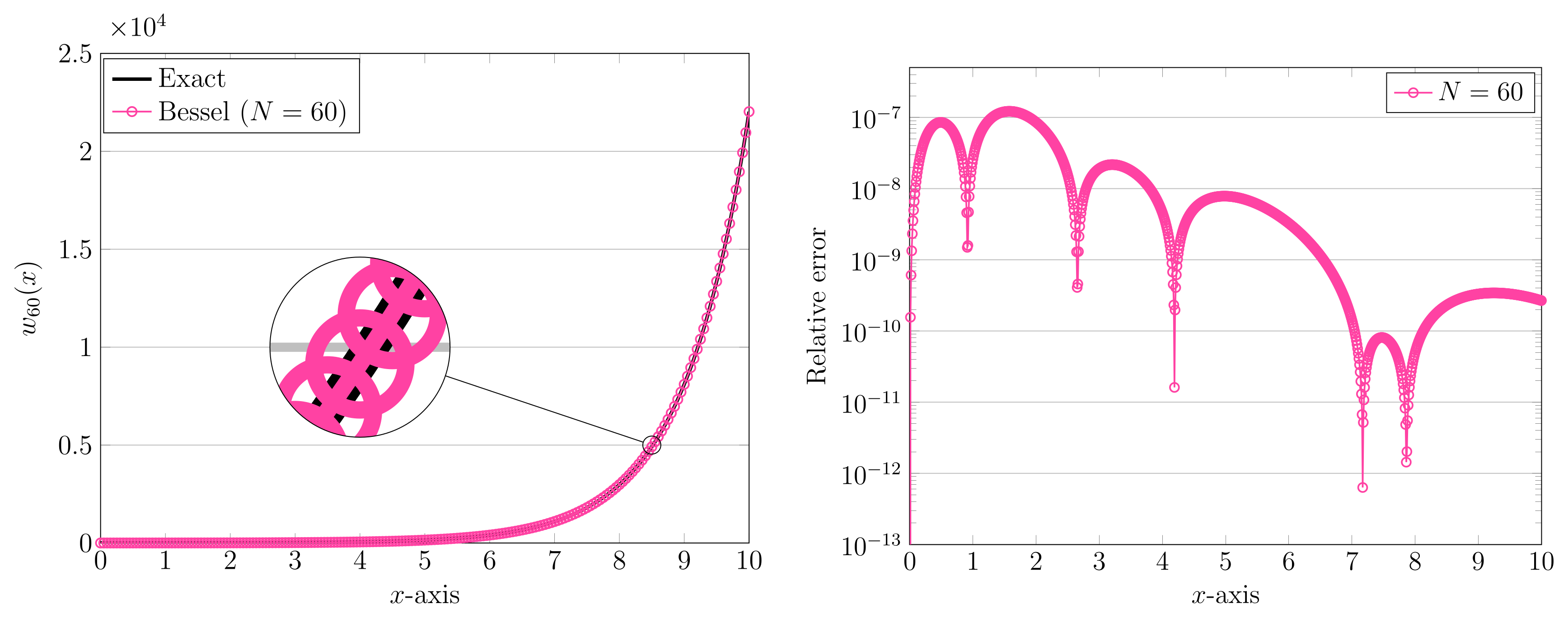
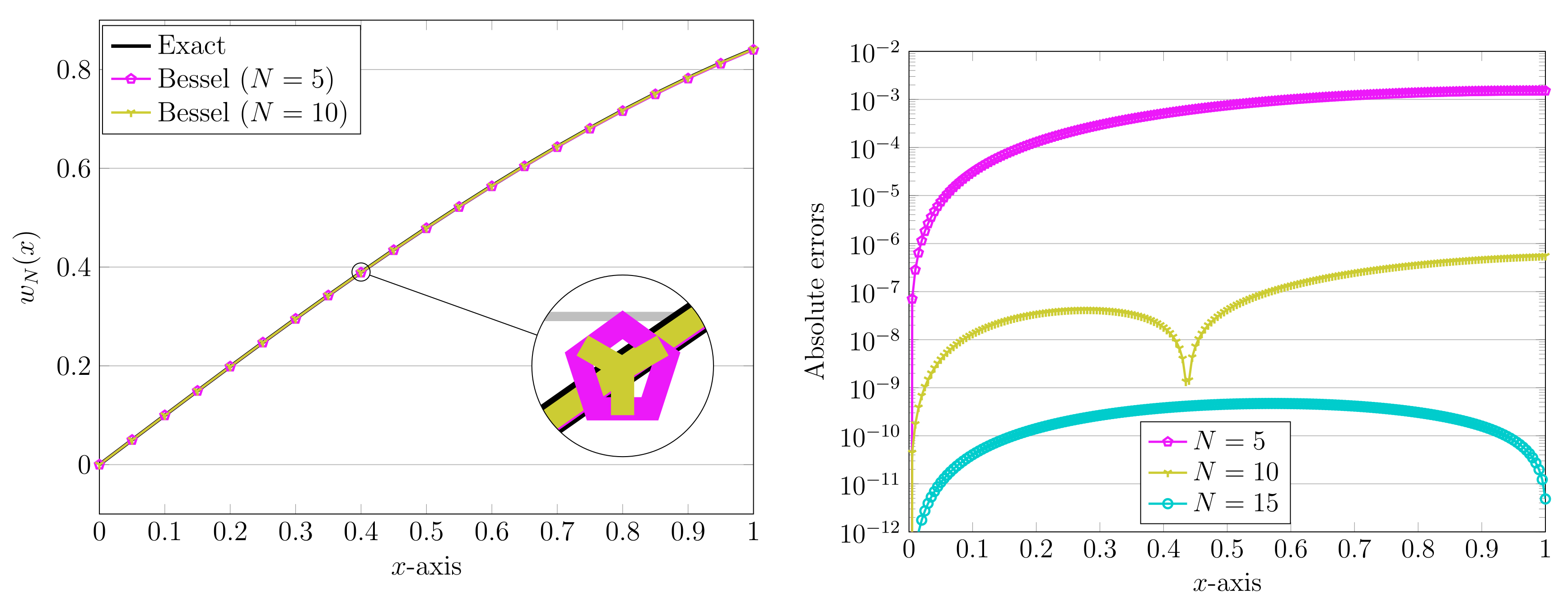
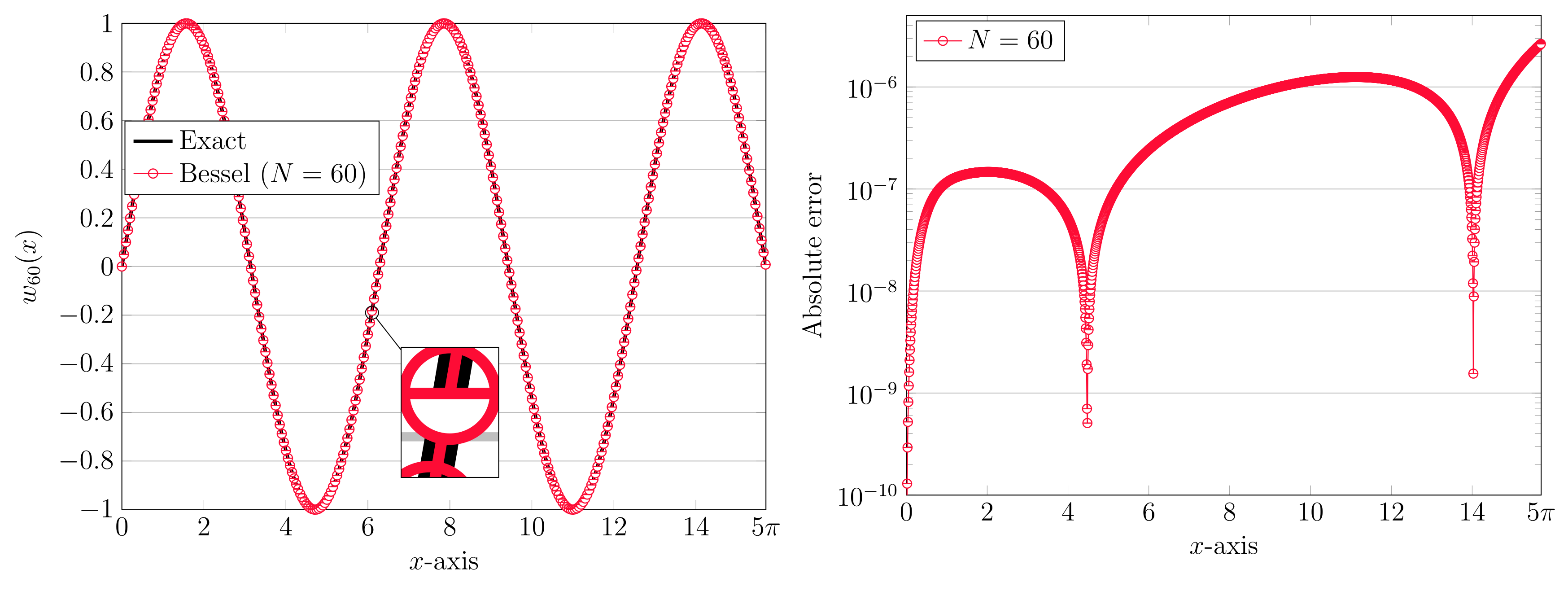
3. Computational Simulations

Let us illustrate the practicability of our Bessel matrix approach through numerical simulations. In this respect, computational results of three test examples are performed to show the reliability and validity of the proposed numerical model. Thus, we show that our suggested approximation algorithm can produce improved results compared to existing available computational procedures. For numerical simulations, we use MATlAB software version 2017a for programming and visualization. Moreover, the value ξ = 0.01 is taken in the set of collocation points (8) in order to ensure that the zero point is excluded from this set. In order to evaluate the accuracy as well as the convergence of the proposed Bessel matrix technique, we define
E N ( x ) : = | w N ( x ) w ( x ) | , x [ 0 , ] , R N ( x ) : = E N ( x ) / | w ( x ) | , x [ 0 , ] .
Example 1.
We firstly consider a non-homogeneous singular differential difference model problem of the form
d 2 d x 2 w ( 3 x 1 ) + 2 x d d x w ( 2 x ) + x w ( x + 1 ) = 6 + 44 x + 3 x 2 + 3 x 3 + x 4 , 0 x ,
with initial conditions w ( 0 ) = 1 , d d x w ( 0 ) = 0 . A straightforward calculation shows that true exact solution is given by w ( x ) = 1 + x 3 .
For this test problem, we set = 10 , and utilize N = 3 , which is sufficient to obtain an accurate solution. To do so, we express the solution of (1) in terms of Bessel bases as considered in (4). Afterwards, through solving the fundamental matrix Equation (23), we obtain
C 3 = 997 / 3 600 1000 / 3 200 / 3 T .
By exploiting the first four Bessel basis functions and multiply them by C 3 , we get the approximate solution w 3 ( x ) on 0 x 10 as follows
w 3 ( x ) = 1 B 1 , ( x ) B 2 , ( x ) B 3 , ( x ) C 3 = 1 + x 3 .
Clearly this is the exact solution of (1). In the next experiments, the results of absolute errors utilizing diverse values of = 1 , 5 , 20 are computed. Table 1 tabulates the results of E N ( x ) which are calculated at some points x j = j / 10 and j varies from 1 to 10. A comparison with the outcomes of artificial neural networks (ANNs) reported in [17] on [ 0 , 1 ] and with 10 neurons is carried out in Table 1 to testify to the validity of our numerical results. An obvious conclusion can be made from Table 1 that our numerical model results are not only highly accurate on the unit interval but also have sufficient accuracy for the larger values of .
Utilizing = 1 , 5 , 20 , the obtained approximate solutions by the Bessel matrix approach are given by
w 3 ( x ) = 1.0 x 3 1.011761533 × 10 16 x 2 + 1.0 , x [ 0 , 1 ] , w 3 ( x ) = 1.0 x 3 2.43108357 × 10 15 x 2 5.450188595 × 10 107 x + 1.0 , x [ 0 , 5 ] , w 3 ( x ) = 1.0 x 3 + 3.669958207 × 10 15 x 2 + 1.0 , x [ 0 , 20 ] .
Finally, we consider N = 4 and = 50 for this example. The obtained approximate solution w 4 ( x ) for x [ 0 , ] takes the form
w 4 ( x ) = 7.132116273 × 10 18 x 4 + 1.0 x 3 7.257031883 × 10 15 x 2 3.966717388 × 10 105 x + 1.0 .
The above approximation together with the exact solutions are visualized in Figure 1. The resulting absolute errors are also presented in this figure, but on the right part.
Example 2.
As the second test problem, let us consider a Lane–Emden differential difference model problem of the form
d 2 d x 2 w ( 2 x 1 ) + 2 x d d x w ( 3 x ) + x w ( x + 1 ) = e 2 x 1 + 2 x e 3 x + x e x + 1 , 0 x ,
with initial conditions w ( 0 ) = 1 , d d x w ( 0 ) = 1 . It is not a difficult task to show that the exact solution of (2) is w ( x ) = e x .
Firstly, N = 6 is used for this example. Considering = 1 , the resulting approximate solution via the Bessel matrix technique takes the following form on x [ 0 , ]
w 6 ( x ) = 0.00464175985 x 6 0.001670260859 x 5 + 0.04740032168 x 4 + 0.1803886514 x 3 + 0.4870266818 x 2 + 1.0 x + 1.0 .
Let us check that our proposed method yields a reasonable result in comparison with the exact solution. In this respect, the first seven terms of its series expansion are written as
e x 1 + x + x 2 2 ! + x 3 3 ! + x 4 4 ! + x 5 5 ! + x 6 6 ! .
However, more accurate results based on the Bessel matrix approach will be achieved if one increases N. For instance, the approximated solution w 10 ( x ) can be analogous on [ 0 , 1 ] as
w 10 ( x ) = 0.000001068044011 x 10 0.000002908206541 x 9 + 0.00004176809694 x 8 + 0.0001888482682 x 7 + 0.001313363417 x 6 + 0.008508813772 x 5 + 0.04165172897 x 4 + 0.1663795908 x 3 + 0.5001750161 x 2 + 1.0 x + 1.0 .
Additionally, the graphical representation of the numerical results using different values of N = 6 , 10 and N = 15 are shown in Figure 2. In this plot, the absolute errors E N ( x ) for x [ 0 , 1 ] and for these values of N are also depicted.
In Table 2, the computed values of the values of the absolute errors E N ( x ) at some points x [ 0 , ] with = 1 , = 2 as well as = 5 for Example 2 are shown. The corresponding number of basis functions are N = 10 , 20 and N = 30 , respectively. Furthermore, the statistical results for this test example utilizing the ANN approach for = 1 and with 10 neurons that was proposed in [17] are reported in Table 2 for comparison.
In the next and last experiment performed for the test problem (2), we consider a relatively large domain of computation by choosing = 10 . To get a reasonable accuracy, we take N = 60 . In Figure 3, the curve of approximate solution w 60 ( x ) as well as the related relative error R N ( x ) are shown.
Example 3.
The last and third test case is devoted to the following singular differential difference with trigonometric functions defined on 0 x
d 2 d x 2 w ( 3 x 1 ) + 2 x d d x w ( 3 x ) + x w ( x + 1 ) = sin ( 3 x 1 ) + 2 x cos ( 3 x ) + x sin ( x + 1 ) ,
with initial conditions w ( 0 ) = 0 , d d x w ( 0 ) = 1 . An easy calculation shows that w ( x ) = sin x is the exact solution of this model problem.
Utilizing N = 5 , 10 in the Bessel matrix procedure, we get the following polynomial forms for the approximate solutions on x [ 0 , 1 ] as follows
w 5 ( x ) = 0.004432261297 x 5 + 0.008818459263 x 4 0.1704928679 x 3 0.002798292238 x 2 + 1.0 x 6.38693976 × 10 109 ,
and
w 10 ( x ) = 1.8339 × 10 7 x 10 + 3.1712 × 10 6 x 9 + 1.2818 × 10 7 x 8 1.9967 × 10 4 x 7 6.0962 × 10 7 x 6 + 0.008337076448 x 5 + 2.0318 × 10 7 x 4 0.1666714768 x 3 + 1.7925 × 10 6 x 2 + 1.0 x 9.337157052 × 10 109 .
Let us consider the series form of the exact solution, i.e., sin x x x 3 3 ! + x 5 5 ! + x 9 9 ! . A comparison between the achieved approximations and the exact one indicates the good alignment between them. The absolute errors E N ( x ) utilizing diverse values of N = 5 , 10 , 15 in the approximate solutions are presented in Figure 4. The curves of w N ( x ) for N = 5 , 10 are also visualized in Figure 4.
We next examine the benefits of the presented Bessel matrix scheme and validate our results for = 1 , π , 2 π . We also utilize various N = 10 , 20 , and N = 30 for each computational domain [ 0 , ] . In this respect and in terms of accuracy, some comparisons are performed in Example 3 in Table 3. Besides the numerical results reported at some x in [ 0 , ] , the outcomes of the achieved errors obtained via ANNs with 10 neurons are further presented in Table 3 as has been done in the previous test examples. Comparing our numerical achievements in Table 1, Table 2 and Table 3 with the outcomes of ANNs reveals that our approach is more accurate and can be easily applied on long computational domains.
Finally, we take = 5 π . Moreover, the value of N = 60 is utilized as the number of the basis of functions. The numerical solution w 60 ( x ) is depicted in Figure 5. The graphical representation of the absolute error E N ( x ) is also shown in Figure 5. It can be obviously observed that, to keep the accuracy of the proposed method up on a long domain of computation, one has to adjust the number of basis functions accordingly.

4. Conclusions

In this manuscript, an accurate and reliable numerical technique is designed and implemented to obtain an approximate solution for a class of singular second-order functional differential models using the Bessel polynomials. The proposed approach is viably developed for solving various test examples of the second-order singular functional differential model problems. A precise and accurate performance is witnessed for this technique consistently achieving high accuracy from the existing exact results for the given test cases based upon the second-order singular functional differential model. The presented approach looks proficient and promising for solving similar applicable problems in the future.

Author Contributions

Conceptualization, M.I. and W.A.; methodology, M.I. and H.M.S.; software, M.I.; validation, M.I., H.M.S. and W.A.; formal analysis, M.I. and W.A.; funding acquisition, H.M.S.; investigation, M.I., H.M.S. and W.A.; writing-original draft preparation, M.I. and W.A.; writing-review and editing, M.I., H.M.S. and W.A. All authors have read and agreed to the published version of the manuscript.

Funding

This research received no external funding.

Conflicts of Interest

The authors declare no conflict of interest.

References

  1. Dehghan, M.; Shakeri, F. The use of the decomposition procedure of Adomian for solving a delay differential equation arising in electrodynamics. Phys. Scr. 2008, 78, 065004. [Google Scholar] [CrossRef]
  2. Nelson, P.W.; Perelson, A.S. Mathematical analysis of delay differential equation models of HIV-1 infection. Math. Biosci. 2002, 179, 73–94. [Google Scholar] [CrossRef]
  3. Liu, X.; Ballinger, G. Boundedness for impulsive delay differential equations and applications to population growth models. Nonlinear Anal. 2003, 53, 1041–1062. [Google Scholar] [CrossRef]
  4. Villasana, M.; Radunskaya, A. A delay differential equation model for tumor growth. J. Math. Biol. 2003, 47, 270–294. [Google Scholar] [CrossRef] [PubMed]
  5. Roussel, M.R. The use of delay differential equations in chemical kinetics. J. Phys. Chem. 1996, 100, 8323–8330. [Google Scholar] [CrossRef]
  6. Bratsun, D.; Volfson, D.; Tsimring, L.S.; Hasty, J. Delay-induced stochastic oscillations in gene regulation. Proc. Natl. Acad. Sci. USA 2005, 102, 14593–14598. [Google Scholar] [CrossRef] [Green Version]
  7. Huang, G.; Takeuchi, Y.; Ma, W. Lyapunov functional for delay differential equations model of viral infections. SIAM J. Appl. Math. 2010, 70, 2693–2708. [Google Scholar] [CrossRef]
  8. Chambre, P.L. On the solution of the Poisson-Boltzmann equation with application to the theory of thermal explosions. J. Chem. Phys. 1952, 20, 1795–1797. [Google Scholar] [CrossRef]
  9. Boubaker, K.; Van Gorder, R.A. Application of the BPES to Lane–Emden equations governing polytropic and isothermal gas spheres. New Astron. 2012, 17, 565–569. [Google Scholar] [CrossRef]
  10. Wazwaz, A.M. A new method for solving singular initial value problems in the second-order ordinary differential equations. Appl. Math. Comput. 2002, 128, 45–57. [Google Scholar] [CrossRef]
  11. Mirzaee, F.; Hoseini, S.F. Solving singularly perturbed differential-difference equations arising in science and engineering with Fibonacci polynomials. Results Phys. 2013, 3, 134–141. [Google Scholar] [CrossRef] [Green Version]
  12. Kadalbajoo, M.K.; Sharma, K.K. Numerical analysis of boundary-value problems for singularly perturbed differential-difference equations with small shifts of mixed type. J. Optim. Theory Appl. 2002, 115, 145–163. [Google Scholar] [CrossRef]
  13. Xu, H.; Jin, Y. The asymptotic solutions for a class of nonlinear singular perturbed differential systems with time delays. Sci. World J. 2014, 2014, 965376. [Google Scholar] [CrossRef] [Green Version]
  14. Sabir, Z.; Raja, M.A.; Umar, M.; Shoaib, M. Neuro-swarm intelligent computing to solve the second-order singular functional differential model. Eur. Phys. J. Plus 2020, 135, 474. [Google Scholar] [CrossRef]
  15. Adel, W.; Sabir, Z. Solving a new design of nonlinear second-order Lane–Emden pantograph delay differential model via Bernoulli collocation method. Eur. Phys. J. Plus 2020, 135, 427. [Google Scholar] [CrossRef]
  16. Izadi, M.; Srivastava, H.M. An efficient approximation technique applied to a non-linear Lane–Emden pantograph delay differential model. Appl. Math. Comput. 2021, 401, 126123. [Google Scholar] [CrossRef]
  17. Sabir, Z.; Abdul Wahab, H.; Umar, M.; Erdŏgan, F. Stochastic numerical approach for solving second order nonlinear singular functional differential equation. Appl. Math. Comput. 2019, 363, 124605. [Google Scholar] [CrossRef]
  18. Singh, H.; Srivastava, H.M.; Kumar, D. A reliable algorithm for the approximate solution of the nonlinear Lane–Emden type equations arising in astrophysics. Numer. Methods Partial Differ. Equ. 2018, 34, 1524–1555. [Google Scholar] [CrossRef]
  19. Izadi, M. A discontinuous finite element approximation to singular Lane–Emden type equations. Appl. Math. Comput. 2021, 401, 126115. [Google Scholar] [CrossRef]
  20. Krall, H.L.; Frink, O. A new class of orthogonal polynomials: The Bessel polynomials. Trans. Am. Math. Soc. 1949, 65, 100–115. [Google Scholar] [CrossRef]
  21. Grosswald, E. Bessel Polynomials, Lecture Notes in Math; Springer: Berlin, Germany, 1978; Volume 698. [Google Scholar]
  22. Srivastava, H.M. A note on the Bessel polynomials. Riv. Mat. Univ. Parma (Ser. 4) 1983, 9, 207–212. [Google Scholar]
  23. Srivastava, H.M. Orthogonality relations and generating functions for the generalized Bessel polynomials. Appl. Math. Comput. 1994, 61, 99–134. [Google Scholar] [CrossRef]
  24. Srivastava, H.M.; Manocha, H.L. A Treatise on Generating Functions; Ellis Horwood Limited: Chichester, UK; John Wiley and Sons: New York, NY, USA; Chichester, UK; Brisbane, Australia; Toronto, ON, Canada, 1984. [Google Scholar]
  25. Yang, S.; Srivastava, H.M. Some families of generating functions for the Bessel polynomials. J. Math. Anal. Appl. 1997, 211, 314–325. [Google Scholar] [CrossRef] [Green Version]
  26. Lin, S.-D.; Chen, I.-C.; Srivastava, H.M. Certain classes of finite-series relationships and generating functions involving the generalized Bessel polynomials. Appl. Math. Comput. 2003, 137, 261–275. [Google Scholar] [CrossRef]
  27. Izadi, M.; Cattani, C. Generalized Bessel polynomial for multi-order fractional differential equations. Symmetry 2020, 12, 1260. [Google Scholar] [CrossRef]
  28. Izadi, M.; Yüzbaşı, Ş.; Cattani, C. Approximating solutions to fractional-order Bagley-Torvik equation via generalized Bessel polynomial on large domains. Ric. Mat. 2021, 1–27. [Google Scholar] [CrossRef]
  29. Izadi, M.; Yüzbaşı, Ş.; Adel, W. Two novel Bessel matrix techniques to solve the squeezing flow problem between infinite parallel plates. Comput. Math. Math. Phys. 2021, 61, 2034–2053. [Google Scholar] [CrossRef]
  30. Izadi, M.; Srivastava, H.M. Numerical approximations to the nonlinear fractional-order Logistic population model with fractional-order Bessel and Legendre bases. Chaos Solitons Fractals 2021, 145, 110779. [Google Scholar] [CrossRef]
  31. Torabi, M.; Hosseini, M.M. A new efficient method for the numerical solution of linear time-dependent partial differential equations. Axioms 2018, 7, 70. [Google Scholar] [CrossRef] [Green Version]
  32. Izadi, M. Fractional polynomial approximations to the solution of fractional Riccati equation. Punjab Univ. J. Math. 2019, 51, 123–141. [Google Scholar]
  33. Srivastava, H.M.; Abdel-Gawad, H.I.; Saad, K.M. Stability of traveling waves based upon the Evans function and Legendre polynomials. Appl. Sci. 2020, 10, 846. [Google Scholar] [CrossRef] [Green Version]
  34. Roul, P.; Prasad Goura, V.M. A Bessel collocation method for solving Bratu’s problem. J. Math. Chem. 2020, 58, 1601–1614. [Google Scholar] [CrossRef]
  35. Izadi, M.; Srivastava, H.M. A novel matrix technique for multi-order pantograph differential equations of fractional order. Proc. R. Soc. Lond. Ser. A Math. Phys. Eng. Sci. 2021, 477, 2021031. [Google Scholar] [CrossRef]
  36. Khader, M.M.; Saad, K. A numerical approach for solving the fractional Fisher equation using Chebyshev spectral collocation method. Chaos Solitons Fractals 2018, 110, 169–177. [Google Scholar] [CrossRef]
  37. Izadi, M.; Srivastava, H.M. A discretization approach for the nonlinear fractional logistic equation. Entropy 2020, 22, 1328. [Google Scholar] [CrossRef]
  38. Abdalla, M.; Hidan, M. Analytical properties of the two-variables Jacobi matrix polynomials with applications. Demonstr. Math. 2020, 54, 178–188. [Google Scholar] [CrossRef]
  39. Zaeri, S.; Saeedi, H.; Izadi, M. Fractional integration operator for numerical solution of the integro-partial time fractional diffusion heat equation with weakly singular kernel. Asian-Eur. J. Math. 2017, 10, 1750071. [Google Scholar] [CrossRef]
  40. Deniz, S.; Sezer, M. Rational Chebyshev collocation method for solving nonlinear heat transfer equations. Int. Commun. Heat Mass Transf. 2020, 114, 104595. [Google Scholar] [CrossRef]
Figure 1. Graphs of the exact and computed solution using N = 4 (left) and the resulting absolute error (right) for = 50 in Example 1.
Axioms 11 00133 g001
Figure 2. Graphs of the exact and computed solutions utilizing N = 6 , 10 , 15 (left) and the resulting absolute errors (right) for = 1 in Example 2.
Axioms 11 00133 g002
Figure 3. Graphs of the exact and computed solutions using N = 60 (left) and the resulting absolute error (right) for = 10 in Example 2.
Axioms 11 00133 g003
Figure 4. Graphs of the exact and computed solutions using N = 5 , 10 , 15 (left) and the resulting absolute errors (right) for = 1 in Example 3.
Axioms 11 00133 g004
Figure 5. The comparison of numerical and exact solutions (left) and the resulting absolute error (right) using N = 60 and = 5 π in Example 3.
Axioms 11 00133 g005
Table 1. The comparison of (absolute) errors in the Bessel matrix approach in Example 1 using N = 3 , = 1 , 5 , 20 , and diverse x [ 0 , ] .
Bessel ( N = 3 )ANNs ( = 1 ) [17]
x = 1 = 5 = 20 MinMeanS.D
0.1 9.2006 19 5.4584 16 1.1589 14 6.20 09 1.42 05 2.03 05
0.2 3.3134 18 1.9357 15 3.3996 14 1.60 07 7.36 05 4.17 04
0.3 6.6298 18 3.7979 15 4.8678 14 5.21 07 1.44 04 8.90 04
0.4 1.0319 17 5.7610 15 3.7092 14 2.86 07 2.16 04 1.37 03
0.5 1.3831 17 7.4534 15 1.9303 14 1.34 07 2.80 04 1.80 03
0.6 1.6615 17 8.5035 15 1.3905 13 1.72 07 3.24 04 2.11 03
0.7 1.8121 17 8.5398 15 3.4069 13 1.96 07 3.48 04 2.30 03
0.8 1.7799 17 7.1907 15 6.4277 13 6.20 07 3.58 04 2.40 03
0.9 1.5099 17 4.0846 15 1.0638 12 9.39 07 3.67 04 2.47 03
1.0 9.4700 18 1.1500 15 1.6224 12 5.82 07 3.79 04 2.56 03
Table 2. The comparison of absolute errors in the Bessel matrix approach in Example 2 utilizing N = 10 , 20 , 30 , = 1 , 2 , 5 , and diverse x [ 0 , ] .
BesselANNs ( = 1 ) [17]
x = 1 , N = 10 = 2 , N = 20 = 5 , N = 30 MinMeanS.D
0.1 1.4633 6 1.9321 9 1.7737 7 3.30 8 4.51 5 8.65 5
0.2 4.7314 6 9.8570 9 2.8830 7 1.09 6 1.81 4 3.67 4
0.3 8.2497 6 2.3617 8 9.0792 8 3.79 7 4.22 4 8.68 4
0.4 1.0729 5 4.0088 8 1.1621 7 2.04 6 7.52 4 1.59 3
0.5 1.1221 5 5.5145 8 3.1451 8 1.05 5 1.16 3 2.50 3
0.6 9.1480 6 6.5255 8 3.1422 7 1.51 5 1.58 3 3.50 3
0.7 4.2955 6 6.8403 8 6.4486 7 2.80 7 1.96 3 4.47 3
0.8 3.2249 6 6.4385 8 6.9379 7 2.02 5 2.26 3 5.30 3
0.9 1.3031 5 5.4593 8 3.7913 7 3.87 6 2.43 3 5.85 3
1.0 2.4539 5 4.1499 8 1.7989 7 5.39 6 2.45 3 6.05 3
Table 3. The comparison of absolute errors in the Bessel matrix method in Example 3 utilizing N = 10 , 20 , 30 , = 1 , π , 2 π , and diverse x [ 0 , ] .
BesselANNs ( = 1 ) [17]
x = 1 , N = 10 = π , N = 20 = 2 π , N = 30 MinMeanS.D
0.1 1.3172 8 4.9934 12 5.9707 11 3.51 8 1.03 6 1.29 6
0.2 3.4686 8 1.3423 11 7.7946 11 7.83 9 2.37 6 2.34 6
0.3 4.1486 8 1.7895 11 8.3353 11 8.63 8 3.90 6 3.94 6
0.4 1.8096 8 2.0670 11 7.7780 11 6.81 9 5.52 6 5.42 6
0.5 4.1676 8 2.2442 11 6.2475 11 8.48 8 6.83 6 6.74 6
0.6 1.3460 7 2.3120 11 3.7118 11 6.03 8 7.52 6 7.82 6
0.7 2.4942 7 2.3020 11 1.3218 12 1.37 7 7.74 6 8.37 6
0.8 3.6947 7 2.2240 11 4.5159 11 1.28 7 7.61 6 8.51 6
0.9 4.7614 7 2.0646 11 1.0211 10 8.94 9 7.53 6 8.38 6
1.0 5.5254 7 1.8200 11 1.6874 10 2.68 8 7.70 6 8.27 6
Publisher’s Note: MDPI stays neutral with regard to jurisdictional claims in published maps and institutional affiliations.

