Article

The Average Eccentricity of Block Graphs: A Block Order Sequence Perspective

1
College of Big Data Statistics, Guizhou University of Finance and Economics, Guiyang 550025, China
2
Department of Mathematics, Sungkyunkwan University, Suwon 16419, Korea
*
Author to whom correspondence should be addressed.
Axioms 2022, 11(3), 114; https://doi.org/10.3390/axioms11030114
Submission received: 21 December 2021 / Revised: 9 February 2022 / Accepted: 28 February 2022 / Published: 3 March 2022

Abstract

:
A graph is a block graph if its blocks are all cliques. In this paper, we study the average eccentricity of block graphs from the perspective of block order sequences. An equivalence relation is established under the block order sequence and used to prove the lower and upper bounds of the eccentricity on block graphs. The result is that the lower and upper bounds of the average eccentricity on block graphs are 1 and 1 n 3 4 n 2 1 2 n , respectively, where n is the order of the block graph. Finally, we devise a linear time algorithm to calculate the block order sequence.

1. Introduction

We consider connected simple undirected graphs in this paper. V ( G ) and E ( G ) are the vertex set and the edge set of a graph G, respectively. The size of a graph is the cardinality of its edge set. In a graph G, the set of neighbors of v is N G ( v ) , while the degree of v is d e g G ( v ) = | N G ( v ) | . The distance d ( u , v ) between u and v is the length of a shortest path between then. The eccentricity ϵ ( v ) of a vertex v is the maximum distance from v to all the other vertices in a graph. The diameter and the radius of a graph G are, respectively, the maximum and the minimum eccentricity over all vertices in G.
Topological indices are tools to character entire graphs, especially in chemical graph theory. The average eccentricity a e c c ( G ) of a graph G is the mean value of eccentricities over all vertices in G, i.e., a e c c ( G ) = 1 | V ( G ) | Σ v V ( G ) ϵ ( v ) . The average eccentricity is another distance metric on a graph and introduced by [1]. Directly relying on a polynomial algorithm for the All-Pairs Shortest Paths Problem [2], the average eccentricity can be calculated in time complexity O ( n 3 log n ) where n is the order of the graph. The properties, formulas, and bounds on the average eccentricity have recently been studied intensely [3,4,5,6,7,8,9,10,11,12]. Several other topological indices have also been well studied, such as Steiner (revised) Szeged index [13], Wiener Polarity Index [14], connective eccentricity index [15], and eccentric connectivity index [16]. Recently, Mao et al. [17] surveyed the progress of Steiner-type topological indices. On chemical graphs, Ahmad et al. [18] studied the chemical graphs of copper oxide and carbon graphite. They computed and gave close formulas of eccentricity based topological indices, such as total eccentricity index and average eccentricity index for chemical graphs of carbon graphite and copper oxide.
This paper is organized as follows. Basic terminologies and formulas are stated in Section 2. We establish the equivalence relation and bounds of the average eccentricity on block graphs with order n in Section 3. As supports for Section 3, Section 4 and Section 5 study the bounds over the set of block graphs with the same block order sequence and the set of path-like block graphs, respectively. In addition, we devise a linear time algorithm to extract the block order sequence for a block graph G in Section 6. Finally, we conclude our paper by looking forward to future work in Section 7.

2. Preliminaries

In a path P, a vertex is named as an endpoint of P if its degree is exactly one in P. Otherwise, it is called an internal vertex in P. If u and v are the two endpoints of a path P, we shortly use u v or v u to stand for the path P. A path P is simple if every vertex is distinct from the other vertices of P. A vertex v is said to be a cut-vertex of a graph G if its deletion increases the number of connected components of G. Otherwise, it is said to be a non-cut-vertex. If every block of a graph is a clique, then the graph is named as a block graph.
A block graph is said to be a trivial block graph if and only if it has only one block. In a non-trivial block graph, a block is said to be a pendent block if it interacts with a unique block. Therefore a pendent-block has exactly one cut vertex. The other vertices in a pendent block must be non-cut-vertices. We call the non-cut-vertices of a pendent block pendent vertices of the block graph.
Lemma 1. 
There are at least two pendent blocks in a non-trivial block graph.
Proof. 
Let G be a non-trivial block graph. Let B = { B i : 1 i α } be the set of blocks in G where α is the total number of blocks in G. Let C be the set of cut-vertices in G. We construct a new graph H as follows. The vertex set V ( H ) is A C where A is a new vertex set such that | A | = α and there is a bijective function f : A B from the vertex set A to the block set B . Two vertices u , v V ( H ) are adjacent if and only if the following two situations occur simultaneously.
  • u and v are in A and C, respectively.
  • There is a vertex w V ( f ( u ) ) such that w and v are adjacent in the graph G.
Now, we show that H is exactly a tree. H is connected due to the connectedness of G. Suppose on the contrary that there is a cycle Q in H. As every vertex in A is not adjacent with the other vertices of A, and every vertex in C is also not adjacent with the other vertices of C, the vertices on the cycle Q come from A and C alternatively. Hence, at least two vertices, say u and v, of Q are from A. Therefore, the two blocks f ( u ) and f ( v ) are in the same block of G, which is a contradiction. Therefore, H is a tree.
According to the construction of H, the degree of every vertex from C must be at least two in H. So every leaf of H must be a vertex in A. As G is a non-trivial block graph, A must has at least two vertices, so H must has at least three vertices. Hence, H has at least two leaves [19]. Therefore, G has at least two pendent blocks.   □
Let S = { ( b i , s i ) : 1 i k and i , k Z } Z + × Z + be an ordered pair set on the positive integer set Z + . The set S is named as a block order sequence if for each ordered pair ( b i , s i ) ( 1 i k ) , b i is not less than two. Then, for every integer i ( 1 i k ), b i stands for the order of some block and s i stands for the number of blocks with order b i . Therefore, k represents the cardinality of block orders. Let G ( S ) = G ( { ( b i , s i ) : 1 i k } ) be the set of all block graphs with the block order sequence S.
By the above definitions, for a block graph G G ( { ( b i , s i ) : 1 i k } ) , the number of blocks α , the order n and the size m of G are presented in the following Theorem 1.
Theorem 1. 
Let G G ( { ( b i , s i ) : 1 i k } Z + × Z + ) be a block graph. Then we have:
  • The number of blocks in G is
    α = Σ i = 1 k s i
  • The order of G is
    n = Σ i = 1 k ( b i s i ) α + 1 = Σ i = 1 k ( s i ( b i 1 ) ) + 1
  • The size of G is
    m = 1 2 Σ i = 1 k ( ( b i 2 b i ) s i )
Proof. 
By the definition of ( b i , s i ) in a block order sequence, s i stands for the number of blocks with order b i . To sum all, there are, in total, α = Σ i = 1 k s i blocks in block graphs with the given block order sequence. For every block with order b i , the number of edges in such a block is b I ( b i 1 ) 2 . Therefore, on the whole, there are Σ i = 1 k b I ( b i 1 ) 2 s i edges in all blocks. This value is equal to the size of the block graph. In the following, we calculate the order of G.
By the definition, for every ( b i , s i ) , the total number of vertices in all blocks with order b i is b i s i . In total, then, there are Σ i = 1 k ( b i s i ) vertices in all blocks. However, this value is larger than the order of G, as some vertices are shared by more than one block.
Now we prove that there are α 1 shared vertices in a block graph with α blocks. If α = 1 , the block graph has just one block. Trivially, there are no shared vertices. Suppose α = p ; there are p 1 shared vertices. We are going to prove that when α = p + 1 , there are p shared vertices.
Let G be a block graph with p + 1 blocks. By Lemma 1, let Q be a pendent block. Let v be the unique cut vertex in Q. Delete all vertices V ( Q ) \ { v } from G. Then we obtain a graph G with exactly p blocks. By the induction, there are p 1 shared vertices in G . Now we add Q to G in order to obtain G. Q and G must share exactly one vertex, so there are p shared vertices in G. Therefore, in total there are α 1 shared vertices in a block graph with α blocks.
So the order of a block graph is Σ i = 1 k ( b i s i ) α + 1 = Σ i = 1 k ( s i ( b i 1 ) ) + 1 .   □
In particular, a block graph is said to be a star-like block graph if and only if there is a unique cut-vertex in it. By the definitions, we have,
Theorem 2. 
Let G G ( { ( b i , s i ) : 1 i k } Z + × Z + ) be a star-like block graph. The average eccentricity of G is
a e c c ( G ) 2 1 n , α > 1 1 , α = 1 ,
where α is the number of blocks in G and calculated by Equation (1).
Proof. 
If α = 1 , there is a unique block in G. The unique block is a complete graph. So the eccentricity of every vertex is 1. Hence, the average eccentricity of G is 1.
If α > 1 , by definition, there is only one cut-vertex in a start-like block graph. Therefore, the eccentricity of the unique cut-vertex is 1, while the eccentricity of each of the other vertices is 2. Hence, the average eccentricity of the star-like block graph is 2 ( n 1 ) + 1 n = 2 1 n .    □
In terms of contributions, this paper achieves the following two main results.
  • The lower and upper bounds of the average eccentricity on block graphs. We established an equivalence relation on the set of graphs with order n from the perspective of block order sequence, which is going to be presented in Theorem 3. The equivalence relation naturally partitions the set of block graphs with order n into several equivalent classes. Recall that all graphs in every such equivalent class have the same block order sequence. Thus, to bind the average eccentricity on block graphs with order, n is transformed to bind the value on every equivalent class. This transformation seems independently interesting.
  • A linear time algorithm to find out a block order sequence. Algorithm 1 is devised to find out the block order sequence of a block graph. The algorithm is proven to be in linear time by Theorem 16. This result shows that it is practicable and available to study the eccentricity on block graphs from the perspective of its block order sequence.

3. Extremal Values on Block Graphs with Order n

Let G ( n ) be the set of block graphs with order n. We define a binary relation R G ( n ) × G ( n ) over the set G ( n ) where, for every two graphs, G , H G ( n ) , ( G , H ) R if and only if G and H have the same block order sequence. We name the relation R the sequence-equivalence relation.
Theorem 3. 
The sequence-equivalence relation R on G ( n ) is an equivalence relation.
Proof. 
It is easy to verify that the relation is reflexive, symmetric, and transitive as follows.
  • For every graph G G ( n ) , ( G , G ) R , so it is reflexive.
  • ( G , H ) R if and only if ( H , G ) R for every two graphs G , H G ( n ) , so it is symmetric.
  • for G 1 , G 2 , G 3 G ( n ) , if ( G 1 , G 2 ) R and ( G 2 , G 3 ) R , then ( G 1 , G 3 ) must be in the relation R , so it is transitive.
Therefore the sequence-equivalence relation R is reflexive, symmetric and transitive. So it is an equivalence binary relation.    □
As the sequence-equivalence relation R is an equivalence relation, it partitions the graph set G ( n ) into several equivalence classes. Let G ( n ) / R = { G ( S i ) : 1 i l ( n ) } be the set of all equivalence classes where each G ( S i ) is an equivalence class formed by R and l ( n ) is the cardinality of G ( n ) / R . The set G ( n ) / R is also named as the quotient of G ( n ) by R [20].
Recall that all graphs in every equivalent class of G ( n ) / R have the same block order sequence. Therefore, the minimum lower bound among all equivalent classes is the lower bound of the block graphs with order n, while the maximum upper bound among all equivalent classes is the upper bound of the block graph with order n. Therefore, the lower and upper bounds are written as:
min G ( S i ) G ( n ) / R min G G ( S i ) a e c c ( G ) a e c c ( G ) max G ( S i ) G ( n ) / R max G G ( S i ) a e c c ( G )
Therefore, the problem of bounding the average eccentricity on block graphs with order n is transformed to the problem of bounding the average eccentricity on block graphs with the same block order sequence.
By Theorem 8 in Section 4, for any block order sequence S, the lower bound on block graphs with block order sequence S is either 2 1 n for α > 1 , or 1 for α = 1 . Recall that, if α = 1 , then the block graph is a complete graph with order n, so the lower bound on block graphs with order n is 1.
In addition, by Theorem 10 in Section 4, for a given block order sequence S, the upper bound of the average eccentricity on block graphs with block order sequence S is a e c c ( P G m a x S ) , where P G m a x S is a path-like block graph with the maximum average eccentricity among the set of path-like block graphs with block order sequence S which is defined in Theorem 13 in Section 5. Therefore, the upper bound on block graphs with order n is max G ( S i ) G ( n ) / R { a e c c ( P G m a x S i ) } . Thus, the average eccentricity of block graphs with order n can be bounded by Theorem 4.
Theorem 4. 
Let G be a block graph of order n. Then we have
1 a e c c ( G ) max G ( S i ) G ( n ) / R { a e c c ( P G m a x S i ) } .
Theorem 14 in Section 5 decides the value of max G ( S i ) G ( n ) / R { a e c c ( P G m a x S i ) } and shows that the upper bound is 1 n 3 4 n 2 1 2 n .
Integrating Theorems 4 and 14, we achieve the bounds of average eccentricity on block graphs with order n in the following Theorem 5.
Theorem 5. 
Let G be a block graph of order n. Then we have
1 a e c c ( G ) 1 n 3 4 n 2 1 2 n .

4. Bounds on Block Graphs with a Fixed Block Order Sequence

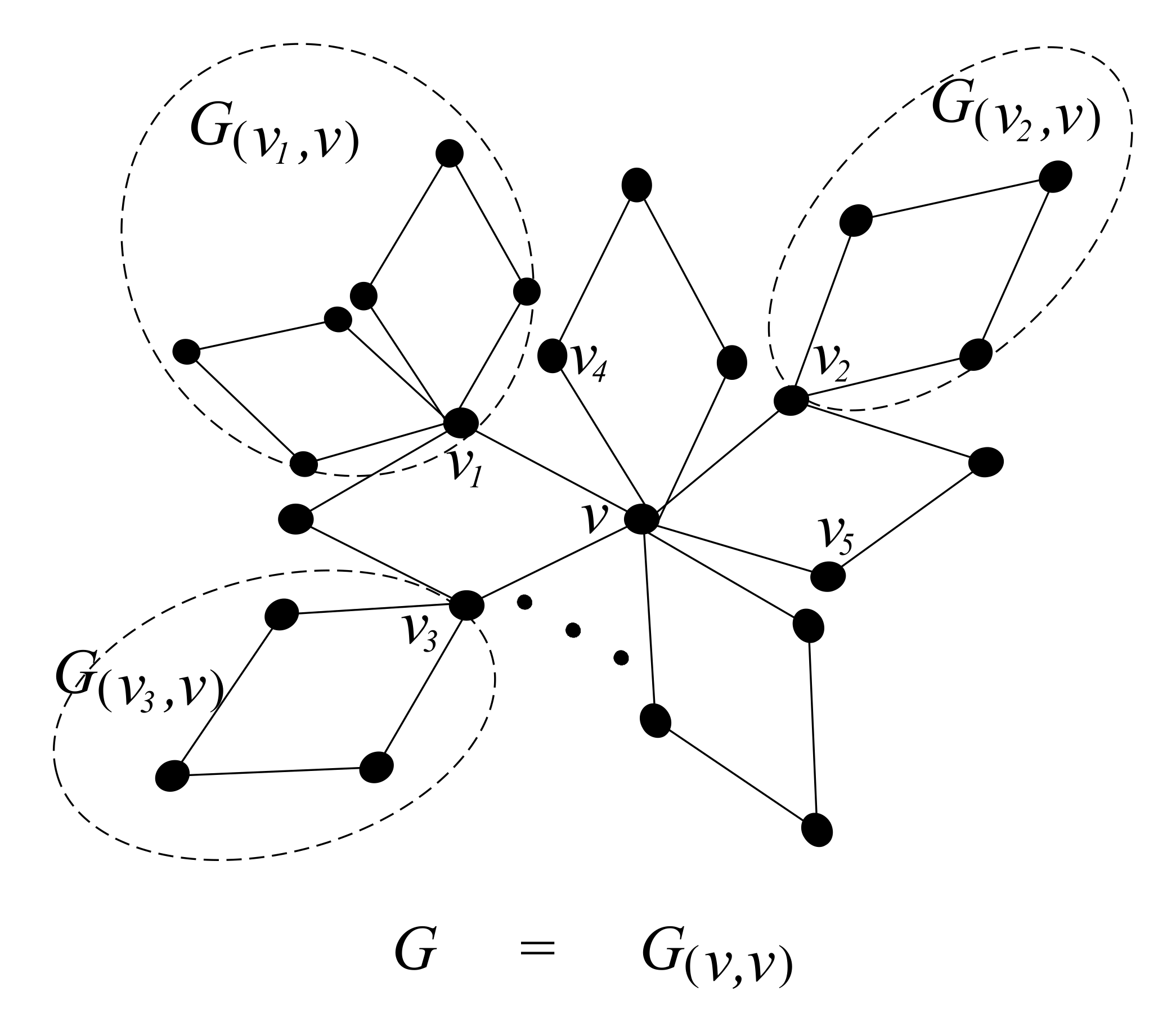
Now we study the bounds and corresponding extremal graphs over the set of block graphs having the same block order sequence. Before establishing bounds and extremal graphs, we define a notations G ( u , v ) as follows. Let ( u , v ) : u , v V ( G ) be an ordered vertex pair where u is a cut vertex of G and u v . Let G 1 be a graph obtained by removing the edges, each of which is not only incident with u but also on a simple path from u to v in G. Let G ( u , v ) be a connected component of G 1 such that G ( u , v ) contains the vertex u (see Figure 1 as an example). In particular, if u = v , then let G ( v , v ) = G .
To obtain the lower bound and the corresponding extremal graph, we define a block-slide transformation on a graph G G ( S ) in Section 4.1. A graph G which is obtained by a block-slide transformation on G satisfies both a e c c ( G ) a e c c ( G ) and G G ( S ) . For the upper bound, we define a block-shift transformation on a graph G G ( S ) in Section 4.2. A graph G which is obtained by a block-shift transformation on G satisfies both a e c c ( G ) a e c c ( G ) and G G ( S ) .

4.1. The Lower Bound and Corresponding Extremal Graphs

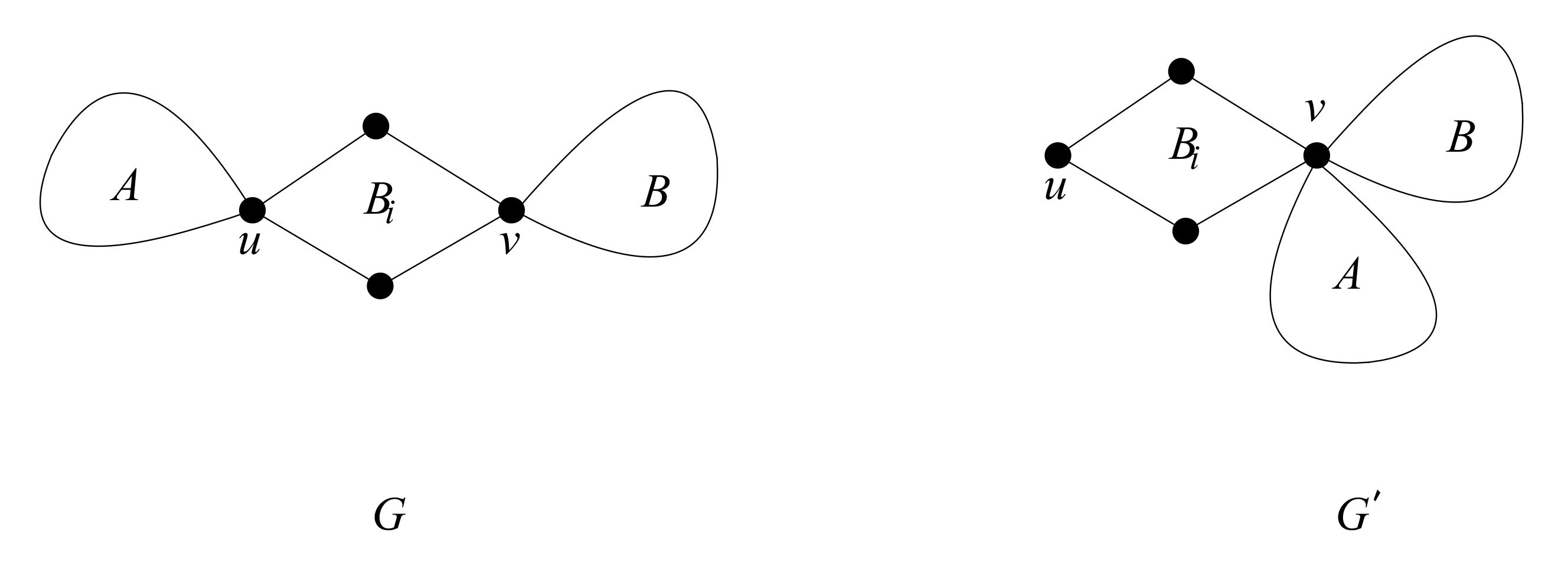
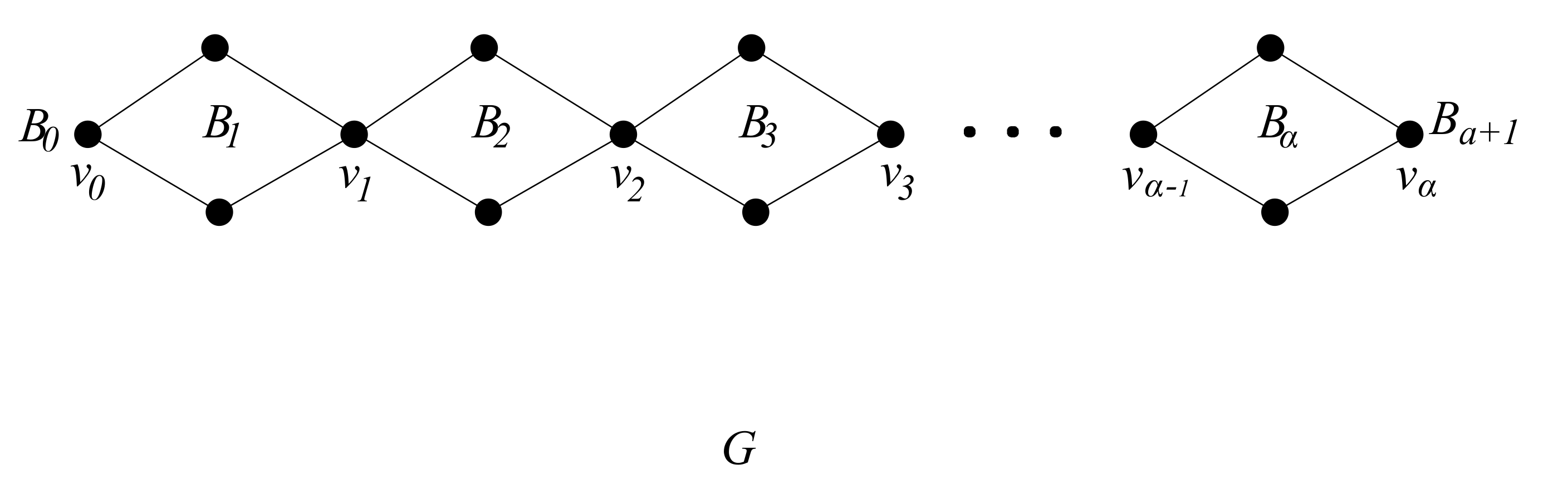
Block-slide transformation: Let B i be a block in a block graph G depicted in Figure 2, where u and v are two distinct cut-vertices of B i . Let A = G ( u , v ) and B = G ( v , u ) be two subgraphs in G (see Figure 2). Let G = G { ( u , w ) E ( G ) : w N A ( u ) } + { ( v , w ) : w N A ( u ) } . The transformation from G to G is named as a block-slide transformation on G. On the other side, the transformation from G to G is named as an inverse block-slide transformation on G , i.e., G = G { ( v , w ) E ( G ) : w N A ( v ) } + { ( u , w ) : w N A ( v ) } .
Theorem 6. 
Each block-slide transformation eliminates exactly one cut-vertex from a block graph.
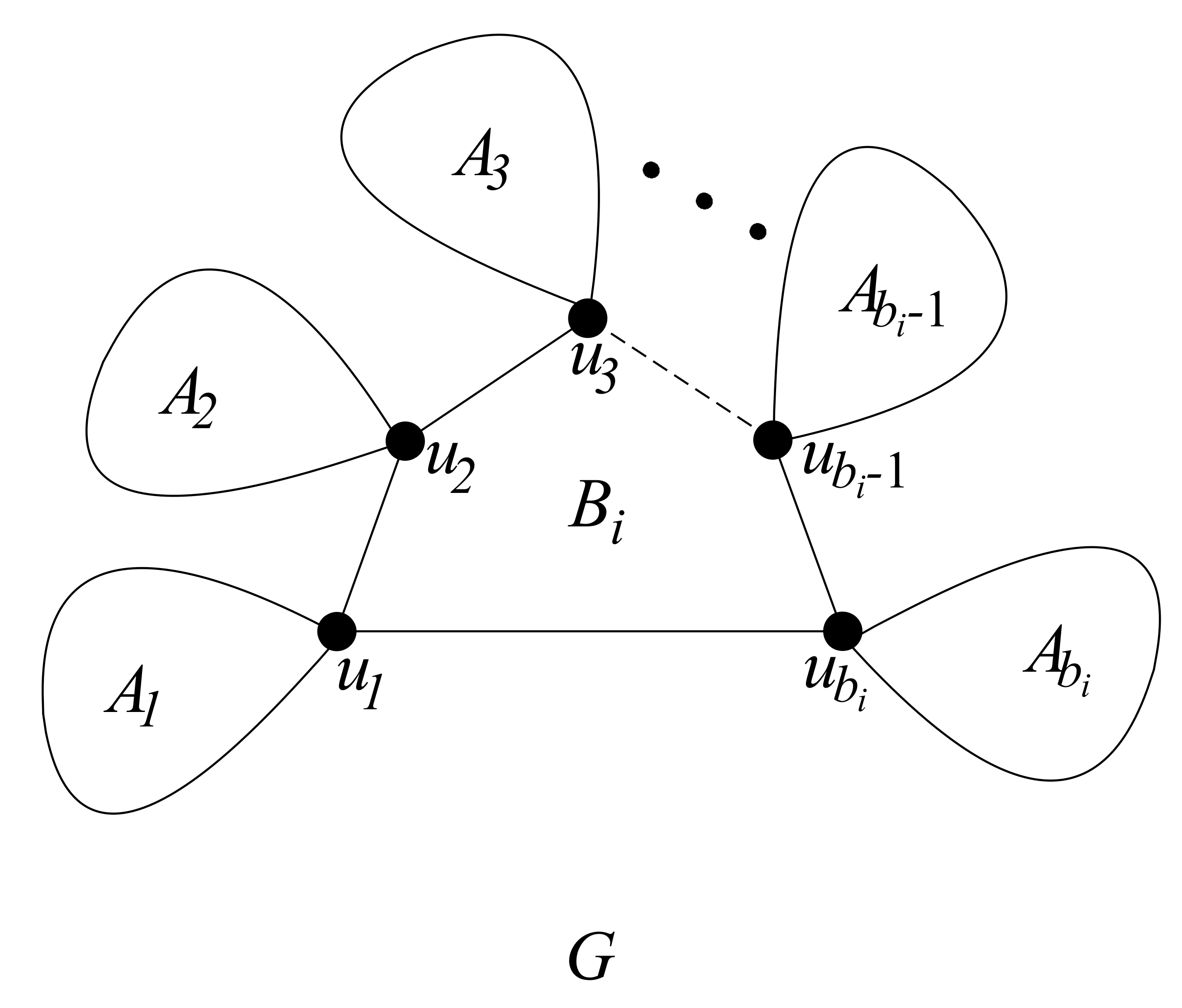
Theorem 7. 
Let G be a block graph which is obtained by a block-slide transformation on a block graph G (see Figure 2). Then a e c c ( G ) a e c c ( G ) holds.
Proof. 
Let B i be a block with order b i in G. Put the vertices of B i on a cycle and label its vertices clockwise as u = u 1 , u 2 , u 3 ,…, u b i 1 , u b i (see Figure 3). Without loss of generality, let u d i = v . There are b i + 1 parts in the graph G. They are B i , A 1 , A 2 ,…, A b i 1 , and A b i , where A 1 = A , A b i = B , and each A j is the subgraph G ( u j , u 1 ) for 2 j b i 1 . Let L = max { ϵ ( u j , A j ) : 1 j b i } . There are mainly cases of the relationship over ϵ ( u 1 , A 1 ) , ϵ ( u b i , A b i ) , and L. For each case, we consider the behavior of the average eccentricity on G in the following.
Case 1: ϵ ( u 1 , A 1 ) ϵ ( u b i , A b i ) L . For every vertex v ( 2 j b i 1 V ( A j ) ) V ( B i ) { u b i } , we have ϵ ( v , G ) = ϵ ( v , G ) . For every vertex v V ( A 1 ) { u 1 } , ϵ ( v , G ) ϵ ( v , G ) . For every vertex v V ( A b i ) , ϵ ( v , G ) ϵ ( v , G ) . Hence, the average eccentricity of the whole graph does not increase after a block-slide transformation.
Case 2: ϵ ( u b i , A b i ) < ϵ ( u 1 , A 1 ) < L . It is easy to verify that the eccentricity of every vertex in G does not change under the transformation. So the average eccentricity of the whole graph remains the same after a block-slide transformation.
Case 3: ϵ ( u b i , A b i ) < ϵ ( u 1 , A 1 ) = L . It is easy to verify that if there is a subgraph A j : 2 j b i 1 such that ϵ ( u j , A j ) = L , then the average eccentricity of the whole graph remains the same after the transformation. Let us consider the case that there is no integer j : 2 j b i 1 such that ϵ ( u j , A j ) = L .
  • ϵ ( v , G ) = ϵ ( v , G ) holds for every vertex v V ( G ) V ( A 1 ) V ( A b i ) .
  • ϵ ( v , G ) ϵ ( v , G ) holds for every vertex v V ( A 1 ) { u 1 } .
  • ϵ ( v , G ) > ϵ ( v , G ) holds for every vertex v V ( A b i ) .
  • ϵ ( u 1 , G ) ϵ ( u 1 , G ) = 1 .
As | V ( A b i ) | > 1 holds, we have a e c c ( G ) a e c c ( G ) .
Above all, the block-slide transformation does not increase the value of average eccentricity of a block graph. Hence, the theorem holds.    □
Corollary 1. 
Let G be a block graph which is obtained by an inverse block-slide transformation on a block graph G (see Figure 2). Then a e c c ( G ) a e c c ( G ) holds.
Theorem 8. 
Every block graph G with a fixed block order sequence satisfies
a e c c ( G ) 2 1 n , α > 1 1 , α = 1 ,
where α is the number of blocks in G and calculated by Equation (1).
Proof. 
Let { ( b i , s i ) : 1 i k and i , k Z } Z + × Z + be the block order sequence of the block graph G. We repeatedly apply the block-slide transformation on G until no more such transformation can be applied. As each block-slide transformation eliminates one cut-vertex, the transformation procedure must stop at a state in which there is a unique cut-vertex in the graph. In other words, we achieve a star-like block graph when no more block-slide transformation could be applied to the graph. By Theorem 7, the whole transformation procedure does not increase the average eccentricity. Hence, an n-order star-like block graph reaches the minimum value of the average eccentricity among all block graphs with order n. Finally, by Equation (4), if there is more than one block in G, then a e c c ( G ) 2 1 n . Otherwise, the lower bound is exactly one.    □

4.2. The Upper Bound and Corresponding Extremal Graphs

In this section, we define a block-shift transformation on a block graph and then we present an upper bound on a graph under the help of such a transformation.
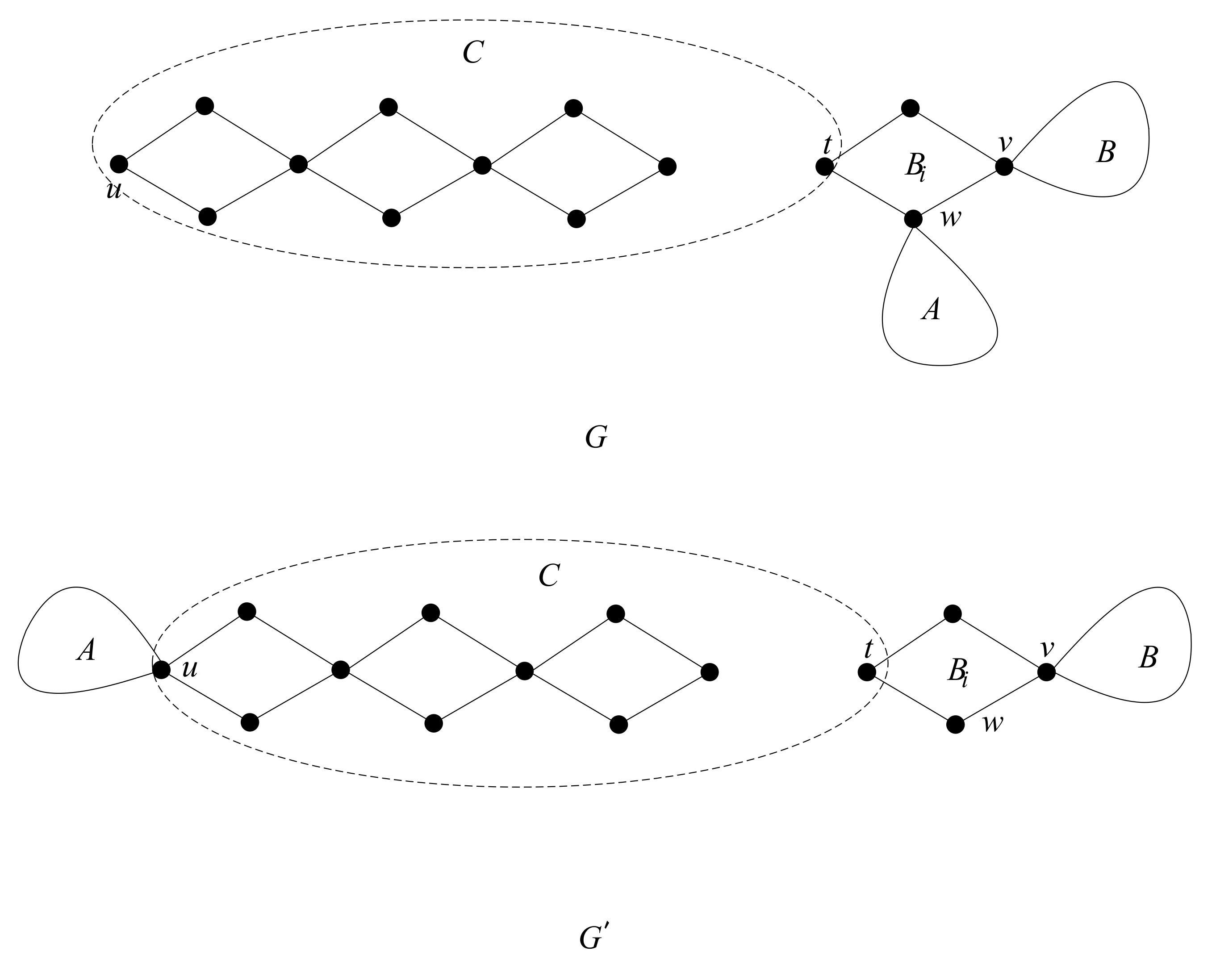
Let t be a cut-vertex of a block graph G and E ( t ) be the set of edges which are all incident with t. Let R ( t ) be a partition of E ( t ) such that two edges ( u , t ) , ( v , t ) E ( G ) belong to the same element of R ( t ) if and only if u and v are in the same block of G. For every element a R ( t ) , the petal G ( a , t ) corresponding to a is defined as follows. G ( a , t ) is a connected component of such a graph which is obtained by deleting the edges in b R ( t ) , b a b from G, and contains the cut-vertex t.
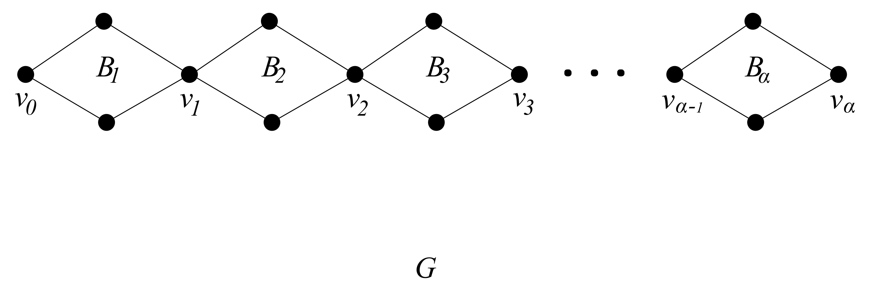
In this section, we will see a special kind of block graph which is named a path-like block graph. A block graph G is named a path-like block graph if it either is a complete graph or has exactly two pendent blocks while each of the other blocks contains exactly two cut-vertices.
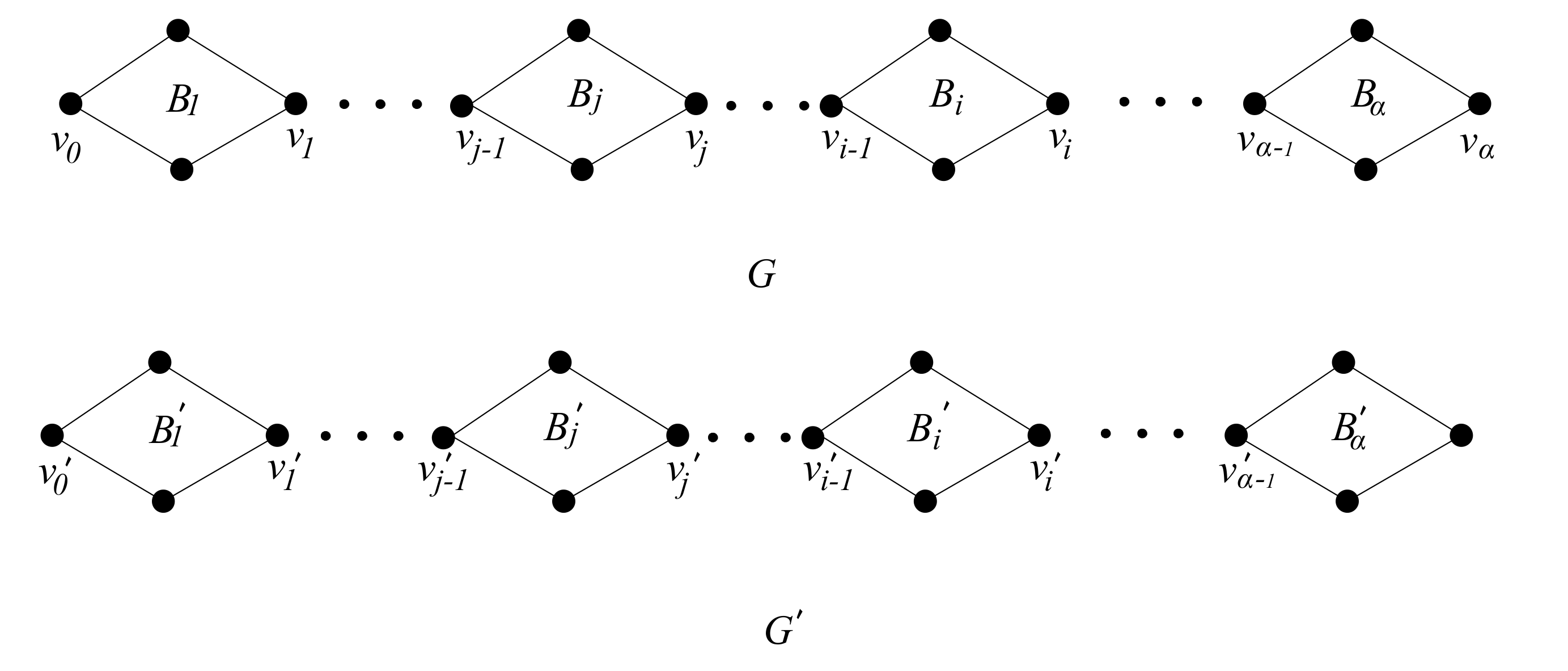
Block-shift transformation: Let B i be a block in a block graph G where t, v, and w are all cut-vertices in B i as depicted in Figure 4. Note that the three cut-vertices t, w, and v do not need to be distinct to each other. Let C be a petal at the vertex t such that C is a path-like block graph and does not contain the block B i . Let u V ( C ) be a pendent vertex of G. Let A and B be two sets of petals corresponding, respectively, to vertices w and v, such that ϵ ( w , A ) ϵ ( v , B ) holds. Let G = G { ( w , s ) E ( G ) : s N A ( w ) } + { ( u , s ) : s N A ( w ) } . Then the transformation from G to G is said to be a block-shift transformation on graph G, while the transformation from G to G is said to be an inverse block-shift transformation on graph G , i.e., G = G { ( u , s ) E ( G ) : s N A ( u ) } + { ( w , s ) : s N A ( u ) } .
Theorem 9. 
Let G be a block graph which is obtained by a block-shift transformation on a block graph G (see Figure 4). Then a e c c ( G ) a e c c ( G ) holds.
Proof. 
It is obvious that the eccentricity of every vertex in A and B does not decrease under the block-shift transformation. As ϵ ( w , A ) ϵ ( v , B ) , the eccentricity of every vertex in the set V ( C ) V ( B i ) also could not be decreased by the block-shift transformation. Above all, after a block-shift transformation, the average eccentricity of a block graph does not decrease.    □
Corollary 2. 
Let G be a block graph which is obtained by an inverse block-shift transformation on a block graph G (see Figure 4). Then a e c c ( G ) a e c c ( G ) holds.
Repeatedly apply the block-shift transformation on a block graph G. Finally we will reach a state that the graph G turns into a path-like block graph. By Theorem 9, the transformation does not decrease the average eccentricity, so the upper bound on block graph set G ( S ) must be achieved by a path-like block graph in G ( S ) . Let P G m a x S be a path-like block graph with the maximum average eccentricity among all path-like block graphs in G ( S ) . The upper bound on the set G ( S ) can be written in the following Theorem 10.
Theorem 10. 
Let G G ( S ) be a block graph with the set S as its block order sequence. Then,
a e c c ( G ) a e c c ( P G m a x S )
The following Section 5 is to present a method to obtain a P G m a x S .

5. Bounds and Extremal Graphs for Path-like Block Graphs

This section settles bounds and extremal graphs for path-like block graphs. Initially, formulas are established to calculate the average eccentricity on a path-like block graph. Then, we set up bounds and their corresponding extremal graphs for the set of path-like block graphs, where every path-like block graph has the same block order sequence S. Finally, we prove lower and upper bounds on the set of path-like block graphs, where each path-like block graph has order n.

5.1. Formulas for the Average Eccentricity on Path-like Block Graphs with Given Block Order Sequence

Let PG ( S ) G ( S ) be the set of path-like block graphs with the block order sequence S Z + × Z + . For a path-like block graph G PG ( S ) , we straighten G on a horizontal line from left to right as in Figure 5. Then, we label the blocks as B 1 , B 2 , B 3 ,…, B α and label the cut-vertices as v 1 , v 2 , v 3 ,…, v α 1 in G from left to right, one by one, where α is the number of blocks in G as calculated by Equation (1) in Theorem 1. In particular, we choose a non-cut-vertex from B 1 and a non-cut-vertex from B α , and then label them v 0 and v α , respectively. In the following, every path-like block graph has already been straightened and labeled this way. In order to make it clear, in the following, we use N i ( 1 i α ) to stand for the order of each block B i , i.e., N i = | V ( B i ) | . Let β = Σ i = 1 α / 2 ( N i + N α i + 1 ) ( α i + 1 ) .
Theorem 11. 
Let G PG ( S ) where S Z + × Z + is a block order sequence. Then, the average eccentricity of G is,
  • If the number of blocks α is even, then
    a e c c ( G ) = 1 n ( β 3 4 α 2 )
  • If the number of blocks α is odd, then
    a e c c ( G ) = 1 n ( β α + 1 2 N ( α + 1 ) / 2 3 4 ( α 2 1 ) )
    where n and α are the order and the number of blocks in G as calculated in Equations (2) and (1), respectively.
Proof. 
If α is even, then in block B i and B α i + 1 for every 1 i α 2 , there are exactly N i + N α i + 1 2 vertices, each of which contributes the value α i + 1 to the average eccentricity. The middle cut vertex v α / 2 exactly contributes the value α 2 . To sum all, the average eccentricity of G is
a e c c ( G ) = 1 n ( Σ i = 1 α / 2 ( N i + N α i + 1 2 ) ( α i + 1 ) + α 2 ) = 1 n ( Σ i = 1 α / 2 ( N i + N α i + 1 ) ( α i + 1 ) 2 Σ i = 1 α / 2 ( α i + 1 ) + α 2 ) = 1 n ( β 3 4 α 2 )
If α is odd, then in block B i and B α i + 1 for every 1 i α 2 = α 1 2 , there are exactly N i + N α i + 1 2 vertices, each of which contributes the value α i + 1 to the average eccentricity. In addition, each vertex in the middle block B ( α / 2 ) contributes the value n 2 = n + 1 2 . To sum all, the average eccentricity of G is
a e c c ( G ) = 1 n ( Σ i = 1 ( α 1 ) / 2 ( N i + N α i + 1 2 ) ( α i + 1 ) + α + 1 2 N α / 2 ) = 1 n ( Σ i = 1 α / 2 ( N i + N α i + 1 2 ) ( α i + 1 ) α + 1 2 ( N α / 2 2 ) ) = 1 n ( Σ i = 1 α / 2 ( N i + N α i + 1 ) ( α i + 1 ) 2 Σ i = 1 α / 2 ( α i + 1 ) α + 1 2 N α / 2 + ( α + 1 ) ) = 1 n ( β α + 1 2 N ( α + 1 ) / 2 3 4 ( α 2 1 ) )
   □

5.2. Extremal Graphs for Path-like Block Graphs with Given Block Order Sequence

In order to set up bounds and study extremal graphs for path-like block graphs, we need to establish a graph transformation operation which is named as block-exchange transformation. To make the transformation clear, we define a mapping function M ( i ) to map the subscript index i of B i ( 1 i α ) into a new integer as follows.
  • If α is even, then
    M ( i ) = i 1 i α 2 α 2 i = α 2 + 1 M ( i 1 ) 1 α 2 + 2 i α
  • If α is odd, then
    M ( i ) = i 1 i α 2 M ( i 1 ) 1 α 2 + 1 i α
Lemma 2. 
For every block B i ( 1 i α ) in a path-like block graph G, there are exactly N i 1 vertices, each of which has the eccentricity equal to α M ( i ) + 1 .
Proof. 
We prove this lemma by considering the case that α is even. It is the same way to give proof for the case that α is odd. There are three cases.
Case 1: 1 i α 2 . The eccentricity of every vertex u V ( B i ) { v i } is α i + 1 = α M ( i ) + 1 , while the vertex v i has its eccentricity equal to the value of α i . Hence, the lemma holds on this case.
Case 2: i = α 2 + 1 . The eccentricity of every vertex u V ( B i ) { v i 1 } is equal to α 2 + 1 = α α 2 + 1 = α M ( i ) + 1 , while the vertex v i 1 has the eccentricity as α 2 . Hence, the lemma holds on this case.
Case 3: α 2 + 2 i α . The eccentricity of every vertex u V ( B i ) { v i 1 } is α M ( i ) + 1 , while the vertex v i 1 has the value of α M ( i ) . Hence, the lemma holds on this case.
Above all, there are exactly N i 1 vertices each of which has the eccentricity equal to α M ( i ) + 1 for every block B i ( 1 i α ) in a path-like block graph G.    □
Block-exchange transformation: Let G be a path-like block graph with labeled blocks and cut-vertices as depicted in Figure 5. If there are two distinct blocks B i , B j ( 1 i , j α ) such that both N i < N j and M ( i ) < M ( j ) hold, then we construct a new graph G by exchanging the two blocks B i and B j in G, i.e., G = G { ( v i 1 , u ) : u N B i ( v i 1 ) } { ( v i , u ) : u N B i ( v i ) } + { ( v j 1 , u ) : u N B i ( v i 1 ) } + { ( v j , u ) : u N B i ( v i ) } { ( v j 1 , u ) : u N B j ( v j 1 ) } { ( v j , u ) : u N B j ( v j ) } + { ( v i 1 , u ) : u N B j ( v j 1 ) } + { ( v i , u ) : u N B j ( v j ) } (see Figure 6). The transformation from G to G is called a block-exchange transformation on G. On the other side, the transformation from G to G is said to be an inverse block-exchange transformation on G . Note that, after the block-exchange transformation, B i B j and B j B i holds in graph G .
Theorem 12. 
Let G be a path-like block graph which is obtained by a block-exchange transformation on a block graph G (see Figure 6). Then a e c c ( G ) > a e c c ( G ) holds.
Proof. 
Let B i and B j be two blocks such that both N i < N j and M ( i ) < M ( j ) hold in a path-like block graph G. Let G be the new graph obtained by a block-exchange transformation on these two blocks. By the definition of the eccentricity, the eccentricity of every vertex in V ( G ) V ( B i ) V ( B j ) { v i 1 , v i , v j 1 , v j } does not change under the block-exchange transformation. As M ( i ) < M ( j ) , by Lemma 2, the eccentricity of each vertex in V ( B i ) { v i 1 , v i } decreases ( α M ( i ) + 1 ) ( α M ( j ) + 1 ) = M ( j ) M ( i ) , while the eccentricity of each vertex in V ( B j ) { v j 1 , v j } increase ( α M ( i ) + 1 ) ( α M ( j ) + 1 ) = M ( j ) M ( i ) after the block-exchange transformation. On the whole, relying on Equations (5) and (6), the change of the average eccentricity under such a transformation is
a e c c ( G ) a e c c ( G ) = 1 n ( ( ( N i 1 ) ( α M ( i ) + 1 ) + ( N j 1 ) ( α M ( j ) + 1 ) ) ( ( N j 1 ) ( α M ( i ) + 1 ) + ( N i 1 ) ( α M ( j ) + 1 ) ) ) = 1 n ( N i N j ) ( M ( j ) M ( i ) )
As M ( i ) < M ( j ) and N i < N j hold, ( N i N j ) ( M ( j ) M ( i ) < 0 must hold. Therefore, the block-exchange transformation increases the average eccentricity of a path-like block graph.    □
Corollary 3. 
Let G be a path-like block graph which is obtained by an inverse block-exchange transformation on a block graph G (see Figure 6). Then a e c c ( G ) > a e c c ( G ) holds.
Let P G m i n S and P G m a x S be path-like block graphs having, respectively, minimum and maximum average eccentricity on the set of block graphs with block order sequence S. In other words, let P G m i n S PG ( S ) G ( S ) be a path-like block graph with the block order sequence S where every two distinct blocks B i and B j of P G m i n S satisfies that both N i < N j and M ( i ) < M ( j ) hold. Let P G m a x S PG ( S ) be a path-like block graph with the block order sequence S where every two distinct blocks B i and B j of P G m a x S satisfies that both N i < N j and M ( i ) > M ( j ) hold.
Theorem 13. 
The average eccentricity of every graph G PG ( S ) with block order sequence S is not less than that of P G m i n S and not larger than that of P G m a x S , i.e.,
a e c c ( P G m i n S ) a e c c ( G ) a e c c ( P G m a x S )
Proof. 
Repeatedly applying the block-exchange transformation on graph G until there is no pair of blocks B i and B j such that both N i < N j and M ( i ) < M ( j ) hold, we obtain a graph P G m a x S PG ( S ) . By Theorem 12, every block-exchange transformation on graph G increases the average eccentricity. Hence, a e c c ( G ) a e c c ( P G m a x S ) holds.
Repeatedly applying the inverse block-exchange transformation on graph G until there is no pair of blocks B i and B j such that both N i < N j and M ( i ) > M ( j ) hold, we obtain a graph P G m i n S PG ( S ) . By Corollary 3, every block-exchange transformation on graph G increases the average eccentricity. Hence, a e c c ( P G m i n S ) a e c c ( G ) holds.    □

5.3. Bounds on Path-like Graphs with Order n

Theorem 14. 
Let G be a path-like block graph with the order n. Then we have
1 a e c c ( G ) 1 n 3 4 n 2 1 2 n
Proof. 
We straighten the graph G relying on the method stated in Section 5.1. The blocks are labeled B 1 , B 2 , B 3 ,…, B α and the cut-vertices are labeled v 1 , v 2 , v 3 ,…, v α 1 in G from left to right, one by one, where α is the number of blocks in G as calculated by Equation (1) in Theorem 1. We regard each non-cut-vertex of B 1 and B α as an empty block graph, where an empty block graph is a graph having exactly one vertex. Then, we pick just one non-cut-vertex of B 1 and label it B 0 , while one non-cut-vertex of B n α is labeled B α + 1 , see Figure 7.
Considering the additional labels B 0 and B α + 1 , we slightly modify the mapping function M ( i ) as follows, where M ( i ) is the mapping function defined in Equations (7) and (8). A new mapping function M ( i ) , which maps the subscript index i of B i : 0 i α + 1 into a new integer, is defined in the following Equation (9).   
M ( i ) = 0 i = 1 o r i = α + 1 M ( i ) 1 i α
In the following proof, we still use N i to stand for the order of block B I for every 0 i α + 1 . If there is a non-cut vertex v V ( B i ) and a block B j such that 1 i α , 0 j α + 1 , N i 3 , and M ( i ) > M ( j ) , then let G = G { ( v , u ) : u N B i ( v ) } + { ( v , u ) : u V ( B j ) } . Repeatedly apply this vertex-moving operation on the vertices of G until no more such operation can be achieved. Then we obtain a path P n . Recall that every such vertex-moving operation increases the average eccentricity. Therefore, the average eccentricity of G could not exceed that of a path P n . Recall that the average eccentricity of an n-order path P n is 1 n 3 4 n 2 1 2 n [4].
On the other hand, if there is a non-cut-vertex v V ( B i ) and a block B j such that 0 i α + 1 , 1 j α , N i < n , and M ( i ) < M ( j ) , then let G = G { ( v , u ) : u N B i ( v ) } + { ( v , u ) : u V ( B j ) } . Repeatedly apply this vertex-moving operation on the vertices of G until no more such operation can be achieved. We will subsequently obtain either a block graph with only one block or a block graph with exactly two blocks. If the final graph has only one block, then it is a complete graph K n . Recall that every such vertex-moving operation decrease the average eccentricity. If the final graph has exactly two blocks, say B 1 and B 2 , then we delete all edges in B 2 and add an edge between each vertex v V ( B 1 ) and u V ( B 2 ) . Then we still obtain a complete graph K n , and this process decreases the average eccentricity. It is easy to verify that the average eccentricity of a complete graph K n is exactly one [4].
Above all, we have 1 a e c c ( G ) 1 n 3 4 n 2 1 2 n , where G is a path-like block graphs with order n.    □

6. Extracting the Block Order Sequence of a Block Graph

In this section, we devised a linear time algorithm to extract the block order sequence of a block graph. This indicates that it is possible to study the eccentricity on block graphs via its block order sequence.

6.1. To Decide a Cut-Vertex

Our algorithm needs to test whether a vertex is a cut-vertex The idea benefits from a property of cut-vertices in a block graph, which is stated in Lemma 3 and realized by Algorithm 2. We should emphasize that Lemma 3 is fit for the block graphs rather than the general undirected simple graphs.
Lemma 3. 
Let G be a block graph and v V ( G ) . Let u be a neighbor of v in G. Then u is a cut-vertex of G if and only if there is a vertex w N G ( u ) such that ( v , w ) E ( G ) .
Proof. 
Let G be the graph obtained by deleting vertex u from G. We prove this lemma from the following two sides.
On the one hand, if there is a vertex w N G ( u ) such that ( v , w ) E ( G ) , then v and w is also not adjacent in G . We claim that w and v are disconnected in G . Otherwise, both in graph G and G , there must be a path P from v to w such that u V ( P ) . The path P = v u w is another path from w to v in G and is vertex-internally-disjointed with the path P. Hence, there is a cycle in G which contains the three vertices u, v, and w, so the three vertices u, v, and w are all in the same block of G. As G is a block graph, every block is a clique, so there is an edge incident with both v and w, which comes to a contradiction. Hence, u must be a cut-vertex of G.
On the other hand, if u is a cut-vertex of G, then G must be a disconnected graph. Recall that the graph G is connected. Moreover, there must be two distinct vertices a V ( G ) and b V ( G ) such that every simple path from a to b in G must go through the vertex u [19], as u is a cut-vertex. Let P 1 be an arbitrary simple path from a to b in G. Without loss of generality, let w 1 V ( P 1 ) and w 2 V ( P 1 ) satisfy ( w 1 , u ) E ( P 1 ) and ( w 2 , u ) E ( P 1 ) , and the sub-path a w 1 of P 1 from a to w 1 do not contain the vertex u. Then the path P 1 can be marked as a w 1 u w 2 b . Assume that every vertex t N G ( u ) { v } is adjacent to v in the graph G. Then the path P 1 = a w 1 v w 2 b is another path from a to b. Then P 1 is another simple path, while not containing u at all. This comes to a contradiction.
Above all, the vertex u is a cut-vertex of G if and only if there is a neighbor w N G ( u ) of u such that ( v , w ) E ( G ) .    □
By Lemma 3, it is exciting to find that, in order to decide whether u is a cut-vertex of a block graph G, one just needs to access all edges which are incident with u rather than decide the connectivity of G. It would therefore take far less time to decide whether a vertex is a cut-vertex in a block graph by use of the property stated in Lemma 3. We realize this decision method in the following Algorithm 2.
Theorem 15. 
Given a vertex v of a graph G and a neighbor u N G ( v ) of v, it spends O ( | N G ( u ) | ) time to decide whether u is a cut-vertex by Algorithm 2.
Proof. 
In step 2–2 of Algorithm 2, each neighbor of u is either adjacent to v or not adjacent to v. Moreover, every neighbor of u is visited once and only once. Hence, the time complexity is O ( | N G ( u ) | ) .    □

6.2. To Obtain a Block Order Sequence

To find the block order sequence of a block graph G we must first to find every block and then calculate the order for each block, which is realized in Algorithm 1.
Lemma 4. 
Let u be a non-cut-vertex in a block B i of a block graph G, then the order of B i is equal to | N G ( u ) | + 1 .
Proof. 
As u is not a cut-vertex, u and all its neighbors N G ( u ) must be in the same block B i . As every block in a block graph must be a clique, there is no vertex w V ( B i ) such that ( u , w ) E ( G ) . Therefore, the vertex set V ( B i ) is equal to { u } N G ( u ) . Hence, the order of B i is | N G ( u ) | + 1 .    □
Now let us turn to Algorithm 1. The algorithm is to find the block order sequence of a block graph by means of searching the cut-vertices one by one, as every block must associate with some cut-vertex. The whole Algorithm is a recursive depth-first search (DFS) procedure [2] beginning with an arbitrary vertex of a block graph. The process to search for the cut-vertices is an “up-to-bottom” recursive method. The process to calculate the order for each block is performed the back-trace way during the recursive process from bottom to up.
By Lemma 1, the algorithm can always meet with a pendent block, say B i , at the bottom of a recursive process. Let w be the unique cut-vertex in B i . By Lemma 4, the algorithm calculate the order of B i by means of { w } N G ( w ) where w V ( B i ) is not a cut-vertex and adjacent to w. After all the pendents block corresponding to w has been processed, the algorithm marks w as an non-cut-vertex by step 1. Then, the algorithm traces back to search another block. By this way going up, finally, we can obtain a block order sequence of a block graph.
Algorithm 1: Seq(G, v, visit, B)
Axioms 11 00114 i001
Algorithm 2: Is_CutVertex(G, v, u)
Axioms 11 00114 i002
Theorem 16. 
It takes O ( n + m ) time for the Algorithm 1 to find the block order sequence of a block graph G where n and m are the order and the size of G, respectively.
Proof. 
Without loss of generality, let Algorithm 1 execute beginning with the vertex v. Let T ( w , G ( w , v ) ) be the time taken by Algorithm 1 on the subgraph G ( w , v ) . Let C be the set of cut-vertices in G. Then we have,
T ( v , G ( v , v ) ) = Σ u N G 1 ( v ) ( O ( | N G ( u ) | ) + T ( u , G ( u , v ) ) ) + Σ u N G ( v ) ( O ( | N G ( u ) | ) + O ( 1 ) ) = Σ u C ( O ( | N G ( u ) | ) ) + Σ u V ( G ) ( O ( | N G ( u ) | ) ) + O ( n ) 2 Σ u V ( G ) ( O ( | N G ( u ) | ) + O ( n ) = O ( n + m )

7. Conclusions

We study the average eccentricity of block graphs from the perspective of their block order sequences. A block order sequence could provide useful structural information on block graphs and can be obtained in linear time from Algorithm 1. Moreover, via Theorem 3, the perspective of block order sequences naturally provides an equivalence relationship on the set of block graphs. It may be interesting to study some other computational problems and mathematical properties on block graphs from the perspective of block order sequences. Recall that the blocks in the other graph classes may not be all cliques. Moreover, an entire graph can be characterized by applying several criteria [21,22]. In particular, in chemical graph theory, several connections between graph structure and properties have been established [23]. This paper characterizes a block graph from block order sequence. Are there any ways to deal with problems on the other graph classes, also from the perspective of block order sequence?

Author Contributions

Conceptualization, X.L. and G.Y.; Methodology, X.L. and G.Y.; Writing-Original Draft Preparation, X.L.; Writing-Review and Editing, G.Y. and K.C.D. Supervision, G.Y. and K.C.D.; Validation, X.L., G.Y. and K.C.D. All authors have read and agreed to the published version of the manuscript.

Funding

This work was supported by Science Foundation of Guizhou University of Finance and Economics (2020XYB16), Science Foundation of Guizhou University of Finance and Economics (2019YJ058).

Institutional Review Board Statement

Not applicable.

Informed Consent Statement

Not applicable.

Data Availability Statement

Not applicable.

Conflicts of Interest

The authors declare no conflict of interest.

References

  1. Buckley, F.; Harary, F. Distance in Graphs; Addisson-Wesley: Redwood City, CA, USA, 1990. [Google Scholar]
  2. Cormen, T.H.; Leiserson, C.E.; Rivest, R.L.; Stein, C. Introduction to Algorithme; MIT Press: Cambridge, UK, 2001. [Google Scholar]
  3. Ali, P.; Dankelmann, P.; Morgan, M.J.; Mukwembi, S.; Vetrik, T. The average eccentricity, spanning trees of plane graphs, size and order. Util. Math. 2018, 107, 37–49. [Google Scholar]
  4. Dankelmann, P.; Goddard, W.; Swart, C.S. The average eccentricity of a graph and its subgraphs. Util. Math. 2004, 41, 41–51. [Google Scholar]
  5. Dankelmann, P.; Mukwembi, S. Upper bounds on the average eccentricity. Discret. Appl. Math. 2014, 167, 72–79. [Google Scholar] [CrossRef]
  6. Dankelmann, P.; Osaye, F.J. Average eccentricity, k-packing and k-domination in graphs. Discret. Math. 2019, 342, 1261–1274. [Google Scholar] [CrossRef]
  7. Dankelmann, P.; Osaye, F.J.; Mukwembi, S.; Rodrigues, B. Upper Bounds on the average eccentricity of K3-free and C4-free graphs. Discret. Appl. Math. 2019; in press. [Google Scholar] [CrossRef]
  8. Du, Z.; Ilić, A. On AGX conjectures regarding average eccentricity. MATCH Commun. Math. Comput. Chem. 2013, 69, 597–609. [Google Scholar]
  9. Du, Z.; Ilić, A. A proof of the conjecture regarding the sum of the domination number and average eccentricity. Discret. Appl. Math. 2016, 201, 105–113. [Google Scholar] [CrossRef]
  10. Ilić, A. On the extremal properties of the average eccentricity. Comput. Math. Appl. 2012, 64, 2877–2885. [Google Scholar] [CrossRef] [Green Version]
  11. Smith, H.; Székely, L.A.; Wang, H. Eccentricity sum in trees. Discret. Appl. Math. 2016, 207, 120–131. [Google Scholar] [CrossRef] [Green Version]
  12. Tang, Y.; Zhou, B. On average eccentricity. MATCH Commun. Math. Comput. Chem. 2012, 67, 405–423. [Google Scholar]
  13. Ghorbani, M.; Li, X.; Maimani, H.R.; Mao, Y.; Rahmani, S.; Rajabi-Parsa, M. Steiner (revised) Szeged index of graphs. MATCH Commun. Math. Comput. Chem. 2019, 82, 733–742. [Google Scholar]
  14. Lei, H.; Shi, Y.; Yue, J. A Survey on the Wiener Polarity Index. MATCH Commun. Math. Comput. Chem. 2021, 86, 289–318. [Google Scholar]
  15. Yu, G.; Feng, L. On the connective eccentricity index of graphs. MATCH Commun. Math. Comput. Chem. 2013, 69, 611–628. [Google Scholar]
  16. Zhou, B.; Du, Z. On eccentric connectivity index. MATCH Commun. Math. Comput. Chem. 2010, 63, 181–198. [Google Scholar]
  17. Mao, Y.; Furtulab, B. Steiner Distance in Chemical Graph Theory. MATCH Commun. Math. Comput. Chem. 2021, 86, 211–287. [Google Scholar]
  18. Zaheer Ahmad, A.Q.; Baig, M.; Azhar, M. Imran Total eccentricity and average eccentricity indices of some chemical graphs: Carbon graphite and copper oxide. J. Inf. Optim. Sci. 2020, 41, 905–924. [Google Scholar]
  19. Bondy, J.A.; Murty, U.S.R. Graph theory with applications. In Great Britain; The Macmillan Press: Stuttgart, Germany, 1976. [Google Scholar]
  20. Goddard, W.; Rosen, K.H.; Shier, D.R. Handbook of Discrete and Combinatorial Mathematics, 2nd ed.; Chapman and Hall: London, UK; CRC Press: Boca Raton, FL, USA, 2018. [Google Scholar]
  21. Jäntschi, L.; Diudea, M. Subgraphs of pair vertices. J. Math. Chem. 2019, 45, 364–371. [Google Scholar] [CrossRef]
  22. Jäntschi, L.; Balan, M.C.; Bolboacă, S. Counting Polynomials on Regular Iterative Structures. Appl. Med. Inform. 2009, 24, 67–95. [Google Scholar]
  23. Diudea, M.V.; Gutman, I.; Jantschi, L. Molecular Topology; Nova Science Publishers: New York, NY, USA, 2001. [Google Scholar]
Figure 1. The kinds of neighbors of v and the subgraphs G ( v i , v ) : i = 1 , 2 , 3 in a block graph G.
Axioms 11 00114 g001
Figure 2. G is obtained by a block-slide transformation from G, where u and v are on the same block B i and are two distinct cut-vertices of B i .
Axioms 11 00114 g002
Figure 3. The configuration of a block graph G, when we focus on the block B i .
Axioms 11 00114 g003
Figure 4. G is obtained by a block-shift transformation from G where v, t, and w are all cut-vertices on the same block B i . Note that the three cut-vertices v, t, and w are not restricted to be distinct. The longest path which ends with w in the subgraph A is not longer than the longest path which ends with v in the subgraph B. Moreover, the subgraph C is a path-like block subgraph.
Axioms 11 00114 g004
Figure 5. A path-like block graph G is straightened on a horizontal line from left to right and labeled B 1 , B 2 , B 3 ,…, B α one by one, where α is the number of blocks in G.
Axioms 11 00114 g005
Figure 6. G is obtained by a block-exchange transformation from G, where B i B j , B j B i , and B s B s for s i , s j . Moreover, v s = v s for every 1 s α 1 .
Axioms 11 00114 g006
Figure 7. A path-like block graph G is straightened on a horizontal line from left to right and labeled B 1 , B 2 , B 3 ,…, B α one by one, where α is the number of blocks in G, where the two non-cut-vertices v 0 and v α are labeled B 0 and B α + 1 , respectively.
Axioms 11 00114 g007
Publisher’s Note: MDPI stays neutral with regard to jurisdictional claims in published maps and institutional affiliations.

