Article

Analyzing the Causality and Dependence between Exchange Rate and Real Estate Prices in Boom-and-Bust Markets: Quantile Causality and DCC Copula GARCH Approaches

1
Center of Excellence in Econometrics, Faculty of Economics, Chiang Mai University, Chiang Mai 50200, Thailand
2
Faculty of Economics, Shandong University of Finance and Economics, Jinan 250000, China
3
Faculty of Economics, Chiang Mai University, Chiang Mai 50200, Thailand
4
Department of Mathematics, Kent State University, Warren, OH 44483, USA
*
Author to whom correspondence should be addressed.
Axioms 2022, 11(3), 113; https://doi.org/10.3390/axioms11030113
Submission received: 1 February 2022 / Revised: 23 February 2022 / Accepted: 28 February 2022 / Published: 3 March 2022
(This article belongs to the Section Mathematical Analysis)

Abstract

:
Unlike most previous studies examining the causal relationship and dependence between exchange rates and real estate prices, this study aims to investigate the causal relationship and dependence between these two variables in a boom-and-bust market setting using the panel quantile Granger causality and dynamic conditional correlation (DCC) copula GARCH approaches, respectively. In the panel quantile Granger causality test, quantiles 0.1 and 0.9 are considered to represent extreme markets (bust and boom, respectively). Our first results showed the causal effects at extreme quantiles to be very different from those at the median quantile. We also found a greater causality between house prices and exchange rates in the boom market compared to the bust market. In the second model, we explored the relationship between exchange rates and real estate prices, taking boom-and-bust dynamics into account by measuring the tail dependence through the DCC copula GARCH method. Our findings confirm the strong time-varying tail dependence between house prices and exchange rates. The degree of tail dependence was quite stable over the sample period, except for the periods around 1997–1998 and 2008–2009, when the degree of tail dependence was stronger and less persistent. These two periods correspond to the two great financial crises in Asia and the USA, respectively.

1. Introduction

The need for food and shelter is primordial among humans and other creatures. House prices are not only closely related to the cost of living but also reflect the states of entire economies. Real estate is an established market that plays a vital role in economic development and is a key factor affecting national economies and people’s livelihood; buying a used building is generally viewed as final product consumption while buying a new building is an investment in GDP [1]. Since the beginning of the 21st century, real estate prices around the world have continued to rise, and different levels of “prosperity” have emerged in developed and developing countries [2]. Moreover, the real estate market has attracted the attention of domestic and foreign investors to a large extent, and the demand for investment or speculation is quite high nowadays [3]. Changes in housing prices in the real estate market are particularly prominent in economically developed countries and regions. In some economically prosperous cities and countries, housing prices are rising very rapidly. Some economists regard housing prices as an indicator of economic development [4,5].
As housing is a necessity, housing prices are always a very popular topic for discussion and many people are keen to predict trends. Meanwhile, the housing market is inseparable not only from local economic development but also from the interest of overseas buyers and investors. Thus, exchange rates and housing prices in Organization for Economic Cooperation and Development (OECD) countries, which is dominated by developed and high-income economies, are very meaningful as research variables. The OECD is an intergovernmental international organization with 37 member countries. In the economic field, it puts a high value on the study of economic cycles and publishes comprehensive leading indicators on a monthly basis. The OECD’s composite leading indicator is constructed by synthesizing indicator data in multiple domains of the national economy according to certain criteria; this indicator can reflect the macroeconomic development cycles of countries, which have implications on housing prices.
Many studies attempting to identify key factors affecting house prices using univariate analysis (see, [4,6,7]). Gallin [7] have revealed household income and mortgage rates to be the main determinants. Later, the studies of Chen et al. [1], Mikhed and Zemcik [8], Kim and Bhattacharya [9], Holly et al. [10], Zhou [11], Abbott and De Vita [12,13], Ding et al. [14], Batayneh and Al [15], and Apergis et al. [16] found that household debt, stock prices, construction costs, and policy uncertainty were other factors that affect housing prices. In the case of multivariate analysis, Gete and Reher [17] investigated seven potential drivers of housing prices in China using the structural vector autoregressive (SVAR) method, namely population, credit standards, housing preferences, savings rates, expected productivity progress, changes in land supply, and tax policy. They revealed that housing preferences and credit shocks are key drivers of housing prices. Recently, Gete [5] applied the dynamic stochastic general equilibrium (DSGE) model to investigate housing prices and current account balances and found a strong correlation between them. Surprisingly, studies of the link between exchange rates and house prices are quite limited.
In an age of global economic integration, international trade is becoming more frequent. A clear exchange rate makes it easy for people to make decisions about international shopping and investment. In recent years, house prices in most countries have continued to rise. This is undoubtedly related to the flow of international capital to real estate industries under the conditions of economic globalization [17,18]. The impacts of changes in exchange rates are undoubtedly multifaceted. Not only will they affect foreign investment in the real estate industry but they will also influence foreigners buying houses in a given country. There are two reasons why foreigners buy houses abroad: for living in or as an investment. The real estate market, which has both consumption and investment attributes, will not only attract foreign investment and the consumption by foreigners of housing services but will also have an impact on exchange rates. Therefore, this research uses the quantile Granger causality test to analyze the causality between exchange rates and housing prices in both directions.
To date, the relationship between exchange rates and housing prices has been analyzed by a few scholars [19,20,21], with a focus on the one-way impact of exchange rates on housing prices and without treating exchange rates as a determinant or establishing a causal link between exchange rates and housing prices. However, Bahmani-Oskooee and Wu [3], as an exception, employed the bootstrap panel Granger causality test based on the seemingly unrelated regression (SUR) model and Wald tests with Kónya’s [22] country-specific bootstrap critical values to investigate the link between foreign exchange markets and housing markets. They revealed a strong linkage between house prices and exchange rate changes in OECD countries. The depreciation of domestic currencies could increase the cost of input materials, resulting in higher construction costs, thereby pushing up housing prices. On the other hand, a prosperous real estate market can affect household wealth and stimulate domestic and international consumption; as a consequence, the demand for international currency will increase, causing currency appreciation [3,23].
While the abovementioned studies analyze the relationship between exchange rates and housing prices from a range of different perspectives, little is known about the extreme dependence and causality between exchange rates and housing prices across different market situations, such as in boom and bust scenarios.
This study aims at investigating the extreme relationship between house prices and exchange rates using the quantile Granger causality test and tail dependence measure. In the first method, the quantile Granger causality test of Troster [24] is employed as it enables us to investigate the causality across all quantiles [25,26] and find out whether house prices and exchange rates comove in the extreme quantiles (10th and 90th quantiles). This quantile approach is more thorough in analyzing the relationship between variables than the usual mean regression analysis. In the second method, we consider the time-varying tail dependence to measure the extreme dependence between house prices and exchange rates. We would like to note that tail dependence refers to the degree of dependence in the corner of the lower-left quadrant or upper-right quadrant of a bivariate distribution. In this study, the lower- and upper-tail dependences can be presented as the comovement between house prices and exchange rates during bust and boom market episodes, respectively. To measure the time-varying tail dependence, the DCC copula GARCH model of Kim and Jung [27] is used in this study with the Student-t copula to estimate the conditional covariance matrix and lower- and upper-tail dependences. This model will enable us to capture the phenomenon of dependent extreme values, which is often observed in financial return data [28].
The rapid rise in housing prices in recent years has not only affected people’s livelihood but also brought about a series of economic issues such as those concerning investment and loans. Real estate economics, thus, has attracted the attention of many economic researchers. This research is the first attempt to investigate the dependence and causality between exchange rates and housing prices in the OECD countries in both boom and bust market episodes (or market upturn and market downturn). It is an exploration of new directions in the field of housing prices and exchange rates. At the same time, its empirical results can help people use the knowledge on the relationship between exchange rates and housing prices to predict future trends in housing prices and exchange rates. Investors, especially foreign investors, can make investment plans by predicting housing prices and exchange rates to obtain more returns.
This paper is structured as follows. In Section 2, we outline our methodological approaches. In Section 3, we describe our data. The findings will be presented in Section 4. The paper will end with the concluding remarks.

2. Methodology

2.1. The Quantile Granger Causality Test

Before learning about the multivariate quantile Granger causality test, let us briefly explain the concept of quantile Granger causality. In equation form, it is:
Q ( τ ) Y ( Y t | Y t p , X t p ) = α 1 τ + p = 1 β p τ Y t p + p = 1 δ p τ X t p + ε t
where Q ( τ ) Y is the τ -th quantile conditional value of Y t . The parameters of interest, δ p τ , are quantile-dependent and can be different in magnitude and sign across different quantiles. Specifically, variable Y does not cause variable X if δ p τ = 0 . Note that the quantile τ ranges between 0 and 1. In this study, we aim at examining the extreme causality in the downturn and the upturn market, thus τ = 0.1   and τ = 0.9 are considered.

2.2. The Multivariate Quantile Granger Causality Test

The bootstrap multivariate quantile Granger causality test of Troster [24] is employed to examine the causality between house prices and exchange rates in the extreme markets of the OECD countries. As the error terms of OECD equations might be cross-sectionally correlated, the seemingly unrelated regression (SUR) method of Zelner [29] is used to estimate the quantile Granger causality test equations simultaneously. Kónya [22] confirmed that the SUR is more efficient than the ordinary least squares approach. The multivariate system of the quantile Granger causality test can be written as:
G H P 1 , t = α 1 , 1 τ + p = 1 β 1 , 1 p τ G H P 1 , t p + p = 1 δ 1 , 1 p τ G E X 1 , t p + p = 1 θ 1 , 1 p τ G R G D P 1 , t p + p = 1 ω 1 , 1 p τ G I 1 , t p + ε 1 , 1 t G H P 2 , t = α 1 , 2 τ + p = 1 β 1 , 2 p τ G H P 2 , t p + p = 1 δ 1 , 2 p τ G E X 2 , t p + p = 1 θ 1 , 2 p τ G R G D P 2 , t p + p = 1 ω 1 , 2 p τ G I 2 , t p + ε 1 , 2 t G H P N , t = α 1 , N τ + p = 1 β 1 , N p τ G H P N , t p + p = 1 δ 1 , N p τ G E X N , t p + p = 1 θ 1 , N p τ G R G D P N , t p + p = 1 ω 1 , N p τ G I N , t p + ε 1 , N t
and
G E X 1 , t = α 2 , 1 τ + p = 1 β 2 , 1 p τ G H P 1 , t p + p = 1 δ 2 , 1 p τ G E X 1 , t p + p = 1 θ 2 , 1 p τ G R G D P 1 , t p + p = 1 ω 2 , 1 p τ G I 1 , t p + ε 2 , 1 t G E X 2 , t = α 2 , 2 τ + p = 1 β 2 , 2 p τ G H P 2 , t p + p = 1 δ 2 , 2 p τ G E X 2 , t p + p = 1 θ 2 , 2 p τ G R G D P 2 , t p + p = 1 ω 2 , 2 p τ G I 2 , t p + ε 2 , 2 t G E X N , t = α 2 , N τ + p = 1 β 2 , N p τ G H P N , t p + p = 1 δ 2 , N p τ G E X N , t p + p = 1 θ 2 , N p τ G R G D P N , t p + p = 1 ω 2 , N p τ G I N , t p + ε 2 , N t
where i = 1 , , N represents the OECD countries, GHP denotes the real house price growth, and GEX means the real effective exchange rate growth. In this study, we consider measuring the real effective exchange rate defined by a trade-weighted nominal exchange rate adjusted for relative movements in national prices (proxied by a consumer price index). In terms of real house price, it is the ratio of the nominal house price index to the consumers’ expenditure deflator in an OECD country. In terms of the nominal house price index, it covers the sales of newly built and existing dwellings, following the recommendations from the RPPI (Residential Property Prices Indices) manual. We also include GRGDP (real GDP per capita growth) and GI (short-term interest rate) as the control variables to reduce the omitted variable bias [3]. α i τ ,   β i τ , and δ i τ are the estimated coefficients determining the causality between house price growth and exchange rate growth, while θ i τ and ω i τ are the estimated coefficients of the control variables
Then, to determine the optimal lag, the Akaike Information Criterion (AIC) is considered, and the lowest AIC is preferred. The statistic testing of this approach is based on the Wald test in which the critical value is generated from the bootstrap method.

2.3. DCC Copula GARCH

The generalized ARCH (GARCH) model put forward by Bollerslev [30] has been widely used in various domains of econometrics, especially in financial time series analyses. GARCH allows the variance to vary over time. The GARCH process of each variable can be written as:
r t = μ + e t ,  
e t = η t σ t ; η t | Ω t ~ ( 0 , 1 )
σ t 2 = φ 0 + Σ i = 1 q φ i e t j 2 + Σ i = 1 p ϑ i σ t i 2 ,  
where r t is the real house price growth or the real effective exchange rate growth, p is the order of the GARCH term σ 2 , q is the order of the ARCH term   e t j 2 , and φ 0 is the constant term. The GARCH term is extended for more flexible lag structures to allow for a longer memory. e t is the random error, σ t is the conditional variance of the volatility of e t ,   η t is the standard residual, η t = e t σ t 2 ,   ω is the constant term, η t | Ω t is the student-t distribution, and Ω t 1 is the previous information.
In this study, we use the DCC-copula to join the standardized residuals obtained from the GARCH process to estimate the dynamic conditional correlation between house prices and the exchange rates. According to Sklar [31], this copula function is the joint distribution of the marginal distributions. Thus, the joint distribution of the standardized residuals of GHP ( η t G H P ) and GEX ( η t G E X ) through the copula function can be expressed by:
H ( η t G H P , η t G E X ) = C ( F 1 ( η t G H P ) , F n ( η t G E X ) ) .
where   F is the cumulative distribution function, then, we can write the copula as:
C ( u t G H P , u t G E X ) = H ( F 1 1 ( u t G H P ) , F 2 1 ( u t G E X ) )
where F i 1 is the inverse distribution function and u t G H P = F 1 ( η t G H P ) and u t G E X = F 2 ( η t G E X ) are marginal distributions that are uniform in the interval [0,1]. In this study we use the student-t copula, thus, the density of the bivariate student-t copula with shape parameter v is defined by:
c ( r ; R , v ) = Γ ( v + 2 2 ) ( Γ ( v 2 ) ) 2 ( 1 + v 1 x R 1 x ) ( v + 2 ) / 2 | R | 1 / 2 ( Γ ( v + 2 2 ) ) 2 Γ ( τ 2 ) i = 1 2 ( 1 + x i 2 v ) ( v + 2 ) / 2
where x t = { t v 1 ( u t G H P ) , t v 1 ( u t G E X ) }   or standardized residuals. Note that t v 1 is the quantile student-t distribution function with a degree of freedom v . R is the dependence matrix. Then, to predict the time-varying dependence ( R t ) , the DCC equation of Engle [32] and Tse and Tsui [33] is used and this time-varying equation is presented as follows:
R t = d i a g ( Q t ) 1 / 2 Q t d i a g ( Q t ) 1 / 2 ,  
Q t = ( 1 a b ) Q ¯ + a x t 1 x t 1 + b Q t 1 ,  
where a , b 0 are the estimated parameters and a + b < 1 is required to ensure the stationarity and positive definiteness of Q t . Q ¯ is the unconditional variance–covariance matrix of the standardized errors η t G H P and η t G E X .
As the two-dimensional data are considered (house price and exchange rate), the bivariate DCC copula GARCH model is constructed and estimated by the two-stage maximum likelihood estimator. Note that although estimating all parameters simultaneously yields the most efficient estimates, the numerical maximization of the full likelihood is not easy with the “curse of dimensionality” [34]. In our two-step estimation, the full log-likelihood for DCC copula can be expressed as the sum of the GARCH and the DCC copula parts.
l o g L ( Φ ) t = log L ( Φ 1 ) t +   log L ( Φ 2 ) t ,
= log ( f ( G H P t , , μ 1 , φ 1 , ϑ 1   ) ) t + log ( f ( G E X t , , μ 2 , φ 2 , ϑ 2 ) ) t + log ( c ( x t ; a , b , R t , v ) ) t ,
where log( f ( · ) ) t is the log conditional student-t likelihood at time t, which is given by
log f ( r t ; μ , φ , ϑ ) t = [ log Γ ( v + 1 2 ) log Γ ( v 2 ) 1 2 log [ π ( v 2 ) ] ] 1 2 [ log σ t 2 + ( v + 1 ) log ( 1 + e t 2 v 2 ) ]
where v is the degree of freedom and c ( x t ; a , b , R t , v ) t is the copula DCC likelihood at time t. In the two-stage estimation, the full likelihood of the DCC copula GARCH model is separated into two parts, namely the GARCH likelihood and the DCC copula likelihood. We then estimate the parameters of the GARCH and the DCC copula parts by the two-stage approach as follows:
In the first step, the parameters of the univariate GARCH model can be estimated separately for each variable:
Φ 1 ^ = a r g m a x t = 1 T l o g L ( Φ 1 ) t .
Then, the standardized residuals x t obtained from the first step are given in the DCC copula likelihood (second step) and the parameters in the DCC likelihood are estimated by:
Φ 2 ^ = a r g m a x t = 1 T l o g L ( x t ;   Φ 2 ) t .
Regarding the estimation of this approach, the Broyden–Fletcher–Goldfarb–Shanno (BFGS) algorithm, which requires only first derivatives, is used to obtain the maximum likelihood estimates of Equations (15) and (16) [35].

2.4. Tail Dependence Measure

To study the tail dependence between the exchange rate and house price is one of our purposes. In probability theory, the tail dependence of a pair of random variables is a measure of their movements in the tails of the distributions. Tail dependence describes the amount of dependence in the tail of a bivariate distribution. Hence, we turn to tail dependence as a dependence measure to make this comparison possible. To measure the time-varying tail dependence, the dynamic conditional dependence obtained from the DCC copula GARCH is transformed by the following equations:
τ U = lim U 1 P r ( x 1 > F 1 1 ( u ) | x 2 > F 2 1 ( u ) ) = lim U 1 1 2 u + C ( u , u ) 1 u
τ L = lim U 0 P r ( x 1 F 1 1 ( u ) | x 2 F 2 1 ( u ) ) = lim U 0 C ( u , u ) u
where τ U , τ L [ 0 , 1 ] are the upper and the lower tail dependence, respectively. For τ U = τ L = 0 , there is no tail dependence. We note that the upper and the lower tail dependences refer to bust and boom markets, respectively [36,37].

3. Empirical Model and Data

3.1. Data Sources

The quarterly data collected for this study include the real house prices index, the real effective exchange rates, the real gross domestic product (GDP) per capita, and the short-term interest rate of 18 OECD countries from 1994 Q1 to 2020 Q4. These countries are considered due to their data availability. The sources of data can be found in OECD Data and the Bank for International Settlements (BIS). The 18 countries are Australia, Belgium, Canada, Denmark, Finland, France, Germany, Greece, Ireland, Italy, Japan, the Netherlands, Portugal, South Korea, Spain, Sweden, the UK, and the USA. All variables are transformed into growth rate (computed as log first difference) to address stationarity.

3.2. Summary Statistics and Time Series and Panel Unit Root Test

Table 1 presents the descriptive statistics of the real effective exchange rate index of 18 OECD countries as well as the corresponding unit root test results. It can be seen that Japan has the highest standard deviation, which indicates that the Japanese exchange rate has the largest fluctuation during the period from 1994 to 2020 in this study. In contrast, Portugal has the lowest standard deviation, which indicates that the Portuguese exchange rate has been the most stable during this time. To verify whether the variable is stationary or not before performing the quantile Granger causality test and DCC copula GARCH estimation, we conduct an Augmented Dickey–Fuller (ADF) unit root test with the null hypothesis that the time series has a unit root and is not stationary. Note that we transform all variables into growth rates before running the ADF test. As seen in Table 1, the ADF test results for all variables have a p-value smaller than 0.01, indicating that the time-series growth of the real effective exchange rate of all countries is stationary.
Table 2 provides the summary statistics of housing price data of 18 OECD countries from 1994 to 2020. By comparing the highest ranges of house price levels of these 18 countries, one can see that the highest is that of Spain and the lowest is Finland’s. Among the lowest house price levels, the highest is Portugal’s and the lowest is Norway’s. Meanwhile, the average house price is the highest in Portugal and the lowest in Norway. The country with the largest house price standard deviation is Ireland, meaning that Ireland’s housing prices fluctuate the most. In contrast, South Korea has the lowest standard deviation, indicating that South Korea’s housing prices were the most stable during this period. In addition, Table 2 also shows the results of the ADF test for housing price growth with the p-value of all variables being lower than 0.01, indicating that all the variable series are stationary. In addition, as the panel data is used for the panel multivariate quantile Granger causality test, we conduct the Levin, Lin, and Chu (LLC) test to examine the stationarity of our panel variables and the result is reported in Table 3. We can observe that all panel variables are stationary as the p-values of the LLC test are zero.

3.3. The Quantile Granger Causality Test Results

To achieve the first purpose of the study, we aim to find the extreme Granger Causality. Thus, quantile τ = 0.1 and τ = 0.9 are considered to reveal the relationship between housing prices and exchange rates in the bust market and the boom market in 18 OECD countries, respectively. The bootstrapped quantile Granger causality relationship between housing prices and exchange rates in the bust market is reported in Table 4.
We would like to note that the null hypothesis is rejected when the p-value is less than 0.10. The results in Table 5 show that (1) there is no extreme Granger causality between the exchange rate and house prices in the UK during the bust market regime; (2) the unilateral Granger causality is found from house prices to exchange rate in the cases of Belgium, Norway, and the USA, and from exchange rate to house prices in the cases of Finland, France, and Germany; and (3) a bidirectional extreme causality between house price and exchange rate is found in the cases of Australia, Canada, Denmark, Spain, Ireland, Italy, Japan, Korea, the Netherlands, Portugal, and Sweden. Therefore, we can conclude that the significant Wald test statistic supports either one-way or two-way Granger causality between the housing prices and exchange rates of 17 out of 18 OECD countries during the bust market regime.
Considering the boom market (τ = 0.9), shown in Table 4, the results of the Granger causality between exchange rates and house prices can be summarized in three parts. (1) There is no Granger causality between exchange rate and house price in Australia. (2) A unilateral Granger causality is found from house price to exchange rate in the cases of Spain and the Netherlands and from exchange rate to house price for Canada. (3) The bidirectional causality between house prices and exchange rates is found in the cases of Belgium, Denmark, Finland, France, Germany, Ireland, Italy, Japan, Korea, Norway, Portugal, Sweden, the UK, and the USA. Therefore, we can conclude that there is also either a unidirectional or bidirectional causal relationship between house prices and the exchange rates of virtually all 18 OECD countries (except the UK) during the boom market. By comparing the Granger causality in the boom with that in the bust episode, we find that the causal relationship between house price and exchange rate during the boom market is stronger as the bidirectional Granger causality is significant in 14 out of 18 countries, while only 11 out of 18 countries are found to have two-way causality in the bust market.
Before finishing the panel quantile analysis, we illustrate in Table 6 the results of this model based on quantile 0.5 to reflect the causality relationship between exchange rates and real estate prices under the normal market conditions. It can be observed that the causal effects at median quantiles are quite different from those at extreme quantiles in many countries. For example, there is no Granger causality between exchange rates and real estate prices in Spain, Sweden, or Denmark in the normal market condition but there is a bidirectional causality relationship between these two variables in both the boom and the bust market regimes for Sweden and Denmark (for Spain only in the bust market). Moreover, a weaker causality between exchange rates and real estate prices at the median quantile is evident as the bidirectional Granger causality is significant only in 7 out of 18 countries (Finland, France, Italy, Japan, Korea, Netherlands, and Norway). This suggests that causality between exchange rates and real estate prices becomes stronger in the boom and the bust market periods. Our results indicate the suitability of the quantile causality approach in helping unveil the situation/regime-specific relationship between variables outside the time of market normality that can be different across countries.

3.4. The DCC Copula GARCH Results

The second purpose of this study is to explore the time-varying dependence between house prices and exchange rates in the boom and the bust markets. Hence, the DCC copula GARCH (1,1) method is used. The estimated results are considered more informative if we divide them for discussion into three parts, namely, GARCH (1,1) of exchange rates (Table 7), GARCH (1,1) of house prices (Table 8), and the DCC copula (Table 9).
The results of the GARCH parts of the exchange rates and house prices reveal both the ARCH effects ( ε 2 ) and the GARCH effects ( σ 2 ) to be positive and highly significant in all variables, implying that exchange rates and house prices of OECD countries have high volatility persistence.
Next, we turn our attention to the goodness-of-fit of the GARCH results. The Ljung–Box Q statistic at lag 1 (Q(1)) and ARCH-LM at lag 1 (ARCH(1)-LM) are considered here to examine the autocorrelation and heteroscedasticity, respectively. The p-value of Q1 is reported in the 9th column leading to the acceptance of the null hypothesis of no autocorrelation for all variables, which indicates that there is no autocorrelation problem in our standardized residuals. In terms of the ARCH(1)-LM test, the result is reported in the 10th column, indicating the nonexistence of heteroskedasticity in the standardized residuals.
Table 9 shows the results of the DCC copula part. Furthermore, to confirm the reliability of the results of the Student-t DCC copula model, we compare its performance with that of three competitive models, namely normal DCC copula, normal CCC copula, and student-t CCC copula, using Akaike information criterion (AIC) and Bayesian information criterion (BIC). From the last panel of Table 8, we can find that AIC and BIC for the student-t DCC copula are lower than those for the corresponding constant conditional copulas and normal copula. Thus, the result when using the Student-t DCC copula indicates that there is a structural shift in the dynamic dependence between house prices and exchange rates in the OECD countries. Our results are in line with those of Zimmer [38] and Bissoondeeal and Tsiaras [2], showing that the time-varying student-t copula is an important feature in modeling the dependence structure between house prices and financial variables.
The average value of dependence is found to be positive and less than 1, indicating that there is a positive correlation between exchange rates and house prices in all countries during the normal market situation. The lowest value of the mean dependence is 0.060 for Germany and the highest is 0.419 for the UK. This means that in the normal market, the average correlation in the UK between house prices and exchange rates is the strongest, while the average correlation in Germany is the weakest among the OECD countries.
Meanwhile, the average value of tail dependence, which tells the degree of comovement between a pair of random variables in the extreme market, is less than that of dependence in all countries but Germany, implying that the relationship between house prices and exchange rates in Germany becomes stronger during extreme markets. The highest value of tail dependence is 0.172 for the UK and the lowest value is 0.061 for Germany. This indicates that in the extreme market the comovement between house prices and exchange rates in the UK is the highest, while that in Germany is the lowest among the 18 OECD countries.
By comparison, the dependence parameter of all 18 OECD countries except for Germany has a smaller value in the extreme market than in the normal market. This indicates that the contagion between house prices and exchange rates in the OECD countries is much stronger during the normal market than during the extreme market. We also find that if the dependence is large, the tail dependence is large as well, and vice versa. It means that, relative to other countries, the country with a stronger correlation between house prices and exchange rates in the normal market time will have a higher HP-EX contagion during the extreme market period.
In summary, the correlation between house prices and exchange rates in 18 OECD countries becomes weaker in the transition from the normal market phase to the extreme market episode.
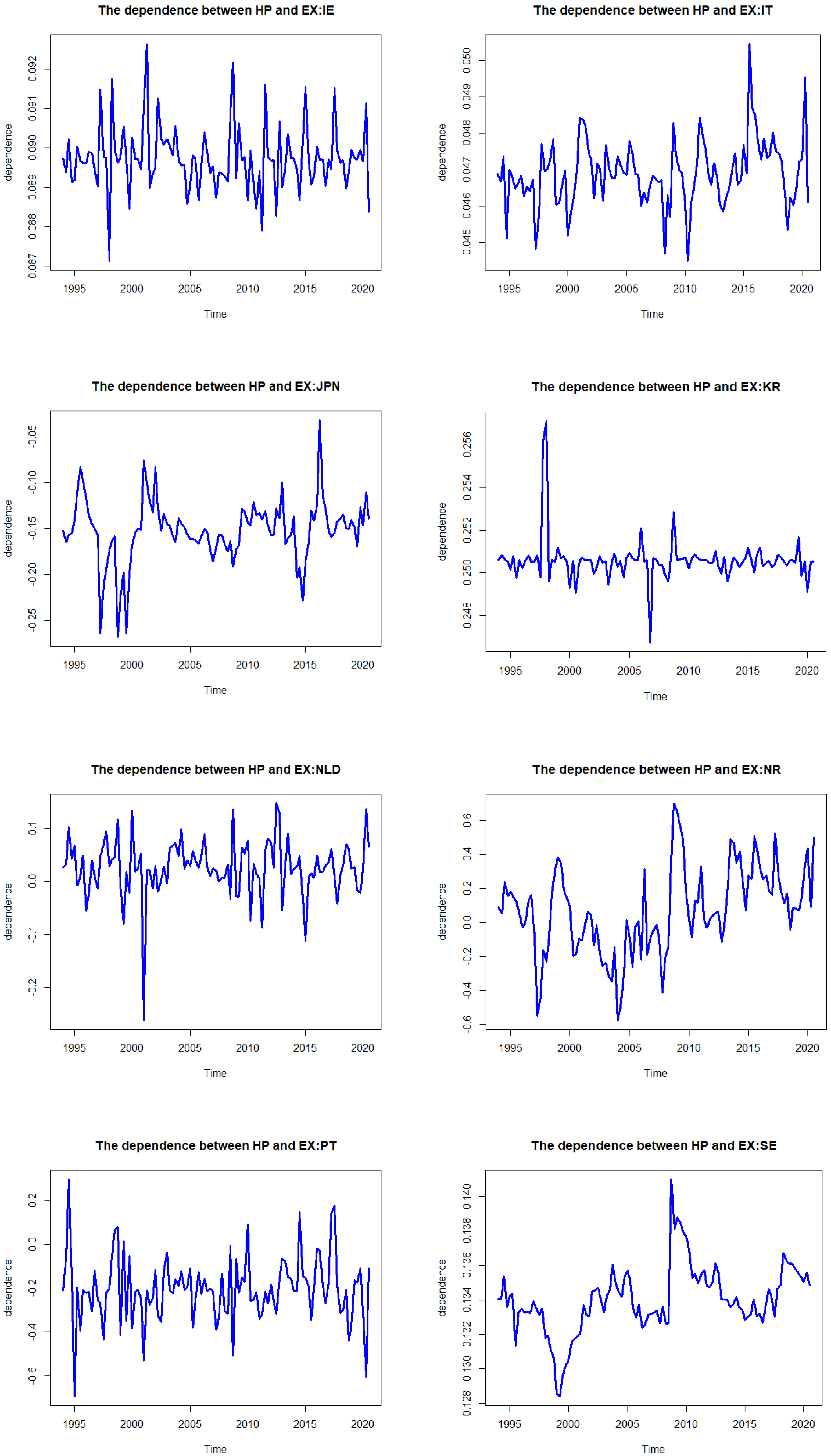
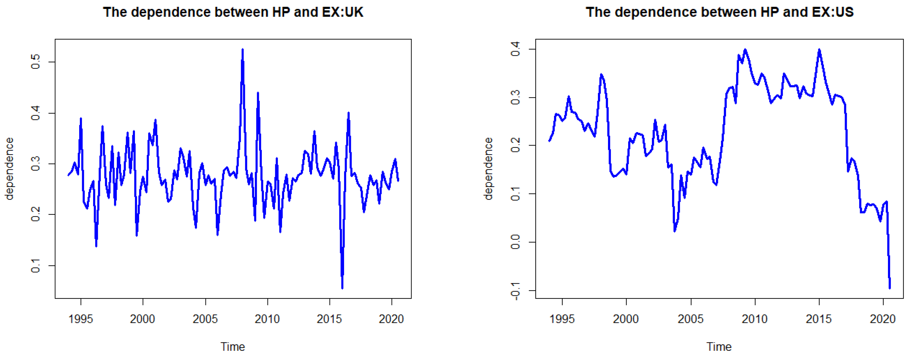
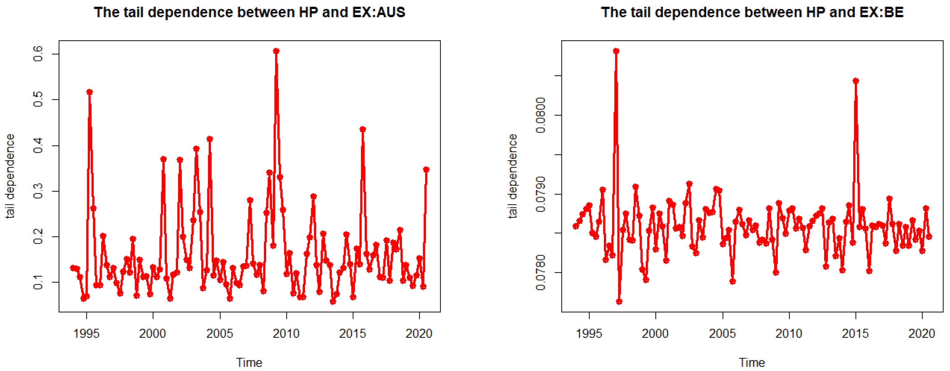
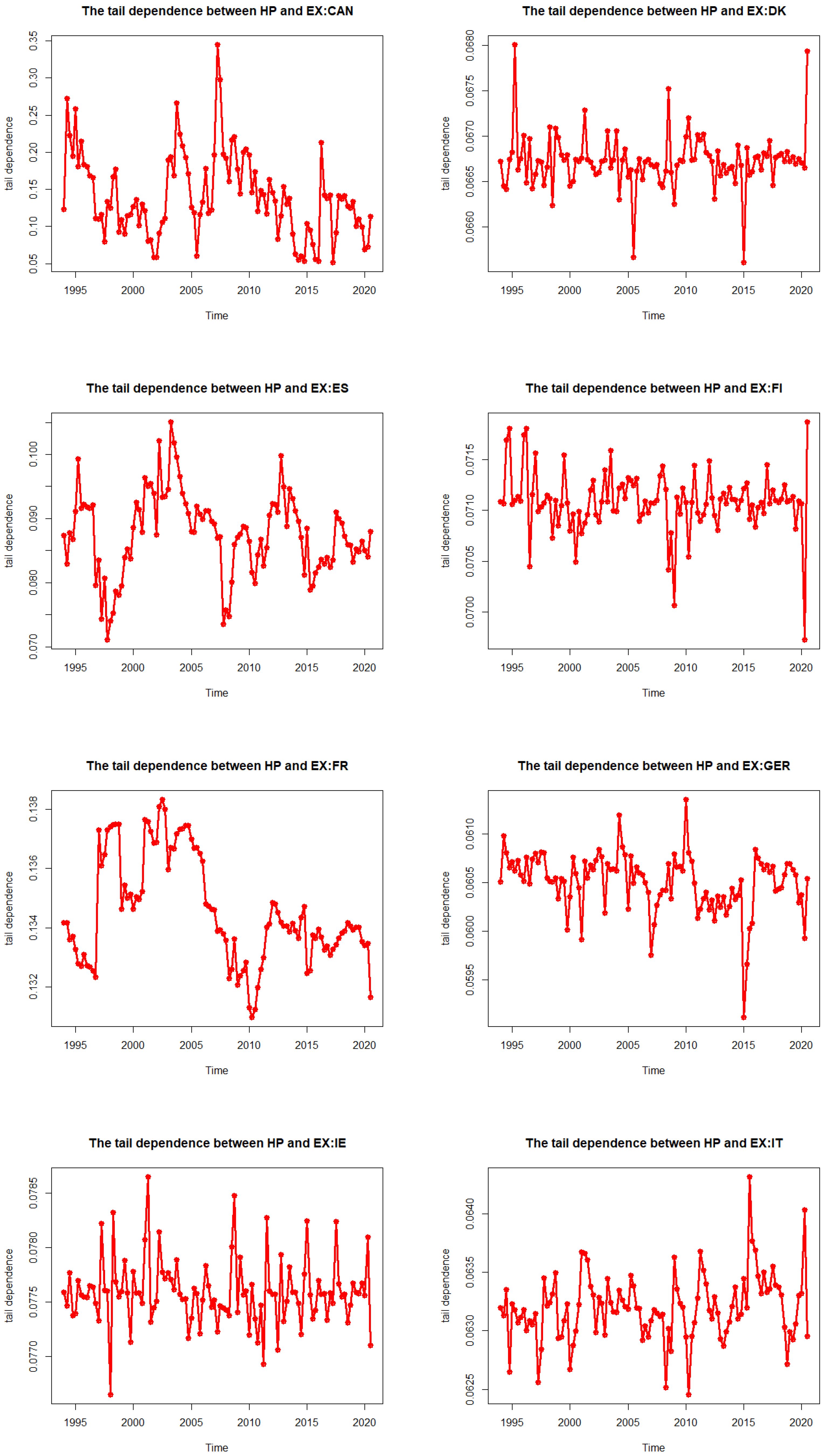
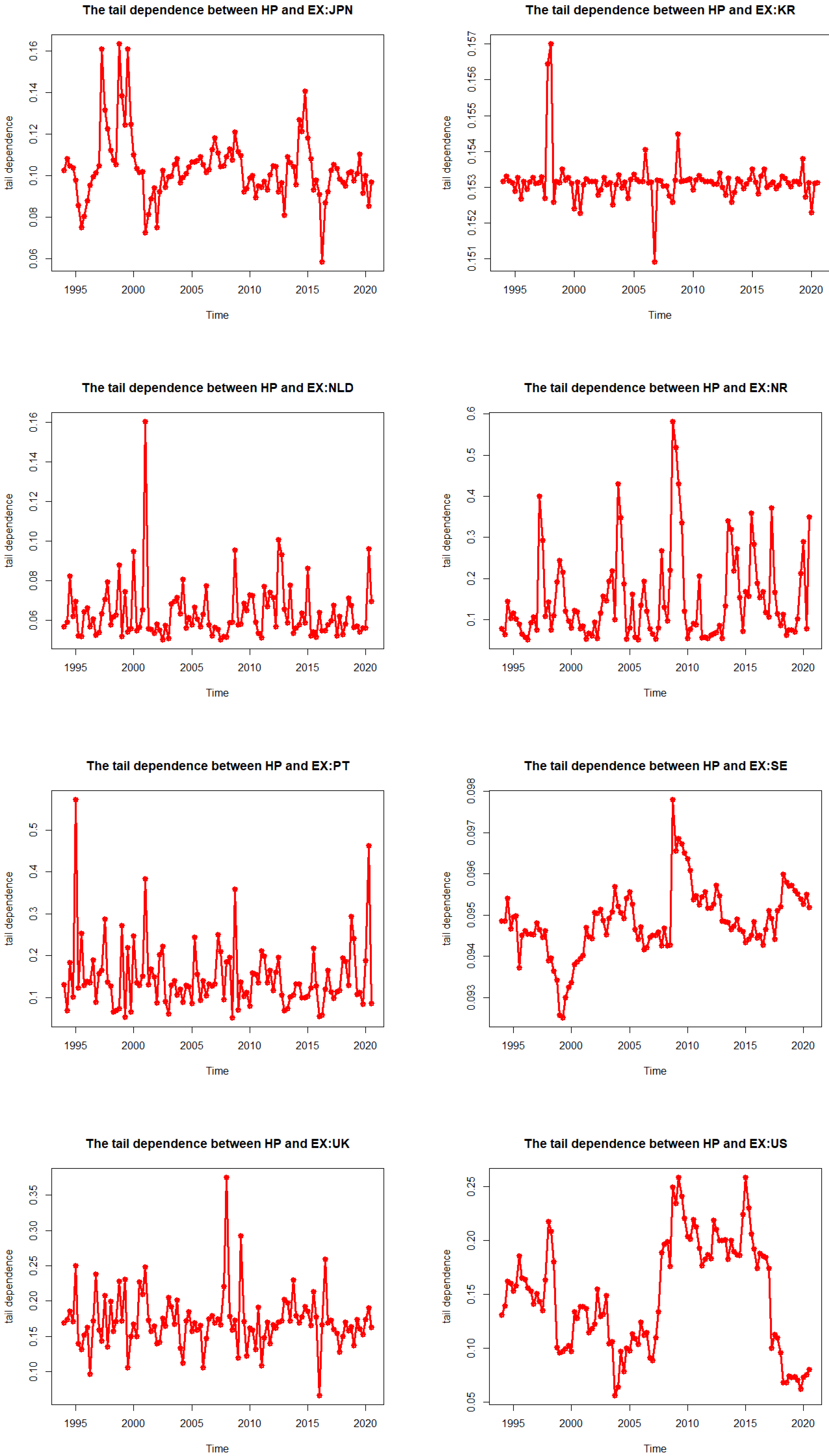
In addition, we hypothesized that the correlation between house prices and exchange rates may not be constant over time. To confirm our expectations and our hypothesis, we have plotted the time-varying nature of the dependence and tail dependence in Figure 1 and Figure 2, respectively.
Figure 1 shows the time-varying dependence between house prices and exchange rates in 18 OECD countries in the period 1994Q1–2020Q4. The dependence of most countries (11 out of 18) fluctuates around their average values. In other words, the dependence of these 11 countries is more stationary than the other seven countries. Among them, the time-varying dependences of Germany and Japan show a gradual change, while those of Australia, Belgium, Denmark, Finland, Ireland, Korea, The Netherlands, Portugal, and the UK present a swing movement.
The other seven countries exhibit time-varying dependence that does not fluctuate around their average value. Among them, Canada, France, Norway, Spain, and the USA have a weak fluctuation, while Italy presents a relatively greater fluctuation.
Considering the degree of dependence, a value larger/smaller than 0 indicates a positive/negative correlation between house prices and exchange rates, respectively. We find that the values of time-varying dependence between housing prices and exchange rates are mostly positive for the OECD countries in the sample period.
Interestingly, both positive and negative values are found in the cases of Australia, Canada, Japan, the Netherlands, Norway, Portugal, and the USA, indicating the existence of both positive and negative correlations between house prices and exchange rates. The negative values were found in two time periods: from 2000 to 2005 and 2015 to 2020. We find that the real effective exchange rates of these eight countries decreased, while house prices increased during these periods.
Figure 2 presents the time-varying tail dependence between house prices and exchange rates in the OECD countries. Along the sample period, the tail dependence of most countries (14 out of 18) has a high fluctuation but with movements around the mean, indicating that the time-varying tail dependence is quite stable. Among the remaining four countries, Spain has a high tail dependence fluctuation, while the fluctuation of France, Sweden, and the USA is quite weak. In terms of effect, the estimated values of tail dependence are greater than 0 between 1995 and 2020 for all countries. This means there is always a contagion between house prices and exchange rates in the extreme market episodes. The degree of tail dependence is relatively high around 1997–1998 and 2008–2009, corresponding to the Asian financial crisis and the subprime mortgage crisis in 2008. The possible reason is that, during the crisis period, investors seek to diversify their losses by selling some of their assets and purchasing other new assets. This fact allows for the contagion effects between house prices and exchange rates [39]. Our study highlights the challenges of market risk during economic downturns and the danger of under-predicting risk if time-varying dependence is ignored.
Comparing Figure 1 and Figure 2, the tail dependence has a smaller amplitude but higher fluctuation than the normal dependence. This indicates that the relationship between house prices and exchange rates of OECD countries is not stable in either normal or extreme market situations. However, the degree of dependence in the normal market is stronger than in the extreme markets [40].

4. Conclusions and Discussion

This empirical study employed quantile Granger causality and DCC copula GARCH to examine the causality and dependence between exchange rates and house prices in the OECD countries in the cycle of boom-and-bust markets during 1994Q1–2020Q4.
Overall, the results of the quantile Granger causality test revealed that in most cases there was a bidirectional Granger causality between house prices and exchange rates in OECD countries. In the bust market, we found no Granger causality between exchange rates and house prices in the UK; a unilateral one in Belgium, Finland, France, Germany, Norway, and the USA; and a bidirectional one elsewhere. In the boom market, there was no Granger causality between exchange rates and house prices in Australia; a unilateral one in Canada, Spain, and the Netherlands; and a bidirectional one in the remaining countries. Our mixed results from this study are similar to the findings of Bahmani-Oskooee and Wu [3], who found a consistently mixed relationship between oil and housing prices in OECD economies. However, our study provides more solid evidence that the mixed causality between housing markets and foreign exchange markets also occurs in the boom-and-bust market setting. This indicates that the direction of causality between real estate and the foreign exchange markets of the OECD may be determined by various factors that are country-specific.
The results of the DCC copula GARCH model estimation showed that there was a positive correlation between house prices and exchange rates in some OECD countries between 1995–2020. However, the time-varying dependences between house prices and exchange rates in Australia, Belgium, Japan, the Netherlands, Norway, Portugal, and the United States of America showed negative values in some subperiods, particularly 2000–2005 and 2015–2020. Then, the estimated dependence was further used for calculating the time-varying tail dependence. This enabled us to investigate the house price and exchange rate nexus in extreme events. The results showed that there is always contagion between exchange rates and house prices in the 18 OECD countries, as the degree of tail dependences of all pairs varied above the 0 value throughout the sample period. This implies that the two markets are likely to crash together. Therefore, any severe instability in one market is likely to coincide with turmoil in the other [2]. Considering that the average tail dependence value is smaller than the average dependence value in all countries except for Germany, we may conclude that the contagion between house prices and exchange rates becomes weaker in extreme markets. As pointed out by Lucarelli, Andrini, and Bianchi [41] and Gobbi and Lucarelli [42], Germany tends to reduce its foreign trade in periods of currency depreciation and in periods of depreciation the peripheral Eurozone economies always increase their integration with the German economic system. The inflationary effects of currency depreciation can spread to housing markets and push house prices higher. However, the degree of transmission depends on how dependent a country is on imported materials that are used in the construction business. In the case of Germany, the inflationary dynamics in house prices that are concentrated in the peripheral countries of the Eurozone may have been transmitted to the German house market with more vigor, precisely in the phases of depreciation of the Euro that favored imports from the European peripheries to Germany.
According to the above results, we suggest that OECD governments control extreme housing prices by lowering exchange rates, and likewise, that extreme exchange rates be controlled by lowering house prices. In addition, as the lag variable was used in the quantile Granger causality test, governments and investors can use house prices to predict exchange rates, and vice versa. Moreover, our results suggest that the increased contagion effect between house prices and exchange rates during financial crises will erode diversification benefits; therefore, institutions and investors should be aware of this contagion effect and consider other assets to diversify their risks. Last but not least, policymakers in the OECD community should remain observant of the extreme comovement between exchange rates and house prices and intervene when necessary to ensure price stability.
Some limitations of this article may become directions for future work. Firstly, we used quarterly data, while monthly or daily data could help to better understand the conversion or transformation of time series. Future research could collect monthly or daily data to better capture the changes in the causality and correlation between house prices and exchange rates. Secondly, because the variables analyzed in this article were confined to exchange rates and macroeconomic factors, future research could introduce other control variables such as interest rates, gross domestic product, government policies, and population growth in the 18 OECD countries. From a methodological perspective, our DCC copula GARCH relied on the Student-t distribution, and thus it may not be applicable when asymmetric tail dependence exists. Therefore, the use of mixed copula and asymmetric copulas is suggested in future studies [43].

Author Contributions

Conceptualization, W.Y. and M.L.; methodology, W.Y. and J.L.; software, W.Y. and J.L.; validation, P.M. and M.L.; formal analysis, W.Y. and M.L.; investigation, W.Y. and M.L. and H.Q.D.; data curation, M.L.; writing—original draft preparation, W.Y. and M.L.; writing—review and editing W.Y. and P.M. All authors have read and agreed to the published version of the manuscript.

Funding

The Center of Excellence in Econometrics, Faculty of Economics, Chiang Mai University and the China-ASEAN High-Quality Development Research Center in Shandong University of Finance and Economics.

Data Availability Statement

The data were obtained from the National Statistical Office of Thailand and Thomson Reuter Data Stream.

Acknowledgments

The authors would like to thank Laxmi Worachai for her constructive comments that helped improve our paper. The paper was financially supported by the Center of Excellence in Econometrics, Faculty of Economics, Chiang Mai University and the China-ASEAN High-Quality Development Research Center in Shandong University of Finance and Economics.

Conflicts of Interest

The authors declare no conflict of interest.

References

  1. Chen, M.C.; Tsai, I.C.; Chang, C.O. House prices and household income: Do they move apart? Evidence from Taiwan. Habitat Int. 2007, 31, 243–256. [Google Scholar] [CrossRef]
  2. Bissoondeeal, R.K.; Tsiaras, L. Investigating the Links between UK House Prices and Share Prices with Copulas. J. Real Estate Financ. Econ. 2021, 1–30. [Google Scholar] [CrossRef]
  3. Bahmani-Oskooee, M.; Wu, T.P. Housing prices and real effective exchange rates in 18 OECD countries: A bootstrap multivariate panel Granger causality. Econ. Anal. Policy 2018, 60, 119–126. [Google Scholar] [CrossRef]
  4. Malpezzi, S. A simple error correction model of house prices. J. Hous. Econ. 1999, 8, 27–62. [Google Scholar] [CrossRef]
  5. Gete, P. Expectations and the housing boom and bust. An open economy view. J. Hous. Econ. 2020, 49, 101690. [Google Scholar] [CrossRef]
  6. Apergis, N. Housing prices and macroeconomic factors: Prospects within the European Monetary Union. Int. Real Estate Rev. 2003, 6, 63–74. [Google Scholar] [CrossRef]
  7. Gallin, J. The long-run relationship between house prices and income: Evidence from local housing markets. Real Estate Econ. 2006, 34, 417–438. [Google Scholar] [CrossRef] [Green Version]
  8. Mikhed, V.; Zemčík, P. Do house prices reflect fundamentals? Aggregate and panel data evidence. J. Hous. Econ. 2009, 18, 140–149. [Google Scholar] [CrossRef] [Green Version]
  9. Kim, S.W.; Bhattacharya, R. Regional housing prices in the USA: An empirical investigation of nonlinearity. J. Real Estate Financ. Econ. 2009, 38, 443–460. [Google Scholar] [CrossRef]
  10. Holly, S.; Pesaran, M.H.; Yamagata, T. A spatio-temporal model of house prices in the USA. J. Econom. 2010, 158, 160–173. [Google Scholar] [CrossRef]
  11. Zhou, J. Testing for cointegration between house prices and economic fundamentals. Real Estate Econ. 2010, 38, 599–632. [Google Scholar] [CrossRef]
  12. Abbott, A.; De Vita, G. Pairwise convergence of district-level house prices in London. Urban Stud. 2012, 49, 721–740. [Google Scholar] [CrossRef]
  13. Abbott, A.; De Vita, G. Testing for long-run convergence across regional house prices in the UK: A pairwise approach. Appl. Econ. 2013, 45, 1227–1238. [Google Scholar] [CrossRef] [Green Version]
  14. Ding, H.; Chong, T.T.L.; Park, S.Y. Nonlinear dependence between stock and real estate markets in China. Econ. Lett. 2014, 124, 526–529. [Google Scholar] [CrossRef] [Green Version]
  15. Batayneh, K.I.; Al-Malki, A.M. The relationship between house prices and stock prices in Saudi Arabia: An empirical analysis. Int. J. Econ. Financ. 2015, 7, 156–167. [Google Scholar] [CrossRef] [Green Version]
  16. Apergis, N.; Simo-Kengne, B.D.; Gupta, R.; Chang, T. The dynamic relationship between house prices and output: Evidence from US metropolitan areas. Int. J. Strateg. Prop. Manag. 2015, 19, 336–345. [Google Scholar] [CrossRef] [Green Version]
  17. Gete, P.; Reher, M. Mortgage supply and housing rents. Rev. Financ. Stud. 2018, 31, 4884–4911. [Google Scholar] [CrossRef]
  18. Aizenman, J.; Jinjarak, Y. Real estate valuation, current account and credit growth patterns, before and after the 2008–9 crisis. J. Int. Money Financ. 2014, 48, 249–270. [Google Scholar] [CrossRef] [Green Version]
  19. Thomas, M.; Lee, S. The impact of exchanges rates on international real estate portfolio allocation. J. Real Estate Portf. Manag. 2006, 12, 277–292. [Google Scholar] [CrossRef]
  20. Yang, L.I.U.; Zhiqiang, H.U. On correlation between RMB exchange rate and real estate price based on financial engineering. Syst. Eng. Procedia 2012, 3, 146–152. [Google Scholar] [CrossRef]
  21. Sumer, L.; Özorhon, B. The exchange rate effect on housing price index and REIT index return rates. Finans. Araştırmalar Çalışmalar Derg. 2020, 12, 249–266. [Google Scholar] [CrossRef]
  22. Kónya, L. Exports and growth: Granger causality analysis on OECD countries with a panel data approach. Econ. Model. 2006, 23, 978–992. [Google Scholar] [CrossRef]
  23. Lipscomb, J.; Harvey, J.; Hunt, H. Exchange-rate risk mitigation with price-level-adjusting mortgages: The case of the Mexican UDI. J. Real Estate Res. 2003, 25, 23–42. [Google Scholar] [CrossRef]
  24. Troster, V. Testing for Granger-causality in quantiles. Econom. Rev. 2018, 37, 850–866. [Google Scholar] [CrossRef]
  25. Shafiullah, M.; Chaudhry, S.M.; Shahbaz, M.; Reboredo, J.C. Quantile causality and dependence between crude oil and precious metal prices. Int. J. Financ. Econ. 2021, 26, 6264–6280. [Google Scholar] [CrossRef]
  26. Li, R.; Li, S.; Yuan, D.; Zhu, H. Investor attention and cryptocurrency: Evidence from wavelet-based quantile Granger causality analysis. Res. Int. Bus. Financ. 2021, 56, 101389. [Google Scholar] [CrossRef]
  27. Kim, J.M.; Jung, H. Linear time-varying regression with Copula–DCC–GARCH models for volatility. Econ. Lett. 2016, 145, 262–265. [Google Scholar] [CrossRef]
  28. Demarta, S.; McNeil, A.J. The t copula and related copulas. Int. Stat. Rev. 2005, 73, 111–129. [Google Scholar] [CrossRef]
  29. Zellner, A. An efficient method of estimating seemingly unrelated regressions and tests for aggregation bias. J. Am. Stat. Assoc. 1962, 57, 348–368. [Google Scholar] [CrossRef]
  30. Bollerslev, T. Generalized autoregressive conditional heteroskedasticity. J. Econom. 1986, 31, 307–327. [Google Scholar] [CrossRef] [Green Version]
  31. Sklar, A. Random variables, joint distribution functions, and copulas. Kybernetika 1973, 9, 449–460. [Google Scholar]
  32. Engle, R. Dynamic conditional correlation: A simple class of multivariate generalized autoregressive conditional heteroskedasticity models. J. Bus. Econ. Stat. 2002, 20, 339–350. [Google Scholar] [CrossRef]
  33. Tse, Y.K.; Tsui, A.K.C. A multivariate generalized autoregressive conditional heteroscedasticity model with time-varying correlations. J. Bus. Econ. Stat. 2002, 20, 351–362. [Google Scholar] [CrossRef]
  34. Nagler, T.; Czado, C. Evading the curse of dimensionality in nonparametric density estimation with simplified vine copulas. J. Multivar. Anal. 2016, 151, 69–89. [Google Scholar] [CrossRef] [Green Version]
  35. Tang, M.L.; Bentler, P.M. Maximum likelihood estimation in covariance structure analysis with truncated data. Br. J. Math. Stat. Psychol. 1997, 50, 339–349. [Google Scholar] [CrossRef]
  36. Cortese, F.P. Tail dependence in financial markets: A dynamic copula approach. Risks 2019, 7, 116. [Google Scholar] [CrossRef] [Green Version]
  37. Alqahtani, F.; Trabelsi, N.; Samargandi, N.; Shahzad, S.J.H. Tail Dependence and Risk Spillover from the US to GCC Banking Sectors. Mathematics 2020, 8, 2055. [Google Scholar] [CrossRef]
  38. Zimmer, D.M. Time-varying correlation in housing prices. J. Real Estate Financ. Econ. 2015, 51, 86–100. [Google Scholar] [CrossRef]
  39. Maneejuk, P.; Yamaka, W. Predicting contagion from the US financial crisis to international stock markets using dynamic copula with google trends. Mathematics 2019, 7, 1032. [Google Scholar] [CrossRef] [Green Version]
  40. Pastpipatkul, P.; Yamaka, W.; Sriboonchitta, S. Dependence structure of and co-movement between Thai currency and international currencies after introduction of quantitative easing. In Causal Inference in Econometrics; Springer: Cham, Switzerland, 2016; pp. 545–564. [Google Scholar]
  41. Lucarelli, S.; Andrini, F.U.; Bianchi, A. Euro depreciation and trade asymmetries between Germany and Italy versus the US: Industry-level estimates. Appl. Econ. 2018, 50, 15–34. [Google Scholar] [CrossRef]
  42. Gobbi, L.; Lucarelli, S. ECB quantitative easing, euro depreciation and supply chains: Industry-level estimates for Germany, Italy and Greece. New prospects for a Minskyan big bank? PSL Q. Rev. 2021, 74, 15–50. [Google Scholar]
  43. Maneejuk, P.; Yamaka, W.; Sriboonchitta, S. Mixed-copulas approach in examining the relationship between oil prices and ASEAN’s stock markets. In Proceedings of the International Econometric Conference of Vietnam, Ho Chi Minh, Vietnam, 15–16 January 2018; Springer: Cham, Switzerland, 2018; pp. 531–541. [Google Scholar]
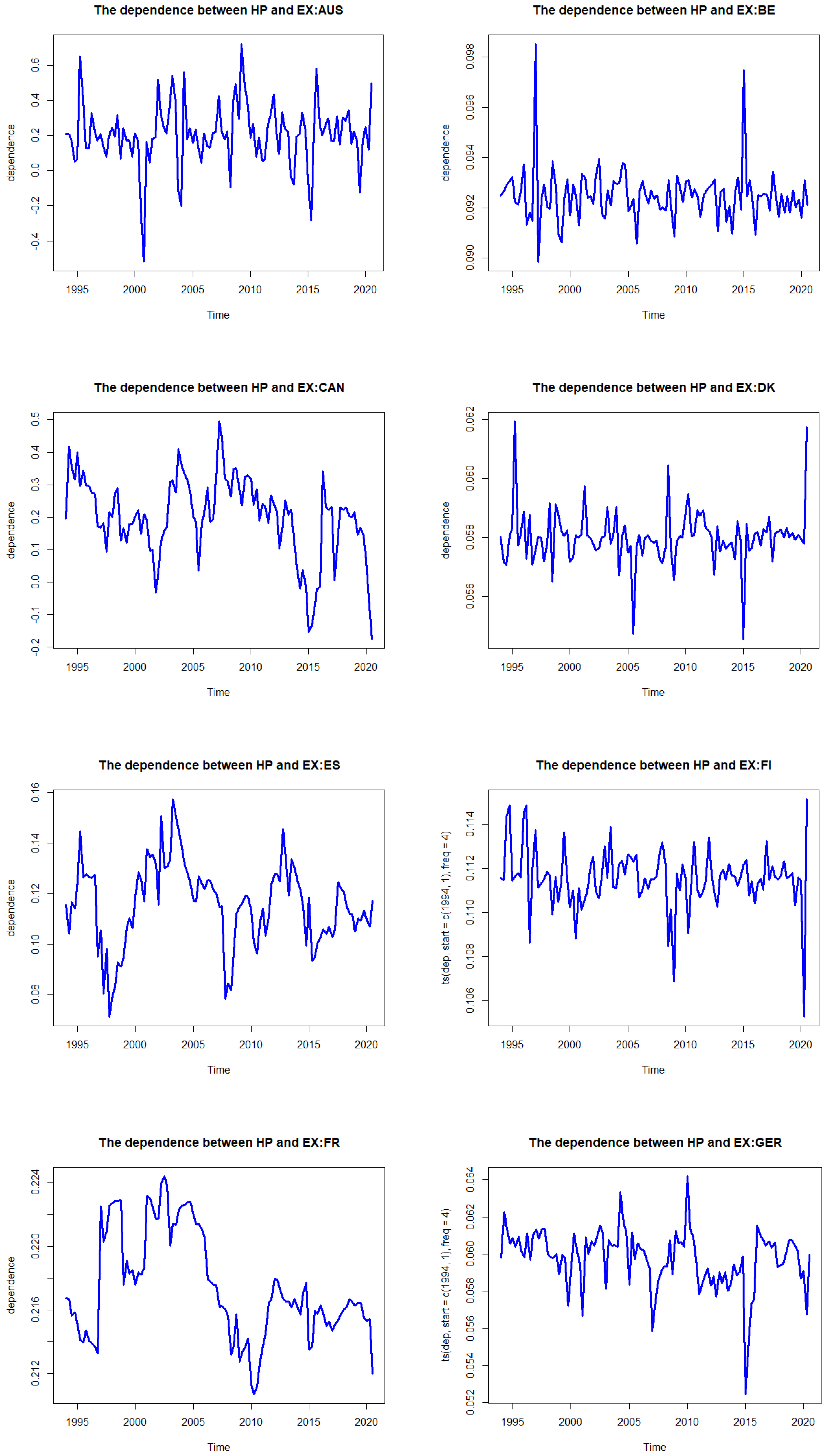
Figure 1. The dependence between house prices and exchange rates in OECD countries.
Axioms 11 00113 g001aAxioms 11 00113 g001bAxioms 11 00113 g001c
Figure 2. The tail dependence between house prices and exchange rates for OECD countries.
Axioms 11 00113 g002aAxioms 11 00113 g002bAxioms 11 00113 g002c
Table 1. Descriptive statistics of the real effective exchange rate index of OECD countries.
VariableMaxMinMeanSkewKurtStd.DevADFp-Value
Australia120.84872.95594.3890.234−0.77012.838−8.3950.000
Belgium111.05895.254103.711−0.4800.1663.192−7.6270.000
Canada126.72387.319103.6080.500−1.00210.735−8.6820.000
Denmark110.89897.291103.8080.257−0.4942.964−8.3250.000
Spain110.96592.976101.621−0.193−1.0034.670−6.2100.000
Finland119.98298.518105.4901.05481.2254.540−7.7390.000
France120.36699.406108.7190.150−1.0505.627−7.5340.000
Germany130.24099.065110.2830.752−0.0317.381−8.1400.000
Ireland129.49491.610106.2460.638−0.3818.759−7.3000.000
Italy110.74190.253103.993−0.3220.1753.943−8.1130.000
Japan213.34698.582139.6730.378−0.55026.527−4.9290.001
Korea119.52269.53699.5550.0110.0749.912−8.7930.000
Netherlands110.70894.722104.027−0.131−0.6263.673−8.1260.000
Norway126.35189.921110.854−0.570−0.1637.516−9.5640.000
Portugal106.75894.534101.467−0.179−0.8722.953−9.6710.000
Sweden137.77690.436112.2540.083−0.52811.368−8.1350.000
UK115.6983.07898.8680.121−1.59110.669−7.1770.000
USA116.22884.59699.1310.086−0.9598.116−7.9500.000
Table 2. Descriptive statistics of the housing price index of OECD countries.
VariableMaxMinMeanSkewKurtStd.DevADFp-Value
Australia112.17940.14874.937−0.136−1.25923.278−4.8690.000
Belgium110.80053.83285.191−0.447−1.44518.479−3.6910.000
Canada133.80048.07778.4260.489−1.00126.360−5.2720.000
Denmark121.96546.88888.228−0.253−1.07121.957−3.7800.000
Spain165.87469.145108.6570.301−1.00628.799−3.4940.000
Finland105.90056.31588.791−0.776−0.85415.853−4.0610.000
France114.00050.69786.695−0.526−1.50722.641−2.9350.000
Germany133.10087.800101.4540.9490.54210.492−8.9660.000
Ireland160.80046.900103.179−0.159−0.79130.737−3.4940.000
Italy136.35085.067107.8440.400−1.16915.418−10.4350.000
Japan146.01792.900111.7820.816−0.83416.292−4.2160.001
Korea112.52272.84094.370−0.875−0.1489.052−4.6280.000
Netherlands134.10056.552104.868−0.944−0.18820.939−3.4940.000
Norway110.10032.0073.843−0.1621.34224.906−6.0550.000
Portugal144.80093.300120.694−0.398−0.78013.672−3.4940.000
Sweden123.30035.54973.5180.096−1.21126.440−4.8870.000
UK112.30038.90082.271−0.655−1.05924.405−4.3630.000
US127.80073.90096.6870.115−1.05414.926−3.4930.000
Table 3. The LLC panel unit root test results.
VariableMaxMinMeanSkewKurtStd.DevLLCp-Value
E X 124.31690.558105.9830.133−0.4668.077−5.9930.000
H P 128.09560.04593.413−0.120−0.75020.258−8.2340.000
R G D P 62,991.9125,384.0935,024.32−0.2332.2284943.922−4.0830.000
I 22.8320.07321.9080.8302.7682.739−5.0310.000
Table 4. The results of quantile Granger causality between housing prices and exchange rates in the boom market in OECD countries (quantile = 0.9).
CountryGEX Cause GHPGHP Cause GEX
p-ValueCausalityp-ValueCausality
Australia0.121Yes0.211Yes
Belgium0.023No0.301Yes
Canada0.121Yes0.108Yes
Denmark0.503Yes0.232Yes
Spain0.221Yes0.122Yes
Finland0.343Yes0.003No
France0.245Yes0.005No
Germany0.434Yes0.003No
Ireland0.107Yes0.293Yes
Italy0.201Yes0.193Yes
Japan0.105Yes0.762Yes
Korea0.321Yes0.201Yes
Netherlands0.294Yes0.184Yes
Norway0.056No0.501Yes
Portugal0.301Yes0.211Yes
Sweden0.104Yes0.401Yes
UK0.000No0.000No
USA0.000No0.329Yes
Table 5. The results of quantile Granger causality between housing prices and exchange rates in the bust market in OECD countries (quantile = 0.1).
CountryGEX Cause GHPGHP Cause GEX
p-ValueCausalityp-ValueCausality
Australia0.000No0.008No
Belgium0.344Yes0.490Yes
Canada0.108Yes0.000No
Denmark0.693Yes0.390Yes
Spain0.000No0.440Yes
Finland0.202Yes0.842Yes
France0.839Yes0.108Yes
Germany0.224Yes0.421Yes
Ireland0.409Yes0.213Yes
Italy0.156Yes0.224Yes
Japan0.772Yes0.302Yes
Korea0.394Yes0.221Yes
Netherlands0.000No0.209Yes
Norway0.834Yes0.200Yes
Portugal0.247Yes0.498Yes
Sweden0.690Yes0.702Yes
UK0.509Yes0.287Yes
USA0.873Yes0.654Yes
Table 6. The results of quantile Granger causality between housing prices and exchange rates in the normal market in OECD countries (quantile = 0.5).
CountryGEX Cause GHPGHP Cause GEX
p-ValueCausalityp-ValueCausality
Australia0.023No0.223Yes
Belgium0.001No0.824Yes
Canada0.774Yes0.002No
Denmark0.002No0.001No
Finland0.292Yes0.229Yes
France0.301Yes0.493Yes
Germany0.224Yes0.000No
Ireland0.092No0.254Yes
Italy0.392Yes0.119Yes
Japan0.743Yes0.394Yes
Korea0.224Yes0.320Yes
Netherlands0.302Yes0.983Yes
Norway0.924Yes0.291Yes
Portugal0.000No0.390Yes
Spain0.021No0.000No
Sweden0.091No0.083No
UK0.000No0.000No
USA0.345Yes0.011No
Table 7. The results of GARCH (1,1) for exchange rate.
Parameterμ φ 0 φ 1 ϑ 1 Log-
Likelihood
Q (1)ARCH (1)-LM
Australia
 
Belgium
 
Canada
 
Denmark
 
Spain
 
Finland
 
France
 
Germany
 
Ireland
 
Italy
 
Japan
 
Korea
 
Netherlands
 
Norway
 
Portugal
 
Sweden
 
UK
 
USA
 
0.001 *
(0.001)
0.000 *
(0.001)
0.000 *
(0.001)
0.000 *
(0.001)
0.000 *
(0.000)
0.000 *
(0.000)
0.001 *
(0.001)
−0.001 *
(0.001)
0.000 *
(0.001)
0.000 *
(0.001)
−0.003 *
(0.002)
0.002 *
(0.001)
0.000 *
(0.001)
−0.001 *
(0.001)
0.000 *
(0.000)
−0.001 *
(0.001)
−0.001 *
(0.001)
0.000 *
(0.001)
0.000 *
(0.000)
0.000 *
(0.000)
0.000 *
(0.000)
0.000 *
(0.000)
0.000 *
(0.000)
0.000 *
(0.000)
0.000 *
(0.000)
0.000 *
(0.000)
0.000 *
(0.000)
0.000 *
(0.000)
0.000 *
(0.000)
0.000 *
(0.000)
0.000 *
(0.000)
0.000 *
(0.000)
0.000 *
(0.000)
0.000 *
(0.000)
0.000 *
(0.000)
0.000 *
(0.000)
0.001 *
(0.013)
0.006 *
(0.028)
0.277 *
(0.179)
0.004 *
(0.044)
0.001 *
0.002
0.115 *
(0.326)
0.001 *
(0.002)
0.000 *
(0.001)
0.000 *
(0.001)
0.263 *
(0.097)
0.000 *
(0.014)
0.467 *
(0.547)
0.000 *
(0.001)
0.000 *
(0.007)
0.006 *
(0.019)
0.000 *
(0.000)
0.000 *
(0.008)
0.000 *
(0.005)
0.996 *
(0.015)
0.990 *
(0.032)
0.583 *
(0.174)
0.993 *
(0.050)
0.997 *
0.002
0.840 *
(0.357)
0.998 *
(0.002)
0.998 *
(0.001)
0.998 *
(0.001)
0.562 *
(0.090)
0.995 *
(0.018)
0.264 *
(0.275)
0.997 *
(0.001)
0.999 *
(0.006)
0.989 *
(0.022)
0.998 *
(0.000)
0.999 *
(0.007)
0.999 *
(0.005)
300.745
 
428.020
 
331.006
 
415.697
 
420.142
 
399.687
 
425.977
 
397.402
 
378.668
 
404.200
 
288.104
 
308.411
 
399.928
 
336.605
 
463.464
 
339.252
 
342.664
 
347.242
 
0.915
 
0.814
 
0.739
 
0.994
 
0.462
 
0.484
 
0.618
 
0.752
 
0.340
 
0.963
 
0.846
 
0.379
 
0.757
 
0.376
 
0.215
 
0.136
 
0.758
 
0.654
 
0.564
 
0.511
 
0.720
 
0.139
 
0.359
 
0.334
 
0.791
 
0.174
 
0.609
 
0.508
 
0.668
 
0.640
 
0.712
 
0.804
 
0.454
 
0.942
 
0.937
 
0.550
 
Note: () denotes standard error and “*” stands for statistical significance at the 5% level. Q (1) is the Ljung–Box Q statistic for the null hypothesis that there is no autocorrelation up to order 1 for the standardized residuals.
Table 8. The results of GJR-GARCH (1,1) for housing price.
Parameterμ φ 0 φ 1 ϑ 1 Log-LikelihoodQ (1)ARCH (1)-LM
Australia
 
Belgium
 
Canada
 
Denmark
 
Spain
 
Finland
 
France
 
Germany
 
Ireland
 
Italy
 
Japan
 
Korea
 
Netherlands
 
Norway
 
Portugal
 
Sweden
 
UK
 
USA
 
0.004 *
(0.002)
0.003 *
(0.000)
0.004 *
(0.001)
0.004 *
(0.001)
−0.002 *
(0.004)
0.000 *
(0.001)
−0.003 *
(0.002)
−0.001 *
(0.001)
0.002 *
(0.005)
−0.008 *
(0.002)
−0.002 *
(0.001)
0.000 *
(0.000)
0.005 *
(0.003)
0.005 *
(0.001)
−0.001 *
(0.002)
0.005 *
(0.001)
0.004 *
(0.002)
0.004 *
(0.002)
0.000 *
(0.000)
0.000 *
(0.000)
0.000 *
(0.000)
0.000 *
(0.000)
0.000 *
(0.000)
0.000 *
(0.000)
0.000 *
(0.000)
0.000 *
(0.000)
0.000 *
(0.000)
0.000 *
(0.000)
0.000 *
(0.000)
0.000 *
(0.000)
0.000 *
(0.000)
0.000 *
(0.000)
0.000 *
(0.000)
0.000 *
(0.000)
0.000 *
(0.000)
0.000 *
(0.000)
0.000 *
(0.010)
0.008 *
(0.022)
0.456 *
(0.207)
0.346
(0.180)
0.223 *
(0.098)
0.589 *
(0.297)
0.475 *
(0.208)
0.169 *
(0.038)
0.148 *
(0.055)
0.354 *
(0.177)
0.314 *
(0.151)
0.165 *
(0.134)
0.090 *
(0.025)
0.220 *
(0.0701)
0.000 *
(0.024 *)
0.000 *
(0.007)
0.389 *
(0.138)
0.265 *
(0.116)
0.995 *
(0.011)
0.985 *
(0.027)
0.543 *
(0.144)
0.477
0.123
0.665 *
(0.057)
0.410 *
(0.073)
0.463 *
(0.034)
0.763 *
(0.062)
0.741 *
(0.069)
0.398 *
(0.133)
0.685 *
(0.097)
0.834 *
(0.069)
0.664 *
(0.061)
0.638 *
(0.085)
0.999 *
(0.018)
0.999 *
(0.007)
0.610 *
(0.110)
0.706 *
(0.095)
404.508
 
424.184
 
425.671
 
409.341
 
413.902
 
422.550
 
466.536
 
429.898
 
361.837
 
468.160
 
484.814
 
434.012
 
447.000
 
392.873
 
425.741
 
417.912
 
404.876
 
504.900
 
0.069
 
0.061
 
0.399
 
0.565
 
0.684
 
0.622
 
0.899
 
0.819
 
0.725
 
0.717
 
0.806
 
0.889
 
0.507
 
0.722
 
0.858
 
0.735
 
0.981
 
0.775
 
0.195
 
0.400
 
0.776
 
0.624
 
0.843
 
0.649
 
0.845
 
0.863
 
0.692
 
0.590
 
0.808
 
0.968
 
0.922
 
0.857
 
0.586
 
0.644
 
0.571
 
0.743
 
Note: () denotes standard error and “*” stands for statistical significance at the 5% level. Q (1) is the Ljung–Box Q statistic for the null hypothesis that there is no autocorrelation up to order 1 for the standardized residuals.
Table 9. The results of the DCC copula part.
Country CoefSEp-ValueMean (Dep)Mean (Tail)
Australiaa0.2520.1170.0320.3550.160
b0.0010.0011.000
Belgiuma0.0010.0110.9290.1450.079
b0.0010.0011.000
Canadaa0.1100.0960.2520.3250.140
b0.6550.3740.080
Denmarka0.0010.0620.9880.0910.067
b0.0010.0011.000
Spaina0.0120.0740.8710.1810.088
b0.7530.4930.127
Finlanda0.0010.0260.9700.1120.071
b0.0010.0011.000
Francea0.0020.0360.9670.3350.135
b0.9240.0011.000
Germanya0.0010.1530.9950.0600.061
b0.6117.3540.934
Irelanda0.0010.0011.0000.1400.076
b0.0010.0011.000
Italya0.0010.1410.9940.0740.063
b0.4495.4840.935
Japana0.0440.1960.8210.2360.103
b0.5670.5940.339
Koreaa0.0010.0740.9890.3840.153
b0.00113.2901.000
Netherlandsa0.0590.1030.5710.0710.064
b0.0010.0011.000
Norwaya0.2330.1120.0370.3100.150
b0.4970.2580.054
Portugala0.2230.1590.1590.3360.149
b0.0010.3820.998
Swedena0.0010.0460.9830.2090.095
b0.8551.5250.575
UKa0.0810.0011.0000.4190.172
b0.0010.0011.000
USAa0.0470.0430.2730.3520.149
b0.8810.0011.000
DCC-Copula (Normal Copula)    AIC = 278.829    BIC = 300.092
CCC-Copula (Normal Copula)    AIC = 293.093    BIC = 317.023
DCC-Copula (Student-t Copula)    AIC = 257.098    BIC = 280.189
CCC-Copula (Student-t Copula) AIC = 285.229 BIC = 302.109
Note: dep and tail stand for dependence and tail dependence between house price and exchange rate. CCC stands for constant conditional correlation model.
Publisher’s Note: MDPI stays neutral with regard to jurisdictional claims in published maps and institutional affiliations.