Article

RainPredRNN: A New Approach for Precipitation Nowcasting with Weather Radar Echo Images Based on Deep Learning

1
School of Information and Communication Technology, Hanoi University of Science and Technology, Hanoi 01000, Vietnam
2
Faculty of Computer Science and Engineering, Thuyloi University, Hanoi 10000, Vietnam
3
Faculty of Water Resources Engineering, Thuyloi University, Hanoi 10000, Vietnam
4
Department of Digital Systems, Faculty of Technology, University of Thessaly, Geopolis, 41500 Larissa, Greece
5
VNU Information Technology Institute, Vietnam National University, Hanoi 01000, Vietnam
*
Authors to whom correspondence should be addressed.
Axioms 2022, 11(3), 107; https://doi.org/10.3390/axioms11030107
Submission received: 3 January 2022 / Revised: 19 February 2022 / Accepted: 22 February 2022 / Published: 28 February 2022
(This article belongs to the Special Issue Various Deep Learning Algorithms in Computational Intelligence)

Abstract

:
Precipitation nowcasting is one of the main tasks of weather forecasting that aims to predict rainfall events accurately, even in low-rainfall regions. It has been observed that few studies have been devoted to predicting future radar echo images in a reasonable time using the deep learning approach. In this paper, we propose a novel approach, RainPredRNN, which is the combination of the UNet segmentation model and the PredRNN_v2 deep learning model for precipitation nowcasting with weather radar echo images. By leveraging the abilities of the contracting-expansive path of the UNet model, the number of calculated operations of the RainPredRNN model is significantly reduced. This result consequently offers the benefit of reducing the processing time of the overall model while maintaining reasonable errors in the predicted images. In order to validate the proposed model, we performed experiments on real reflectivity fields collected from the Phadin weather radar station, located at Dien Bien province in Vietnam. Some credible quality metrics, such as the mean absolute error (MAE), the structural similarity index measure (SSIM), and the critical success index (CSI), were used for analyzing the performance of the model. It has been certified that the proposed model has produced improved performance, about 0.43, 0.95, and 0.94 of MAE, SSIM, and CSI, respectively, with only 30% of training time compared to the other methods.

1. Introduction

Precipitation nowcasting from high-resolution radar data is essential in many branches such as water management, agriculture, aviation, emergency planning, and so on. It aims to make detailed and plausible predictions of future radar images based on past radar images with information about the amount, timing, and location of rainfall. This problem is significant to nowcasting the rainfall events in the next few hours with tropical depression in a given direction, entering from one area to another [1]. In such a case with heavy rainfall in the past few days, which is expected to continue to increase in the coming days, the prediction would help localities to ensure the safety of dams and essential dikes, to avoid unexpected flood discharges, causing flooding and inundation for the downstream area. According to the report on the assessment of disaster events in the 21st century implemented by the Centre for Research on the Epidemiology of Disasters [2], floods cause more negative impacts on people than any other natural catastrophe. Additionally, rain has a detrimental impact on travel demand and travel time, as well as on road traffic accidents, in metropolitan areas worldwide [3,4,5].
In recent years, deep learning has been applied to many areas [6,7,8]. Various variants of convolutional neural network (CNN) and recurrent neural network (RNN) architectures have been modified and applied in a variety of domains to produce suitable versions and solve specific problems [9,10,11,12]. Several studies on applications of deep learning for time-series data problems are briefly reviewed as follows.
Khiali et al. [13] presented a new approach that is a combination of graph-based techniques in order to design a new clustering framework for satellite time-series images. Spatiotemporal features are firstly extracted, which are then represented in their movements in the graph. Based on their similar characteristics, spatiotemporal clusters are produced. Since transmission lines often undergo various faults and errors, which caused terrible economic damage, Fahim et al. [14] proposed a robust self-attention CNN (SAT-CNN) that uses time-series image extracted features for detection and classification of faults. By adding the discrete wavelet transform (DWT) preprocessing method, the proposed model shows the superiority of the performance compared to others. Since in the traditional approaches of exploiting time-series, there may be human intervention in extracting features, Li et al. [15] introduced a novel approach that uses various computer vision algorithms in order to automatically extract features from time-series imagery after the images are transformed into recurrence plots. The method showed significant performance in two datasets: the largest forecasting competition dataset (M4) and the tourism forecasting competition dataset.
Precipitation nowcasting has attracted many researchers’ attention [16,17,18]. In recent years, computer vision with deep learning has shown dramatic promise. Agrawal et al. [19] applied one of the most popular models, UNet, in order to forecast precipitation and produced favorably comparable results. In 2021, Fernández and Mehrkanoon [20] used deep learning for weather nowcasting by presenting a novel UNet-based architecture model, Broad-UNet. To learn more complex abstract features of input images, this model alters convolution layers and pooling layers by asymmetric parallel convolutions and atrous spatial pyramid pooling (ASPP), respectively. Thus, the Broad-UNet model exhibits great performance compared to others. In order to support meteorologists nowcasting short-term weather with a large volume of satellite and radar images, Ionescu et al. [21] introduced the family of the CNN architecture, DeePS. By using five satellite products to collect satellite image data, the model was analyzed and compared with other CNN-based models and was found to reach a 3.84% MAE score for an entire dataset.
By applying deep learning methods in supporting meteorologists to predict future disastrous weather, Zhang et al. [22] proposed a high-performance model for predicting changes in weather radar echo shape, which is based on the combination of the conventional CNN and the long short-term memory (LSTM) network. In practice, their model produces significant results in various evaluation methods, such as the critical success index (CSI) and the Heidke skill score, compared to ConvLSTM and TrajGRU models. Trebing et al. [23] noticed that numerical weather prediction methods lack the ability for short-term forecasts using the latest available information. They introduced the application of deep learning in a novel comparable performance neural network, small attention UNet (SmaAt-UNet), which uses only 25% of the trainable network parameters. Additionally, Le et al. [24] firstly applied the LSTM neural network to perform flood forecasting on Da River in Vietnam. The suggested model was evaluated by the Nash–Sutcliffe efficiency (NSE) score in different prediction cases and produced considerably high performances (around 90% NSE). In 2021, Le et al. [25] also compared different deep learning models for forecasting river streamflow. Various state-of-the-art models were reviewed and evaluated, such as StackedLSTM and BiLSTM.
Although the above-mentioned articles have contributed considerably to the fields of forecasting and nowcasting by applying various state-of-the-art deep learning algorithms, few can manage and apply spatiotemporal and temporal features in both long- and short-term time-series imagery. However, in precipitation nowcasting, not enough studies are available that have applied time-series imagery to predict future scenes [26,27]. Recently, Wang et al. [28] released a deep learning model that has proven powerful in processing time-series image datasets. Despite the original model, PredRNN_v2 working well in most cases, we noticed that this model took a tremendous amount of time for training and testing (in terms of radar dataset), in particular if we want to retrain the model with a larger dataset later down the road. This describes the motivation for this paper, that is, to design a new deep learning method to improve the overall process and work well with multistep prediction.
Therefore, in this paper, we aim to introduce a novel deep learning approach in precipitation nowcasting with valuable collected radar datasets to overcome the above limitations. The proposed model is a combination of the power of UNet [29] and PredRNN_v2 [28] with the purpose of reducing training and testing time while preserving the complex spatial features of radar data. Our model benefits from the robustness of PredRNN_v2 in managing both spatiotemporal and temporal information of time-series images. Additionally, the contracting and expanding paths of UNet have a vital role in reducing the size of inputs, while it still captures the high-level features of original images.
In the implementation, we set up our case study to allow our model to have the ability to predict images following one hour (6 timesteps with a 10 min gap) so that the model still produces comparable performances. By such a design, the computation time of the training and testing phases of the proposed model is reduced remarkably, approximately 30% smaller than that of the original PredRNN_v2. In addition, our model produces impressive performances compared to others by evaluating it with various quality assessments.
The organization of the rest of the paper is as follows. Τhe data preparation and the background underlying the proposed model are described in Section 2. In Section 3, by leveraging the advantages of the encoder–decoder architecture, we introduce the most suitable model for solving the above-mentioned problems. In Section 4, we present the environment setup and the implementation served for the evaluation and the comparison of the suggested model with others, as well as discuss the comparison results. Finally, conclusions and future development directions are described in Section 5.

2. Data and Background

2.1. Background

2.1.1. Convolutional LSTM (ConvLSTM)

Since traditional standard LSTMs, which are special RNN architectures [30], have a significant drawback in simultaneously modeling the spatiotemporal information of inputs, the hidden states, and the output memory cells, the ConvLSTM [31] with various improvements can tackle the problem of the former version (FC-LSTM). First, in order to encode the spatial structure information, all the inputs X 1 ,   ,   X t , the output cells C 1 , , C t , and the hidden states H 1 ,   ,   H t are 3D tensors ( P × M × N ), in which M and N are rows and columns representing, respectively, the spatial dimensions. Second, since ‘ ’ and ‘ ’ denote the convolution operator and the Hadamard product, all the gates i t , f t , o t are also 3D tensors, which are responsible for transferring the information in different conditions. The equations of ConvLSTM are described as follows:
g t = tanh W x g X t + W h g H t 1 + b g i t = σ W x i X t + W h i H t 1 + W c i C t 1 + b i f t = σ W x f X t + W h f H t 1 + W c f C t 1 + b f C t = f t C t 1 + i t g t o t = σ W x o X t + W h o H t 1 + W c o C t + b o H t = o t tanh C t
Since the last two dimensions of the standard FC-LSTM are equal to 1 , FC-LSTMs can be considered as the particular case of ConvLSTM. Although the ConvLSTM has a crucial role in paving the way for processing time-series image datasets for many real-life problems, some points can be further improved in this architecture. First, the memory states C t are merely dependent on the hierarchical representation of the features of other layers due to the states being updated horizontally of the corresponding layers. This means the operator in the first layer of the current timestamp t will not know what features are memorized in the previous top layer of the timestamp t 1 . Second, since the hidden states H t are the output of the operation on the two gates o t and C t , which means H t will contain both long-term and short-term information, the performance of the model will be considerably limited by these spatiotemporal variations.

2.1.2. Spatiotemporal LSTM with Spatiotemporal Memory Flow (ST-LSTM)

By combining the novel spatiotemporal long short-term memory (ST-LSTM) as the basic building block with the architecture of the spatiotemporal memory flow design, Wang et al. [32] introduced the predictive recurrent neural network (PredRNN), which overcomes the limitations of the former version ConvLSTM. The equations of ST-LSTM are presented as follows:
g t = tanh W x g X t + W h g H t 1 l + b g i t = σ W x i X t + W h i H t 1 l + b i f t = σ W x f X t + W h f H t 1 l + b f C t l = f t C t 1 l + i t g t g t = tanh W x g X t + W m g M t l 1 + b g i t = σ W x i X t + W m i M t l 1 + b i f t = σ W x f X t + W m f M t l 1 + b f M t l = f t M t l 1 + i t g t o t = σ W x o X t + W h o H t 1 l + W c o C t l + W m o M t l + b o H t l = o t tanh W 1 × 1 C t l , M t l  
Two significant improvements are introduced by the PredRNN model: the spatiotemporal memory cell M t l and how the novel cells are updated in the zigzag direction. Two memory cells contain the temporal and spatiotemporal information: the conventional cell C t l is propagated horizontally from the previous corresponding layer at t 1 timestamp to the current time step, and the novel cell M t l is delivered vertically from the lower layer l 1 in the meantime. In the first improvement, by presenting gate structures for M t l , the final hidden output H t l benefits from containing information of both gates C t l and M t l . Secondly, the spatiotemporal memory cell is delivered in the zigzag style (i.e., information is conveyed upward first and then forward overtime between layers), which means that from the first layer where l = 1 , M t 0 = M t 1 L ( L stack ST-LSTM layers). The mechanism makes the long-term and short-term dynamics resulting in the hidden output by twisting the pairs of memory states (horizontally and vertically).

2.1.3. Spatiotemporal LSTM with Memory Decoupling
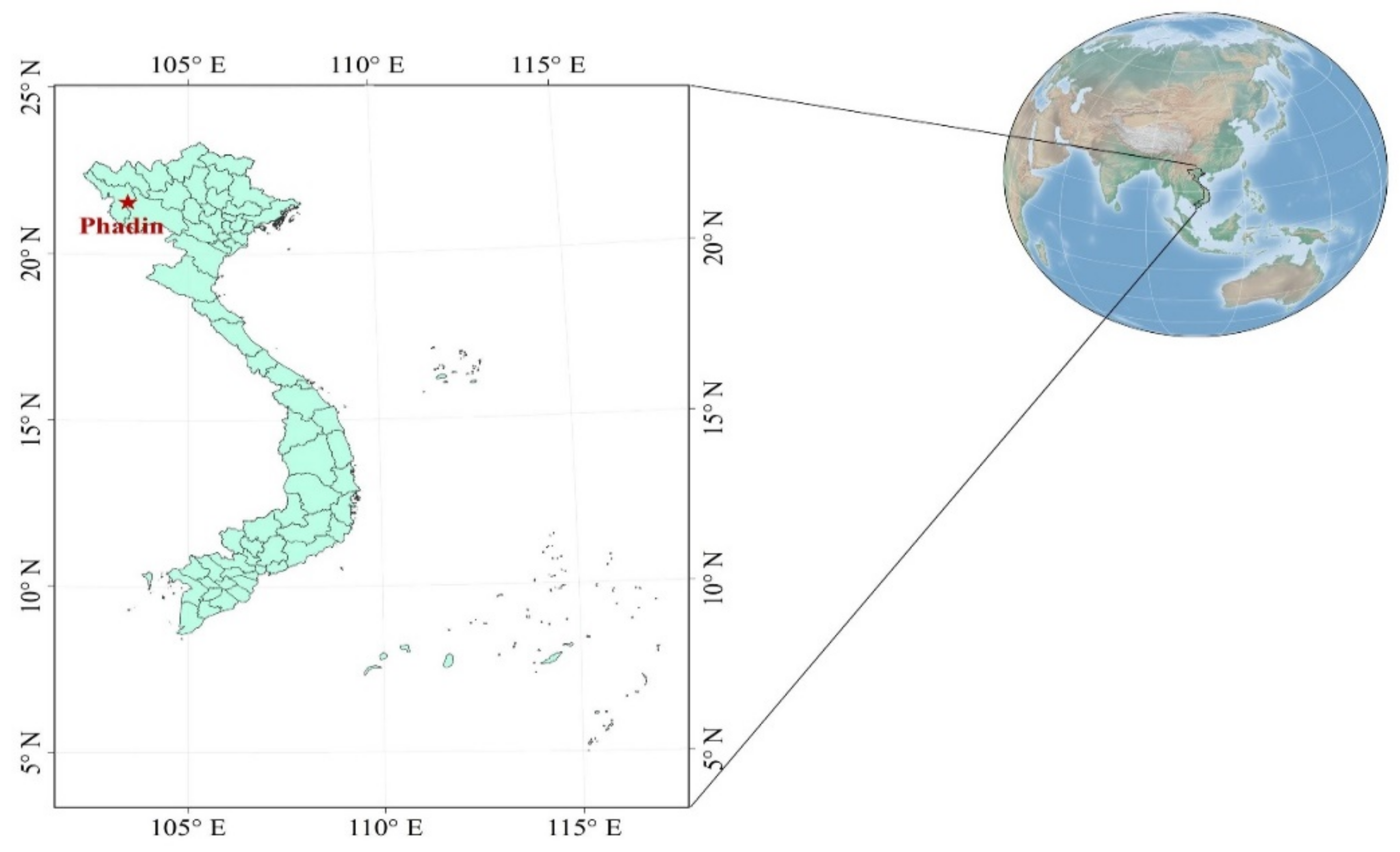
In practice, by using t-SNE [33] for visualizing memory data at every timestamp, the authors in [32] noticed that the memory states are not distinguished between each other automatically and decoupled spontaneously. Based on the PredRNN, the authors established a new loss function, which is the combination of the standard mean square error loss and the new decoupling loss:
L = L M S E + L d e c o u p l e
in which L M S E is the conventional loss function for the former version PredRNN, and L d e c o u p l e is the novel memory decoupling regularization loss function, which is described as follows:
Δ C t l = W d e c o u p l e i t g t Δ M t l = W d e c o u p l e i t g t L d e c o u p l e = t l c Δ C t l ,   Δ M t l c Δ C t l c · Δ M t l c
where W d e c o u p l e is the parameter of a convolution layer added after the memory cells C t l and M t l at each timestep. By this means, two memory states are separated to train on different aspects of spatiotemporal and temporal information. Further, the new convolution layer is removed in the predicting phase, making the size of the entire model unchanged. That makes a novel version of the PredRNN, PredRNN_v2 [28].

2.2. Study Area

In this study, we utilized a radar echo dataset, which was retrieved from the Phadin weather radar station, located in Dien Bien province, Vietnam. The Phadin station, located at 21.58° N and 103.52° S, is under the direct management of the Northwest Aero-Meteorological Observatory and has the primary task of providing short-term forecast information on meteorology and climate for the provinces in this region. Officially launched and operating since March 2019, this is a doppler weather radar station and operates in dual-polarization mode. This means that it is capable of transmitting and receiving pulses of radio waves in both vertical and horizontal directions (Figure 1).
As a result, it can provide super-high-resolution weather observations and cover a large area with an effective scanning radius of up to 300 km. For the issue of precipitation nowcasting based on weather radar, the collected data here is understood as the composite reflectivity images of radio pulses, in which, these images are grayscale images, and each image represents a transmission and reception of a weather radar signal. With an area coverage of 300 km × 300 km (equivalent to the effective range of radar), these reflectivity images have a spatial resolution of 150 × 150 pixels and a corresponding temporal resolution of 10 min. A total of 2429 weather radar composite reflectivity images were collected during rainfall events that took place between June and July 2020 (in the rainy season of Vietnam). Several weather radar images are illustrated in Figure 2.

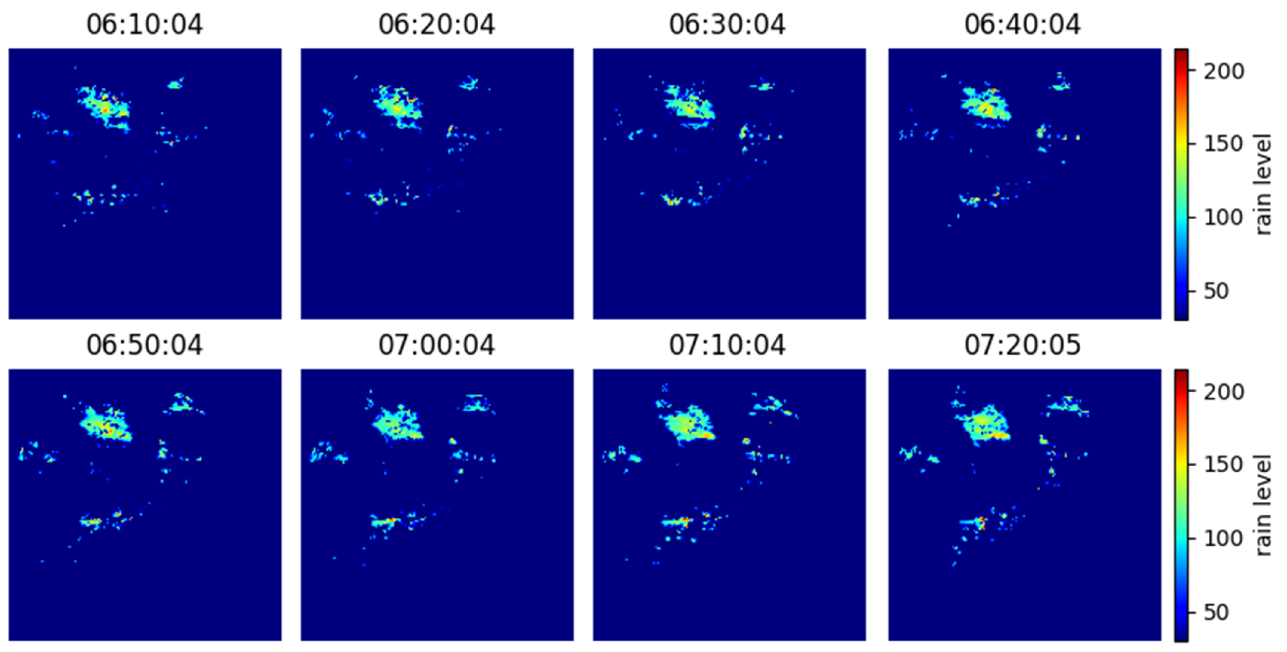
2.3. Data Preparation

In neural networks, the dataset split ratio depends mainly on the data characteristics, the total number of collected samples, and the actual model being trained. The single hold-out method [34] is one of the simplest data resampling strategies that will be applied to our training strategies. In order to train our model effectively and to produce excellent model performance, we randomly divide our gathered dataset into separated three parts: training, validation, and testing set with a ratio of 80:10:10, respectively. This means that in 2429 images of the dataset, the training, validation, and testing set will contain precisely 1947, 242, and 242 images, respectively, to the above ratio. In particular:
  • Training set: The weights and biases of the model will be trained and updated on the samples of the set until reaching convergence.
  • Validation set: An unbiased evaluation will be calculated to see how fit the model is on the training set. This set helps to improve the model performance by fine-tuning the model,
  • Testing set: This set informs us about the final accuracy of the model after completing the training phase.
The details of how the dataset was divided are presented in Table 1, as follows:
In order to make the images as inputs for our model, we stack all images into one array and take the continuous sliding window of the stack sequentially until the index reaches the end. For each consecutive part, we define a number of frames of the head as input and the remainder as output in which a number of timesteps exist in the past. For example, we slide the consecutive image in the array with 10 frames wider per window: 5 for the input and 5 for the output.

2.4. Evaluation Criteria

In the context of computer vision, the mean absolute error (MAE) [35], which is referred to as L 1 loss function in some particular problems, is interpreted as a measure of the difference between every pixel of the predicted image and the ground truth (true value) of that image. Mathematically, the MAE score takes total absolute errors in the entire testing dataset that will be divided by the number of observations. The MAE measure is described in Formula (5) below, where y i ^ and y i are the i th predicted images and the i th ground truth in the testing set, respectively, and the subtraction operation is an element-wise operation:
M A E = 1 n i = 1 n y i ^ y i
Another measure that also has a significant impact on assessing the performance of the model is the structural similarity index measure (SSIM) [36]. The SSIM index calculates the image quality degradation after some processing phase, especially propagating through the deep learning model. Formula (6) below explains the SSIM measure mathematically:
S S I M y , y ^ = 2 μ y μ y ^ + c 1 2 σ y y ^ + c 2 μ y 2 + μ y ^ 2 + c 1 σ y 2 + σ y ^ 2 + c 2
In Formula (6), μ and σ are respectively the average and variance of the label y and the prediction y ^ , and σ y y ^ is the covariance of two images ( y and y ^ ). Furthermore, c 1 and c 2 are two variables responsible for stabilizing the division and are presented as follows:
c 1 = k 1 L 2 c 2 = k 2 L 2
where k 1 = 0.01 and k 2 = 0.03 are set by default, and L = 2 # b i t s   p e r   p i x e l 1 is the dynamic range of the pixel value of the image.
Third, we also use the critical success index (CSI) [37], which is considered as the threat score to evaluate how well our model performs compared to former models. Suppose that we use the four quantities of the confusion matrix [38], which is described in Table 2.
In Table 2, true positive (TP) is the number of ground-truth-positive pixels (Rain) that were correctly predicted. False positive (FP) corresponds to the number of ground-truth-negative pixels (No Rain) that were predicted incorrectly. False negative (FN) is the number of ground-truth-positive pixels that were not predicted. True negative (TN) corresponds to the number of ground-truth-negative pixels that were correctly predicted as negative. The CSI score is shown as follows in Equation (8):
C S I = T P T P + F P + F N
In the current paper, since our modification focuses on reducing the processing time of the deep learning models, the training and testing time is also evaluated as a crucial factor for assessing the performance of models. The last criterion that we include in the evaluation phase is the multiply-accumulate operations (MACs), i.e., a MAC has one multiply operation and one add operation. We clearly detail the model implementation and evaluation results in Section 4.

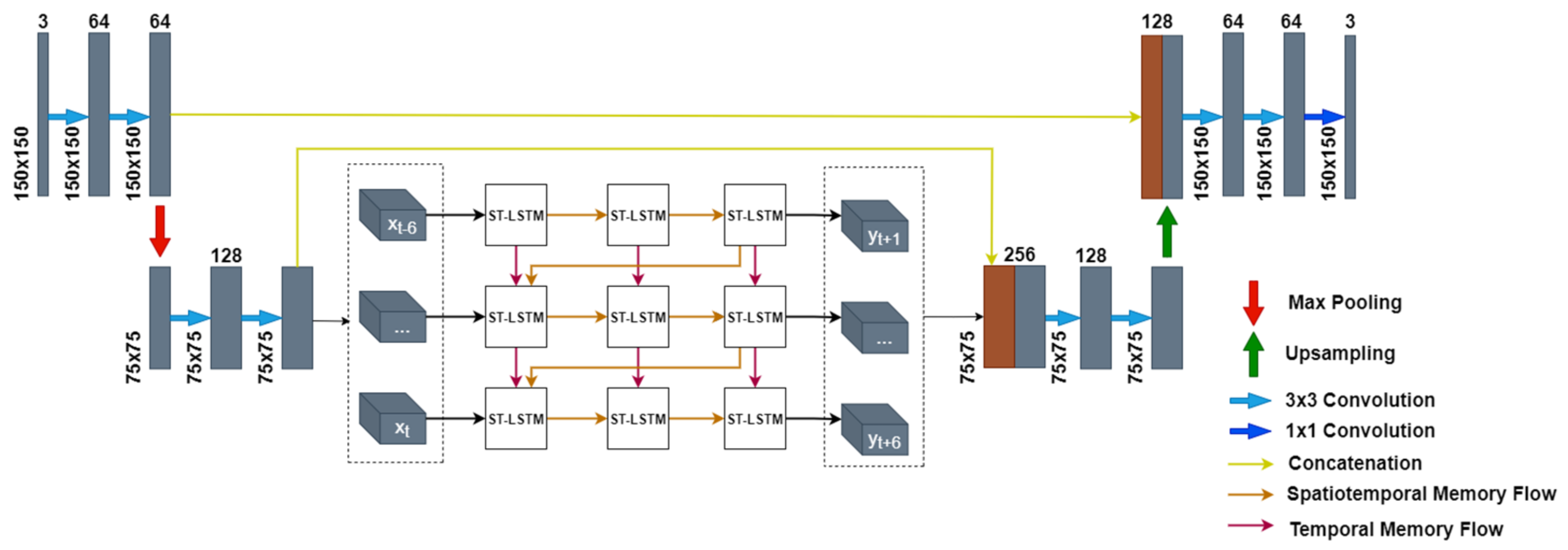
3. Proposed RainPredRNN

In this article, by utilizing the strength of the PredRNN_v2 model, we propose the new modified model, RainPredRNN, which can be fitted into the problems of processing time-series radar images for predicting images in the following time step. Our model uses the contracting-expansive path of the UNet model as the encoder and decoder paths before and after forwarding input to the ST-LSTM layers, which will reduce the huge number of operations required to be calculated.

3.1. Benefit of the Encoder–Decoder Path

Since the robustness of the UNet model has been verified in various domains over the years from its first publication [29], we borrow the UNet-based architecture in order to make our modifications. Thus, the proposed model will benefit from the abilities of the contracting-expansive path and concatenation technique.
Encoder path: Two 3 × 3 convolution layers are repeatedly included to capture the context of original images, and each layer is followed by a rectified linear unit (ReLU) for making the model nonlinear and batch normalization (regularization). In order to reduce the spatial dimensions, a pooling layer, which is a max-pooling layer, is applied right after these convolution layers. After each of the above operations, the original inputs are cut in half the spatial dimensions and double the number of feature channels to produce high-level feature maps.
Decoder path: First, the model must upsample the feature map produced by the encoder path to return to its original shape gradually. Secondly, after each upsampling operator, the number of feature channels will be cut in half by a 2 × 2 transpose convolution layer. In addition, a concatenation technique will be used from the corresponding feature map in the encoder path in order to avoid vanishing the gradients when training. Third, two 3 × 3 convolution layers with ReLU and batch normalization operations are applied. At the final layer, a 1 × 1 convolution layer is used to map every pixel to the desired number of classes.

3.2. Unified RainPredRNN

In order to take advantage of the UNet model, we will borrow the key characteristics of its architecture: contracting-expansive path and concatenation technique. Firstly, every original image is propagated through the encoder path with one max-pooling layer coming between four 3 × 3 convolution layers. By doing this, the high-level valuable contexts of the inputs will be captured and stored in the feature maps before processing by the spatiotemporal LSTM layers (ST-LSTM). Since various image resizing algorithms cause the loss of image information considerably and transform images improperly, the encoder path keeps as much context as possible and still reduces the spatial dimension of original images.
Since ST-LSTM is designed with many gates and a huge number of floating-point operations, the larger the inputs come in, the more calculations are operated. After the encoding path, the original inputs are halved by the width and height and have more spatial information. Thus, the computation time of ST-LSTM will be reduced significantly in both the forward and backward propagation strategies. The visualization of our modification is shown in Figure 3 as follows:
The expansive path was added right after ST-LSTM layers, the outputs of the layers were taken as the inputs. At this time, the skip-connection technique was applied to take the cropped of the corresponding feature map in the encoding path to obtain more information and avoid the gradient vanishing problem. By using one upsampling layer, we obtained the original spatial dimension of the original images. We noticed that our modification remarkably reduced training and testing time, while the model still produced the same evaluated scores as the former version. We detail our experimental results in Section 4.

3.3. Implementation

In this subsection, to be able to predict six next frames (1 h in advance), all models are set up in a proper manner. In practice, after conducting various experiments, we empirically chose the best-fit hyperparameters for our model and resources.
To clarify our implementation in detail, we describe our hyperparameters, which were practically most suitable with our dataset. Our modification model RainPredRNN comprises the critical characteristics of the UNet architecture presented in Section 3.1, in which the kernel size of convolution layers is set to 3 × 3, and both stride and padding were equal to 1. With this choice, our model captures the objects (rain) of our dataset because the pixels move slowly.
In the main body of the model, we put two consecutive ST-LSTM layers together, which were set up with 64 hidden states each and a 3 × 3 filter of the inside convolution layers. Because the size of our input image is quite small, the number of stacked ST-LSTM layers with the hidden states was kept at a moderate size. In addition, the total input length was fixed to 12 frames, with the first six consecutive images for input and the last six ones for ground truth. Thus, to compare the performance of all models, we trained each one in 100 epochs, in which the batch size was set equal to 4, and the learning rate was set equal to 0.001 during the training phase. All the models were evaluated with the above-mentioned criteria. The results are shown in the following section, where, in particular, the three baseline models (PredRNN, PredRNN_v2, and RainPredRNN) are implemented and compared. Finally, all hyperparameters were chosen based on the knowledge about the dataset and by different scenarios practically.
For implementing conveniently, we used the state-of-the-art machine learning PyTorch library written in the Python programming language. These software libraries are free open-source software for communities who want to develop and build machine learning models in research and production. In addition, to visualize the model’s results, we also imported and implemented the Matplotlib library. All algorithms and models used in the paper are listed in the Appendix A.

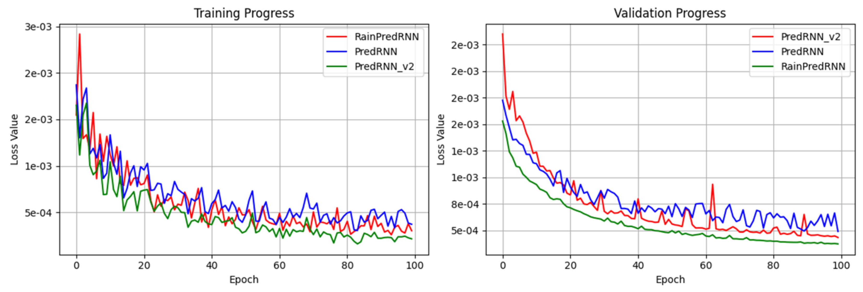
4. Results and Discussion

To conveniently implement and debug our source code properly, we prepared a single powerful workstation running on the Windows 10 64-bit operating system. The machine was equipped with one 12 Gb GPU card, GeForce RTX 2080 Ti. In order to run the proposed deep learning model RainPredRNN on the GPU, we also installed the compatible version 10.1 of the CUDA driver, which can be integrated with the NVIDIA card.
In Figure 4, we observed that the models all converged to the same point as training and validation progressed, approximately 2.5 e 4 and 4 e 4 of the loss value, respectively. The detail of evaluation scores is listed in Table 3, in which MAE, CSI, and SSIM are estimated in the test set. From the table, it can be seen that the SSIM measure of all models is not significantly different (around 0.94), which means that the quality of the images is not degraded after propagating.
It is considered that the model RainPredRNN takes only below 30% of the training time of PredRNN and PredRNN_V2. We can benefit from this point. It will have significant meaning in the future if new training data arrive, and we want to produce a new version. The MAC value of RainPredRNN is one second compared to the others, at about 54 billion, so we can conclude that our modification remarkably reduced the number of operations that need to be processed when training and testing. In addition, our model still has great performance compared to former models. From the result, the models certainly produce the predicted image with high quality and resolution.
Figure 5 shows the input and the ground truth that we used to test our model with the former versions. A prediction example of three models is depicted in Figure 6 and Figure 7. The quality of our model tends to have a higher resolution and be more precise than that of the models PredRNN and PredRNN_v2.
From these results, we can infer that the family of the PredRNN model is suitable for the problem of precipitation nowcasting, and our proposed model can help reduce training and testing significantly and also produces high-quality future images in a short time.

5. Conclusions

In this paper, we proposed a new deep learning model, RainPredRNN, for precipitation nowcasting with weather radar echo images. This model is a combination of UNet and PredRNN_v2 with the purpose of reducing training and testing time while preserving the complex spatial features of radar data. RainPredRNN manages both spatiotemporal and temporal information of time-series images. Additionally, the contracting and expanding paths of UNet have a vital role in reducing the size of inputs, while it still captures the high-level features of original images. The experiments on real data from the Phadin weather radar station, located in Dien Bien province, Vietnam, have clearly affirmed that RainPredRNN reduces training and testing significantly and also produces high-quality future images in a short time. The proposed approach has produced comparable results in which the training time is equal to less than 30% training time and 50% MAC value of the former versions.
However, some limitations of the proposed model remain, such as the validation measures are not outstanding compared to the former measures. We retained the core ST-LSTM layer as a building block, so the layer needs to be modified down the road. In the future, we hope that we will also make further improvements to the accuracy of the model for precipitation nowcasting.

Author Contributions

Conceptualization, methodology, software: D.N.T., T.M.T., L.H.S.; data curation, writing—original draft preparation: D.N.T., T.M.T., X.-H.L.; visualization, investigation: T.K.C., P.V.H.; software, validation: D.N.T., T.M.T.; supervision: L.H.S., V.C.G.; writing—reviewing and editing: N.T.T., V.C.G., L.H.S. All authors have read and agreed to the published version of the manuscript.

Funding

This research was funded by the Thuyloi University Foundation for Science and Technology.

Acknowledgments

The authors would like to acknowledge the editors and reviewers who provided valuable comments and suggestions that improved the quality of the manuscript.

Conflicts of Interest

The authors declare that they do not have any conflict of interests. This research does not involve any human or animal participation. All authors have checked and agreed with the submission.

Appendix A

List of all algorithms and models used in the paper:
  • Adam is the learning algorithm that is used in the training phase to seek the convergence point of the model. The parameters of the model are modified until the model converges.
  • Convolutional LSTM is the general version of LSTM that is designed to tackle the problem of processing image inputs. By replacing the multiply operator with the convolution operator of spatial structure information, the model successfully encodes the spatial structure information of input.
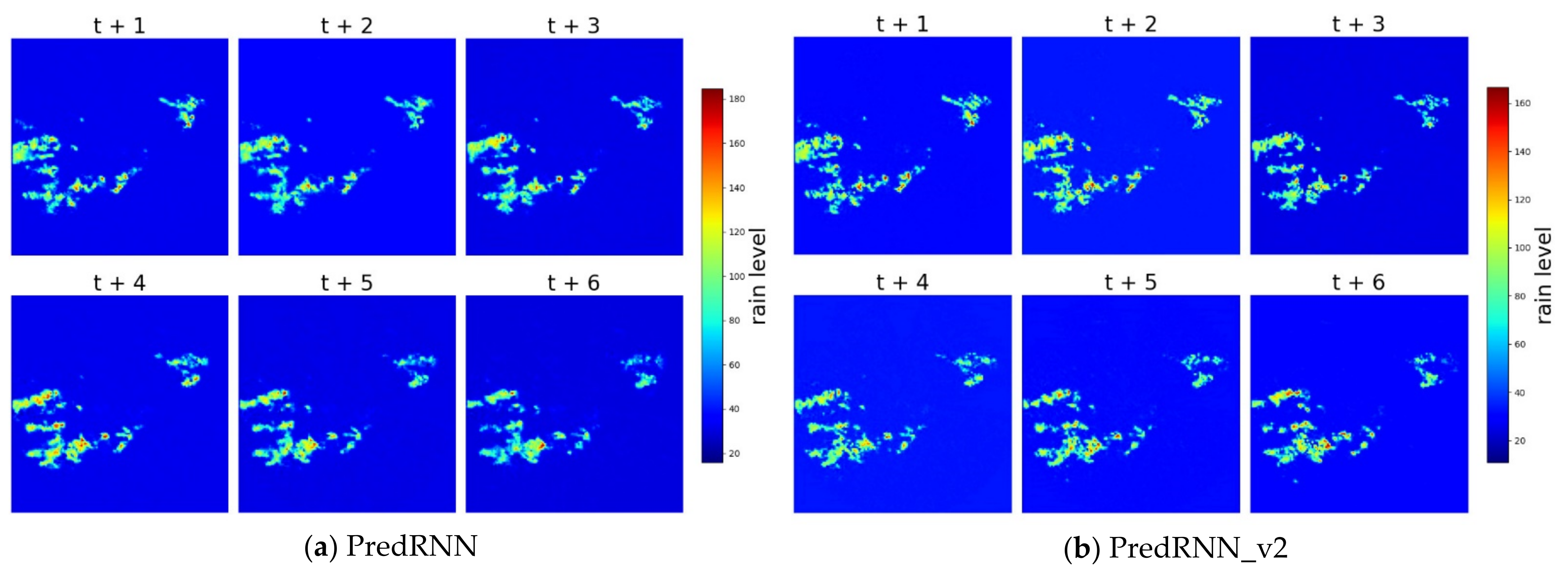
  • PredRNN combines the spatiotemporal LSTM (ST-LSTM) as the building block with the memory flow technique. The ST-LSTM introduces improvements to the memory cells, which contain the information of the flow (the memory flow technique) in both horizontal and vertical directions.
  • PredRNN_v2 introduces the new component of the final loss function. This improvement trains the model more effectively and successfully, but the overall size of the model remains.
  • RainPredRNN is the proposed model, which is a combination of the strength of the PredRNN_v2 model and the UNet model. The model borrows the contracting and expansive path of the UNet model for processing input to reduce the computational operators of the overall model. From that, the proposed model produces satisfactory results in a short time.

References

  1. Wapler, K.; de Coning, E.; Buzzi, M. Nowcasting. In Reference Module in Earth Systems and Environmental Sciences; Elsevier: Amsterdam, The Netherlands, 2019. [Google Scholar] [CrossRef]
  2. CRED. Natural Disasters; Centre for Research on the Epidemiology of Disasters (CRED): Brussels, Belgium, 2019; Available online: https://www.cred.be/sites/default/files/CREDNaturalDisaster2018.pdf (accessed on 10 October 2021).
  3. Keay, K.; Simmonds, I. Road accidents and rainfall in a large Australian city. Accid. Anal. Prev. 2006, 38, 445–454. [Google Scholar] [CrossRef]
  4. Chung, E.; Ohtani, O.; Warita, H.; Kuwahara, M.; Morita, H. Effect of rain on travel demand and traffic accidents. In Proceedings of the IEEE Intelligent Transportation Systems, Vienna, Austria, 16 September 2005; pp. 1080–1083. [Google Scholar]
  5. Sun, Q.; Miao, C.; Duan, Q.; Ashouri, H.; Sorooshian, S.; Hsu, K.-L. A Review of Global Precipitation Data Sets: Data Sources, Estimation, and Intercomparisons. Rev. Geophys. 2018, 56, 79–107. [Google Scholar] [CrossRef] [Green Version]
  6. LeCun, Y.; Bengio, Y.; Hinton, G. Deep learning. Nature 2015, 521, 436–444. [Google Scholar] [CrossRef] [PubMed]
  7. Sit, M.A.; Demiray, B.Z.; Xiang, Z.; Ewing, G.; Sermet, Y.; Demir, I. A Comprehensive Review of Deep Learning Applications in Hydrology and Water Resources. Water Sci. Technol. 2020, 82, 2635–2670. [Google Scholar] [CrossRef] [PubMed]
  8. Gao, Z.; Shi, X.; Wang, H.; Yeung, D.; Woo, W.; Wong, W. Deep Learning and the Weather Forecasting Problem: Precipitation Nowcasting. In Deep Learning for the Earth Sciences: A Comprehensive Approach to Remote Sensing, Climate Science, and Geosciences; John Wiley & Sons, Ltd.: Hoboken, NJ, USA, 2021; pp. 218–239. [Google Scholar] [CrossRef]
  9. Simonyan, K.; Zisserman, A. Very Deep Convolutional Networks for Large-Scale Image Recognition. arXiv 2014, arXiv:1409.1556. [Google Scholar]
  10. Zhao, Z.-Q.; Zheng, P.; Xu, S.-T.; Wu, X. Object Detection With Deep Learning: A Review. IEEE Trans. Neural Netw. Learn. Syst. 2019, 30, 3212–3232. [Google Scholar] [CrossRef] [Green Version]
  11. Le, X.H.; Lee, G.; Jung, K.; An, H.-U.; Lee, S.; Jung, Y. Application of Convolutional Neural Network for Spatiotemporal Bias Correction of Daily Satellite-Based Precipitation. Remote Sens. 2020, 12, 2731. [Google Scholar] [CrossRef]
  12. Ayzel, G.; Scheffer, T.; Heistermann, M. RainNet v1.0: A convolutional neural network for radar-based precipitation nowcasting. Geosci. Model Dev. 2020, 13, 2631–2644. [Google Scholar] [CrossRef]
  13. Khiali, L.; Ienco, D.; Teisseire, M. Object-oriented satellite image time series analysis using a graph-based representation. Ecol. Inform. 2018, 43, 52–64. [Google Scholar] [CrossRef] [Green Version]
  14. Fahim, S.R.; Sarker, Y.; Sarker, S.K.; Sheikh, R.I.; Das, S.K. Self attention convolutional neural network with time series imaging based feature extraction for transmission line fault detection and classification. Electr. Power Syst. Res. 2020, 187, 106437. [Google Scholar] [CrossRef]
  15. Li, X.; Kang, Y.; Li, F. Forecasting with time series imaging. Expert Syst. Appl. 2020, 160, 113680. [Google Scholar] [CrossRef]
  16. Ravuri, S.; Lenc, K.; Willson, M.; Kangin, D.; Lam, R.; Mirowski, P.; Fitzsimons, M.; Athanassiadou, M.; Kashem, S.; Madge, S.; et al. Skilful precipitation nowcasting using deep generative models of radar. Nature 2021, 597, 672–677. [Google Scholar] [CrossRef] [PubMed]
  17. Li, D.; Liu, Y.; Chen, C. MSDM v1.0: A machine learning model for precipitation nowcasting over eastern China using multisource data. Geosci. Model Dev. 2021, 14, 4019–4034. [Google Scholar] [CrossRef]
  18. Chen, L.; Cao, Y.; Ma, L.; Zhang, J. A Deep Learning-Based Methodology for Precipitation Nowcasting with Radar. Earth Space Sci. 2020, 7, e2019EA000812. [Google Scholar] [CrossRef] [Green Version]
  19. Agrawal, S.; Barrington, L.; Bromberg, C.; Burge, J.; Gazen, C.; Hickey, J. Machine Learning for Precipitation Nowcasting from Radar Images. arXiv 2019, arXiv:1912.12132. [Google Scholar]
  20. Fernández, J.G.; Mehrkanoon, S. Broad-UNet: Multi-scale feature learning for nowcasting tasks. Neural Netw. 2021, 144, 419–427. [Google Scholar] [CrossRef]
  21. Ionescu, V.-S.; Czibula, G.; Mihuleţ, E. DeePS at: A deep learning model for prediction of satellite images for nowcasting purposes. Procedia Comput. Sci. 2021, 192, 622–631. [Google Scholar] [CrossRef]
  22. Zhang, L.; Huang, Z.; Liu, W.; Guo, Z.; Zhang, Z. Weather radar echo prediction method based on convolution neural network and Long Short-Term memory networks for sustainable e-agriculture. J. Clean. Prod. 2021, 298, 126776. [Google Scholar] [CrossRef]
  23. Trebing, K.; Staǹczyk, T.; Mehrkanoon, S. SmaAt-UNet: Precipitation nowcasting using a small attention-UNet architecture. Pattern Recognit. Lett. 2021, 145, 178–186. [Google Scholar] [CrossRef]
  24. Le, X.H.; Ho, H.V.; Lee, G.; Jung, S. Application of Long Short-Term Memory (LSTM) Neural Network for Flood Forecasting. Water 2019, 11, 1387. [Google Scholar] [CrossRef] [Green Version]
  25. Le, X.H.; Nguyen, D.H.; Jung, S.; Yeon, M.; Lee, G. Comparison of Deep Learning Techniques for River Streamflow Forecasting. IEEE Access 2021, 9, 71805–71820. [Google Scholar] [CrossRef]
  26. Kreklow, J.; Tetzlaff, B.; Burkhard, B.; Kuhnt, G. Radar-Based Precipitation Climatology in Germany—Developments, Uncertainties and Potentials. Atmosphere 2020, 11, 217. [Google Scholar] [CrossRef] [Green Version]
  27. Otsuka, S.; Kotsuki, S.; Ohhigashi, M.; Miyoshi, T. GSMaP RIKEN Nowcast: Global Precipitation Nowcasting with Data Assimilation. J. Meteorol. Soc. Jpn. 2019, 97, 1099–1117. [Google Scholar] [CrossRef] [Green Version]
  28. Wang, Y.; Wu, H.; Zhang, J.; Gao, Z.; Wang, J.; Yu, P.; Long, M. PredRNN: A Recurrent Neural Network for Spatiotemporal Predictive Learning. arXiv 2021, arXiv:2103.09504. [Google Scholar]
  29. Ronneberger, O.; Fischer, P.; Brox, T. U-Net: Convolutional Networks for Biomedical Image Segmentation. arXiv 2015, arXiv:1505.04597. [Google Scholar]
  30. Cho, K.; van Merriënboer, B.; Gulcehre, C.; Bahdanau, D.; Bougares, F.; Schwenk, H.; Bengio, Y. Learning phrase representations using RNN encoder-decoder for statistical machine translation. arXiv 2014, arXiv:1406.1078. [Google Scholar]
  31. Shi, X.; Chen, Z.; Wang, H.; Yeung, D.-Y.; Wong, W.-K.; Woo, W.-C. Convolutional LSTM Network: A Machine Learning Approach for Precipitation Nowcasting. arXiv 2015, arXiv:1506.04214. [Google Scholar]
  32. Wang, Y.; Long, M.; Wang, J.; Gao, Z.; Yu, P. PredRNN: Recurrent Neural Networks for Predictive Learning using Spatio-temporal LSTMs. In Advances in Neural Information Processing Systems; Guyon, I., Luxburg, U.V., Bengio, S., Wallach, H., Fergus, R., Vishwanathan, S., Garnett, R., Eds.; Curran Associates, Inc.: Red Hook, NY, USA, 2017; Volume 30. [Google Scholar]
  33. Maaten, L.; Hinton, G. Visualizing Data using t-SNE. J. Mach. Learn. Res. 2008, 9, 2579–2605. [Google Scholar]
  34. Berrar, D. Cross-Validation. In Encyclopedia of Bioinformatics and Computational Biology; Elsevier: Amsterdam, The Netherlands, 2019. [Google Scholar]
  35. Chai, T.; Draxler, R.R. Root mean square error (RMSE) or mean absolute error (MAE)?—Arguments against avoiding RMSE in the literature. Geosci. Model Dev. 2014, 7, 1247–1250. [Google Scholar] [CrossRef] [Green Version]
  36. Wang, Z.; Bovik, A.; Sheikh, H.; Simoncelli, E. Image quality assessment: From error visibility to structural similarity. IEEE Trans. Image Process 2004, 13, 600–612. [Google Scholar] [CrossRef] [Green Version]
  37. Schaefer, J. The Critical Success Index as an Indicator of Warning Skill. Weather. Forecast. 1990, 5, 570–575. [Google Scholar] [CrossRef] [Green Version]
  38. Townsend, J. Theoretical analysis of an alphabetic confusion matrix. Percept. Psychophys. 1971, 9, 40–50. [Google Scholar] [CrossRef]
Figure 1. Geographical area of the region of study.
Axioms 11 00107 g001
Figure 2. Samples of radar reflectivity images were recorded in the period between 6:10 a.m. and 7:20 a.m. on 23 June 2020. The pixels with high value (white) denote raining areas. In contrast, the low-value pixels are not raining areas.
Axioms 11 00107 g002
Figure 3. Unified RainPredRNN model. The boxes with the text “ST-LSTM” denote the conventional spatiotemporal LSTM, the gray boxes represent images in different processing levels of the model, and the brown boxes are the copy of cropped feature maps. While the encoding path has a role in reducing the spatial dimension of inputs for lightweight computation of the stacked ST-LSTM, the decoding path processes the output of the stacked ST-LSTM to recover back to the original size of the output.
Axioms 11 00107 g003
Figure 4. Training and validation loss of models.
Axioms 11 00107 g004
Figure 5. Consecutive image input and ground truth for comparison: (a) input; (b) ground truth.
Axioms 11 00107 g005
Figure 6. Predicted image of compared models: (a) six next predicted frames of model PredRNN; (b) next six predicted frames of PredRNN_v2.
Axioms 11 00107 g006
Figure 7. Six consecutive frames output of RainPredRNN model.
Axioms 11 00107 g007
Table 1. Quantity and size of each dataset.
DatasetQuantitySize
Training Set1947150 × 150
Validation Set242150 × 150
Testing Set242150 × 150
Table 2. Confusion matrix.
Ground Truth
RainNo Rain
PredictedRainTPFP
No RainFNTN
Table 3. Evaluation scores of our modification model with others.
ModelMAECSISSIMTraining Time (hour)MACs(G)
PredRNN0.45350.94550.939715.1101.469
PredRNN_v20.41570.94200.943015.53103.885
RainPredRNN0.43010.95900.94124.4654.705
Publisher’s Note: MDPI stays neutral with regard to jurisdictional claims in published maps and institutional affiliations.

