Reliability-Based Design Optimization of Structures Considering Uncertainties of Earthquakes Based on Efficient Gaussian Process Regression Metamodeling

Abstract

The complexity of earthquakes and the nonlinearity of structures tend to increase the calculation cost of reliability-based design optimization (RBDO). To reduce computational burden and to effectively consider the uncertainties of ground motions and structural parameters, an efficient RBDO method for structures under stochastic earthquakes based on adaptive Gaussian process regression (GPR) metamodeling is proposed in this study. In this method, the uncertainties of ground motions are described by the record-to-record variation and the randomness of intensity measure (IM). A GPR model is constructed to obtain the approximations of the engineering demand parameter (EDP), and an active learning (AL) strategy is presented to adaptively update the design of experiments (DoE) of this metamodel. Based on the reliability of design variables calculated by Monte Carlo simulation (MCS), an optimal solution can be obtained by an efficient global optimization (EGO) algorithm. To validate the effectiveness and efficiency of the developed method, it is applied to the optimization problems of a steel frame and a reinforced concrete frame and compared with the existing methods. The results show that this method can provide accurate reliability information for seismic design and can deal with the problems of minimizing costs under the probabilistic constraint and problems of improving the seismic reliability under limited costs.

1. Introduction

Due to environmental changes, manual operation, manufacturing process, and other factors in the construction or use of engineering structures, there are usually uncertainties in component size, material properties, and external loads. According to the guidelines [1], the structure under seismic load should reach performance levels related to a set of specified reliability criteria during the design service life. Incorporating RBDO into seismic design can provide an ideal tool for designers to realize this design principle [2,3]. Compared with deterministic optimization, RBDO can take the uncertainties of structural performance into account and can achieve a balance between the structural reliability and costs [4].

Reliability-based seismic optimization is characterized by considering the uncertainties of earthquakes. Seismic load is a complex external excitation. Recent studies have been devoted to the application of RBDO in structural seismic design. Mishra et al. [5] studied the influence of parameter uncertainty on the optimization results of base-isolated structures subjected to random earthquakes, in which the structural response is obtained by the framework of random vibration analysis. Zou et al. [4] proposed an RBDO procedure for reinforced concrete buildings with fiber-reinforced polymer composites, taking the inter-storey displacement of structures as the performance parameter. Ni et al. [2] applied the first-order reliability method (FORM) and Kriging model to RBDO of nonlinear steel frames and reinforced concrete frames, where the uncertainties of structural parameters are considered. In the research studies of Refs. [2,4], structural response is calculated by the Pushover method, where uncertainties associated with the frequency content of ground motions are difficult to be taken into account. Hadidi et al. [6] optimized semi-rigidly connected base-isolated buildings subjected to near-fault stochastic earthquakes. Yazdani et al. [3] developed an optimization method for RBDO problems of reinforced concrete structures considering soil-structure interaction effects, in which the MCS method was adopted to calculate the reliability and the support vector machine (SVM) approach was employed to evaluate the structural response. Peng et al. [7] proposed an RBDO framework for base isolation systems, which used sensitivity analysis to identify critical design parameters and employed probability density evolution method to analyze the reliability of structures. In the studies of Refs. [3,6,7], the artificial records generated by ground motion models rather than natural records are required for dynamic analysis.

As reliability needs to be evaluated in optimization, the number of calls to structural analysis in RBDO is far more than that in deterministic design optimization. Furthermore, the complexity of earthquakes and nonlinearity of structures further increase computational burden. In addition to the randomness of IM, there is also uncertainty in the frequency contents and other dynamic characteristics of seismic ground motions, which is called record-to-record variation [8]. The reliability problems considering the uncertainties of earthquakes and structural parameters can be addressed by probabilistic evaluation methods combining MCS with nonlinear time history analysis (NLTHA) [9,10]. However, NLTHA for response calculation is very time consuming, and calling for structural analysis repeatedly will generate huge computational costs. In order to improve calculation efficiency, metamodel (also known as surrogate model) approaches are introduced into the probabilistic evaluation of seismic performance, such as the response surface methodology (RSM) [11], artificial neural network (ANN) [12], SVM [13], and radial basis function [14]. The dual RSM-based seismic reliability analysis (D-RSM-SRA) approach proposed by Towashiraporn [15] is a commonly used seismic risk assessment method. In this method, the dual RSM framework where the EDP is assumed to follow a certain random distribution is adopted to deal with the record-to-record variation, which overcomes the difficulty of handling the input of high-dimensional seismic time history in metamodeling. Two RSM models are constructed to estimate the mean and standard deviation of the stochastic response, respectively, and the response approximation obtained by the models is used as a substitute for the real response in MCS. D-RSM-SRA has been widely used in probability analysis of seismic performance of various structures, such as track-on steel-plate-girder bridge [16], base-isolated liquid storage tank [17], bridge pier [18], nuclear power plant [11], reinforced concrete bridge [19], and base-isolated frame [20]. Datta et al. [21] applied the dual RSM framework to reliability-based optimization, and their developed method can efficiently solve the optimization problem considering record-to-record variation. However, the DoE for building dual RSM models is often obtained by one-shot sampling, which may lead to a difficulty in predetermining the number of samples for different structures [22]. In addition, it is difficult to pay more attention to the positions that have a key influence on calculation results in the sampling space by one-shot sampling. Obviously, these factors will affect computational efficiency and result accuracy.

For general RBDO problems, in order to reasonably choose DoE, researchers applied adaptive sampling in metamodeling and proposed a number of RBDO methods based on adaptive metamodeling, such as sequential maximum expected improvement sampling strategy based on the performance measurement analysis [23], RBDO approach using efficient global reliability analysis and EGO (EGO-EGRA) [24], local adaptive sampling [25], active learning method with Kriging and chaotic single loop [26], and dismantled method based on quantile [27]. Such approaches first build the initial metamodel with a small number of experiments and then add new samples to the DoE until the model has sufficient accuracy. They do not require the metamodel to be globally accurate, but the accuracy at locations that have a great influence on the optimization results in terms of the complexity of the problem is improved, thus reducing the number of samples for metamodeling. However, in these methods, the value of each performance function or structural response is estimated by one metamodel, and the metamodel needs to have the ability to evaluate the error of estimation. Therefore, they cannot be directly used to improve the accuracy of dual RSM metamodels.

In order to reduce calculation costs and to effectively consider the uncertainties of earthquakes in optimization, in this research, an RBDO approach for structures subjected to seismic load based on adaptive GPR metamodeling is proposed. In this method, the same assumption of seismic demand as in the dual RSM framework is adopted to deal with the record-to-record variation, but the number of metamodels corresponding to each performance function is reduced to one. An AL sampling strategy is given to improve the EGO-EGRA algorithm, and it is used in adaptive modeling of the EDP to search for an optimal solution. In this paper, the RBDO formulation and EGO-EGRA methods are first reviewed. Then, the details of the proposed RBDO framework of structures subjected to earthquake load are presented. Finally, the proposed method is applied to two illustrative examples—a steel frame and a reinforced concrete frame. The first example is a problem of minimizing the costs under the reliability constraint, and the second example is a problem of improving the seismic reliability under limited costs. The analysis results are compared with those of the MCS and EGO-EGRA methods.

2. RBDO Problem and EGO-EGRA Approach

2.1. RBDO Formulation

A general deterministic optimization problem is to find point d* where the objective function takes the extreme value subjected to the constraints, which can be described [28,29] as follows:

$$\begin{array}{l}\mathrm{Find}: \mathbf{d}\\ \mathrm{Minimize}: f(\mathbf{d})\\ \mathrm{Subject} \mathrm{to}: g_i(\mathbf{d})\le 0 i=1,2,\dots ,I\\ {\mathbf{d}}^{\mathrm{L}}\le \mathbf{d}\le {\mathbf{d}}^{\mathrm{U}}\end{array}$$

(1)

where f(d) is the objective function, g_i(d) ≤ 0 denotes the constraint, I represents the number of constraints, d* is called the optimal solution, and the superscripts ‘L’ and ‘U’ denote the lower and upper bounds of variables, respectively.

A typical RBDO form is to minimize the costs of the structure while meeting the reliability constraints [30], which can be described as follows:

$$\begin{array}{l}\mathrm{Find}: \mathbf{D}=[\mathbf{d},{\mathsf{\mu }}_{\mathbf{Z}}]\\ \mathrm{Minimize}: w(\mathbf{d},{\mathsf{\mu }}_{\mathbf{Z}},{\mathsf{\mu }}_{\mathbf{P}})\\ \mathrm{Subject} \mathrm{to}: \mathrm{Pr}\{G(\mathbf{d},\mathbf{Z},\mathbf{P})\le 0\}\le P_T\\ {\mathbf{d}}^{\mathrm{L}}\le \mathbf{d}\le {\mathbf{d}}^{\mathrm{U}},{\mathsf{\mu }}_{\mathbf{Z}}^{\mathrm{L}}\le {\mathsf{\mu }}_{\mathbf{Z}}\le {\mathsf{\mu }}_{\mathbf{Z}}^{\mathrm{U}}\end{array}$$

(2)

where d represents the vector of deterministic design variable, Z and P denote the vectors of random design variable and random parameter, and their mean values are μ_Z and μ_P, respectively; D represents the vector of design variable; $\mathrm{Pr}\{G(\mathbf{d},\mathbf{Z},\mathbf{P})<0\}$ is the failure probability corresponding to the performance function $G(\mathbf{d},\mathbf{Z},\mathbf{P})$; and P_T denotes the target failure probability of the reliability constraint. If the performance function value is positive, the structure is safe; otherwise, it fails. There can be multiple reliability constraints in an RBDO problem. Another form of RBDO is to optimize structural reliability [24], which can be expressed as follows:

$$\begin{array}{l}\mathrm{Find}: \mathbf{D}=[\mathbf{d},{\mathsf{\mu }}_{\mathbf{Z}}]\\ \mathrm{Minimize}: \mathrm{Pr}\{G(\mathbf{d},\mathbf{Z},\mathbf{P})\le 0\}\\ \mathrm{Subject} \mathrm{to}: h(\mathbf{d},{\mathsf{\mu }}_{\mathbf{Z}},{\mathsf{\mu }}_{\mathbf{P}})\le 0\\ {\mathbf{d}}^{\mathrm{L}}\le \mathbf{d}\le {\mathbf{d}}^{\mathrm{U}},{\mathsf{\mu }}_{\mathbf{Z}}^{\mathrm{L}}\le {\mathsf{\mu }}_{\mathbf{Z}}\le {\mathsf{\mu }}_{\mathbf{Z}}^{\mathrm{U}}\end{array}$$

(3)

where $h(\mathbf{d},{\mathsf{\mu }}_{\mathbf{Z}},{\mathsf{\mu }}_{\mathbf{P}})\le 0$ is the deterministic constraint.

2.2. Efficient Global Optimization

Since the objective and constraint functions need to be called repeatedly in solving the optimization problem, the calculation cost of optimization is very high when the function values are obtained by time-consuming finite element analysis (FEA). To improve the efficiency of deterministic optimization, the predicted values $\widehat{f}(\mathbf{d})$ and ${\widehat{g}}_i(\mathbf{d})$ provided by the metamodels of the objective and constraint functions can be used as substitutes for the true values $f(\mathbf{d})$ and $g_i(\mathbf{d})$. Only a small number of response analyses are required to generate the samples for establishing the metamodels. Then, the optimization problem (1) can be transformed into the following.

$$\begin{array}{l}\mathrm{Find}: \mathbf{d}\\ \mathrm{Minimize}: \widehat{f}(\mathbf{d})\\ \mathrm{Subject} \mathrm{to}: {\widehat{g}}_i(\mathbf{d})\le 0 i=1,2,\dots ,I\\ {\mathbf{d}}^{\mathrm{L}}\le \mathbf{d}\le {\mathbf{d}}^{\mathrm{U}}\end{array}$$

(4)

The EGO method [31] is an optimization algorithm using infill-sampling criterion, which can reduce the accuracy loss of the optimization results caused by metamodels. It adopts Gaussian process (GP) model for metamodeling. In this model, the unknown function value is regarded as a normal distribution variable for which its mean is the prediction and standard deviation is the predicted error. For unconstrained optimization problems, this method selects new samples in terms of the expected improvement (EI) function value. The EI function is defined as follows:

$$EI(\mathbf{d})=\left(f_{\mathrm{best}}-\widehat{f}(\mathbf{d})\right)\Phi \left(\frac{f_{\mathrm{best}}-\widehat{f}(\mathbf{d})}{{\sigma }_{\widehat{f}}(\mathbf{d})}\right)+{\sigma }_{\widehat{f}}(\mathbf{d})\cdot \varphi \left(\frac{f_{\mathrm{best}}-\widehat{f}(\mathbf{d})}{{\sigma }_{\widehat{f}}(\mathbf{d})}\right)$$

(5)

where ${\widehat{\sigma }}_{\widehat{f}}(\mathbf{d})$ is the predicted standard deviation of the objective function $f(\mathbf{d})$, f_best is the current best objective value, and $\Phi (\cdot )$ and $\varphi (\cdot )$ are the probability distribution function and probability density function of the standard normal distribution, respectively. The basic steps of EGO are as follows: (1) select a small number of samples in the design space and calculate their function values; (2) establish the metamodel; (3) search for the point d′ with the maximum EI value; and (4) if the convergence condition EI < 0.01·f_best is satisfied at point d′, stop infill-sampling and take the design point d* corresponding to f_best as the optimal solution of the optimization problem, otherwise add point d′ to the DoE and return to step (2).

If the optimization problem contains constraints, the constrained EI (CEI) function can be used to replace the EI function in the EGO procedure. The CEI function [32] is defined as follows:

$$\begin{array}{ll}CEI(\mathbf{d})& =EI(\mathbf{d})\cdot PoF(\mathbf{d})\hfill \\ & =\left[\left(f_{\mathrm{best}}-\widehat{f}(\mathbf{d})\right)\Phi \left(\frac{f_{\mathrm{best}}-\widehat{f}(\mathbf{d})}{{\sigma }_{\widehat{f}}(\mathbf{d})}\right)+{\sigma }_{\widehat{f}}(\mathbf{d})\cdot \varphi \left(\frac{f_{\mathrm{best}}-\widehat{f}(\mathbf{d})}{{\sigma }_{\widehat{f}}(\mathbf{d})}\right)\right]\cdot {\displaystyle \prod _{i=1}^I\Phi \left(\frac{-{\widehat{g}}_i(\mathbf{d})}{{\sigma }_i(\mathbf{d})}\right)}\hfill \end{array}$$

(6)

where ${\sigma }_i(\mathbf{d})$ represents the predicted standard deviation of the constraint function $g_i(\mathbf{d})$.

2.3. EGO-EGRA Approach

Inspired by EGO, Bichon et al. proposed the efficient global reliability analysis (EGRA) method. By integrating EGRA into EGO, three RBDO methods were proposed, namely EGO-EGRA with separate metamodel, EGO-EGRA with single metamodel, and sequential EGO-EGRA [24]. “EGO-EGRA” in this study refers to EGO-EGRA with a single metamodel, which is the most efficient of the three methods.

In EGO-EGRA, a small number of samples were first selected to establish the initial metamodel of the performance function. The input variable vector x of the metamodel consists of d, Z, and P. Then, in order to obtain new samples that can refine the metamodel at the limit state surface, the global optimization algorithm is used to search the x space for the point ${\mathbf{x}}_{new}$ with the maximum EF function value. The EF function is defined as follows

$$\begin{array}{ll}EF(\mathbf{x})& =\left(\widehat{G}(\mathbf{x})-z\right)\left[2\Phi \left(\frac{z-\widehat{G}(\mathbf{x})}{{\sigma }_{\widehat{G}}(\mathbf{x})}\right)-\Phi \left(\frac{z-\xi -\widehat{G}(\mathbf{x})}{{\sigma }_{\widehat{G}}(\mathbf{x})}\right)-\Phi \left(\frac{z+\xi -\widehat{G}(\mathbf{x})}{{\sigma }_{\widehat{G}}(\mathbf{x})}\right)\right]-\hfill \\ & {\sigma }_{\widehat{G}}(\mathbf{x})\left[2\varphi \left(\frac{z-\widehat{G}(\mathbf{x})}{{\sigma }_{\widehat{G}}(\mathbf{x})}\right)-\varphi \left(\frac{z-\xi -\widehat{G}(\mathbf{x})}{{\sigma }_{\widehat{G}}(\mathbf{x})}\right)-\varphi \left(\frac{z+\xi -\widehat{G}(\mathbf{x})}{{\sigma }_{\widehat{G}}(\mathbf{x})}\right)\right]+\hfill \\ & \xi \left[\Phi \left(\frac{z+\xi -\widehat{G}(\mathbf{x})}{{\sigma }_{\widehat{G}}(\mathbf{x})}\right)-\Phi \left(\frac{z-\xi -\widehat{G}(\mathbf{x})}{{\sigma }_{\widehat{G}}(\mathbf{x})}\right)\right]\hfill \end{array}$$

(7)

where $\widehat{G}$ and ${\sigma }_{\widehat{G}}$ are the prediction and predicted error of performance function G, z is the threshold corresponding to the limit state, and ξ is generally taken as $2{\sigma }_{\widehat{G}}$. The EF value at a point indicates how well the real function value at this point is expected to satisfy equality constraint $G=z$. A point where the prediction is close to z and the predicted error is large has a large EF value [33]. When the value of $EF({\mathbf{x}}_{new})$ is small, the metamodel is considered to be accurate enough and sampling can be terminated; otherwise, ${\mathbf{x}}_{new}$ is added to the DoE and the metamodel continues to be updated in this manner.

Once the metamodel of the performance function with sufficient accuracy is established, the approximate failure probability ${\widehat{p}}_f(\mathbf{D})$ of the design variable D can be calculated without calling the real performance function. Then, by transforming RBDO problem (1) or (2) into the following:

$$\begin{array}{l}\mathrm{Find}: \mathbf{D}\\ \mathrm{Minimize}: f(\mathbf{D})=w(\mathbf{d},{\mathsf{\mu }}_{\mathbf{Z}},{\mathsf{\mu }}_{\mathbf{P}})\\ \mathrm{Subject} \mathrm{to}: g(\mathbf{D})={\widehat{p}}_f(\mathbf{D})-P_T\le 0;{\mathbf{D}}^{\mathrm{L}}\le \mathbf{D}\le {\mathbf{D}}^{\mathrm{U}}\end{array}$$

(8)

or

$$\begin{array}{l}\mathrm{Find}: \mathbf{D}\\ \mathrm{Minimize}: f(\mathbf{D})={\widehat{p}}_f(\mathbf{D})\\ \mathrm{Subject} \mathrm{to}: g(\mathbf{D})=h(\mathbf{d},{\mathsf{\mu }}_{\mathbf{Z}},{\mathsf{\mu }}_{\mathbf{P}})\le 0;{\mathbf{D}}^{\mathrm{L}}\le \mathbf{D}\le {\mathbf{D}}^{\mathrm{U}}\end{array}$$

(9)

the approximate optimal solution can be obtained by using the EGO method.

The EGO-EGRA method has advantages in solving structural design optimization problems of civil engineering. On the one hand, as some restrictions on structural design caused by factors such as design codes and actual engineering conditions cannot be considered in the optimization process, the scenario corresponding to the optimization result may still needs to be manually adjusted before it can be adopted by the design. The EGO-EGRA method can provide accurate reliability information at the optimal solution and other parameters. On the other hand, in addition to the problem with reliability constraints, the problem of taking the reliability as the optimization objective sometimes needs to be solved in civil engineering structure design. These two kinds of problems can both be solved by the EGO-EGRA method. However, this method may select some points with low joint probability density in the variable space, at which metamodel accuracy is not important.

3. Proposed RBDO Method for Structures Subjected to Earthquakes

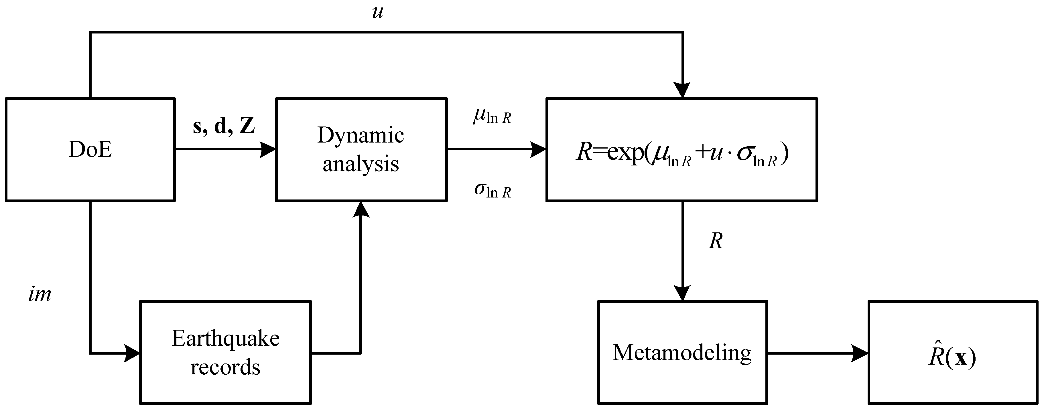
3.1. Metamodel of the EDP

In the proposed method, the uncertainties of ground motions are described by the randomness of IM and record-to-record variation. The IM variable im is treated as a random parameter. An EDP is a quantity to measure the structural response of the dynamic analysis model, such as the maximum inter-storey drift angle and base shear [34]. In seismic reliability assessment, the safety state of a structure is usually judged based on whether EDP R exceeds threshold z, and the failure probability [11] can be expressed as follows:

$$p_f={\displaystyle \int \mathrm{Pr}\{R>z|\mathrm{IM}=im\}{f}_{\mathrm{IM}}(im)}\mathrm{d}(im)$$

(10)

where $f_{\mathrm{IM}}(im)$ represents the probability density function of IM. The conditional probability $\mathrm{Pr}\{R>z|\mathrm{IM}=im\}$ is affected by the record-to-record variation. To tackle this variation, the same seismic demand assumption as in D-RSM-SRA [16] is adopted. In other words, given the IM variable and structural parameters (including d, Z and the structural random parameter s), EDP R is a random variable, for which its statistical properties can be expressed by the mean and variance [11]. Based on this assumption, the record-to-record variation can be implicitly incorporated in a set of ground motion records [18]. In this study, EDP is considered to be lognormally distributed [35]. At each sample in DoE, the mean ${\mu }_{\ln R}$ and standard deviation ${\sigma }_{\ln R}$ of the logarithms of EDP can be obtained by performing NLTHA for all selected records [20].

GPR [36] is a nonparametric statistical method for data fitting with GP. It is suitable for small-sample learning [37]. Common machine learning methods also include linear regression, ridge regression, and logistic regression [38,39]. Compared with other machine learning methods, GPR can analyze the error of the predicted value [40]. Therefore, GPR is employed for metamodeling in the developed method. For a function F(x) to be fitted, the GPR model is built based on a DoE composed of a group of experiments X = [x⁽¹⁾, x⁽²⁾, …, x^(m)] and their outputs y = [y⁽¹⁾, y⁽²⁾, …, y^(m)]^T, where x⁽ⁱ⁾ represents a n-dimensional input vector and y⁽ⁱ⁾ represents its output. At a test point ${\mathbf{x}}_{*}$, the joint prior distribution of y and $F({\mathbf{x}}_{*})$ is as follows:

$$\left[\begin{array}{l}\mathbf{y}\\ F({\mathbf{x}}_{*})\end{array}\right]~\mathrm{N}\left(0,\left[\begin{array}{cc}K(\mathbf{X},\mathbf{X})+{\sigma }_N{}^2{\mathbf{I}}_m& K(\mathbf{X},{\mathbf{x}}_{*})\\ K({\mathbf{x}}_{*},\mathbf{X})& k({\mathbf{x}}_{*},{\mathbf{x}}_{*})\end{array}\right]\right)$$

(11)

where σ_N represents the standard deviation of the normally distributed noise; K(X, X) = [k_ij]_m×m is the covariance matrix and k_ij = k(x⁽ⁱ⁾, x^(j)) is the covariance between x⁽ⁱ⁾ and x^(j); $K(\mathbf{X},{\mathbf{x}}_{*})=K{({\mathbf{x}}_{*},\mathbf{X})}^{\mathrm{T}}$ is the m × 1 covariance matrix between ${\mathbf{x}}_{*}$ and X; and I_m is the m-dimensional identity matrix. The prediction $\widehat{F}({\mathbf{x}}_{*})$ and predicted variance ${\sigma }_{\widehat{F}}^2({\mathbf{x}}_{*})$ of ${\mathbf{x}}_{*}$ are obtained by the following formulas:

$$\widehat{F}({\mathbf{x}}_{*})=K({\mathbf{x}}_{*},\mathbf{X}){[K(\mathbf{X},\mathbf{X})+{\sigma }_N{}^2{\mathbf{I}}_m]}^{-1}\mathbf{y}$$

(12)

and the following.

$${\sigma }_{\widehat{F}}^2({\mathbf{x}}_{*})=k({\mathbf{x}}_{*},{\mathbf{x}}_{*})-K({\mathbf{x}}_{*},\mathbf{X}){[K(\mathbf{X},\mathbf{X})+{\sigma }_N{}^2{\mathbf{I}}_m]}^{-1}K(\mathbf{X},{\mathbf{x}}_{*})$$

(13)

In the GPR model, $F({\mathbf{x}}_{*})$ is considered to follow the normal distribution as follows.

$$F({\mathbf{x}}_{*})~N(\widehat{F}({\mathbf{x}}_{*}),{\sigma }_{\widehat{F}}^2({\mathbf{x}}_{*}))$$

(14)

The square exponential covariance function [41,42] is adopted in this article.

A metamodel for estimating EDP is established in the proposed procedure. To facilitate the prediction of the estimation error, the proposed method does not build the metamodel of the mean ${\mu }_{\ln R}$ and standard deviation ${\sigma }_{\ln R}$ as in the dual RSM framework but employs a GPR model to obtain the structural response. In terms of the assumption of lognormally distributed seismic demand, when d, Z, s, and im are fixed, the value of the EDP is expressed as follows.

$$R=\exp [{\mu }_{\ln R}+\mathrm{N}(0,{\sigma }_{\ln R}{}^2\left)\right]$$

(15)

The normally distributed variable $\mathrm{N}(0,{\sigma }_{\ln R}{}^2)$ can be converted to $u\cdot {\sigma }_{\ln R}$, where u follows the standard normal distribution. Then, Formula (15) is transformed into the following.

$$R=\exp ({\mu }_{\ln R}+u\cdot {\sigma }_{\ln R})$$

(16)

The input variable x of the EDP’s metamodel consists of d, Z and P, i.e., x = [d, Z, P]. Variable u related to the randomness of seismic demand is regarded as a random parameter, and structural random parameter s is also included in P. By choosing samples in x space and calculating their corresponding R values according to Formula (16), DoE can be generated. Based on the DoE, the GPR model of EDP is constructed, which can provide the prediction $\widehat{R}(\mathbf{x})$ and prediction error ${\sigma }_{\widehat{R}}(\mathbf{x})$ of the response. The schematic of modeling for the EDP is shown in Figure 1.

For a given design variable D = [d,μ_Z], by combining d with N points randomly generated according to the distribution parameters of Z and P, MCS samples X^MC = [${\mathbf{x}}_1^{\mathrm{MC}}$, ${\mathbf{x}}_2^{\mathrm{MC}}$, …, ${\mathbf{x}}_N^{\mathrm{MC}}$] are obtained. Then, the failure probability that the response exceeds the threshold z can be estimated by the following:

$${\widehat{p}}_f(\mathbf{D})=\frac{{\displaystyle \sum _{j=1}^{N}I[z-\widehat{R}({\mathbf{x}}_j^{\mathrm{MC}})]}}{N}$$

(17)

where $I(\cdot )$ is an indicator function for counting the number of negative values. When the value in the brackets is negative, the value of $I(\cdot )$ is 1; otherwise, it is 0.

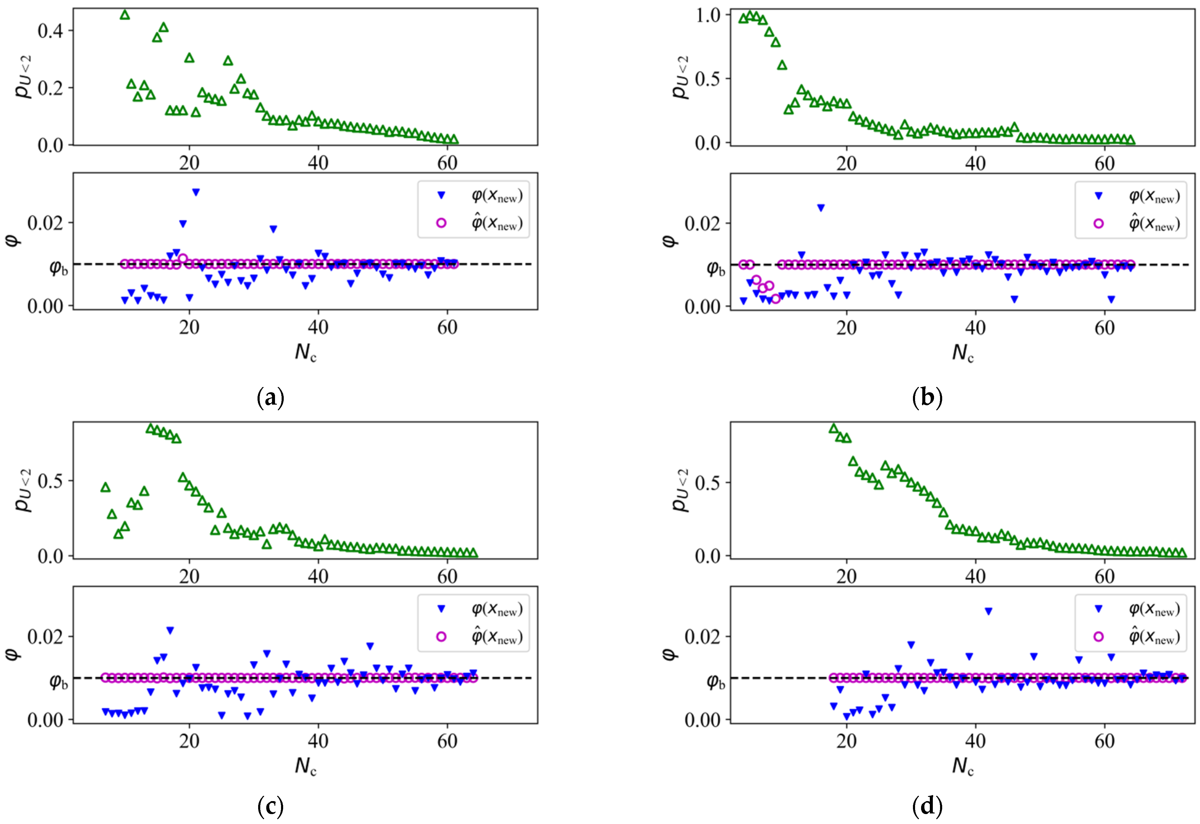
3.2. Refinement of the Metamodel

Based on the metamodel of EDP, RBDO methods such as EGO-EGRA can be used to obtain the optimal solution of the problem. However, EGO-EGRA does not consider the influence of probability density in updating DoE, which may result in unnecessary calculation cost. In order to further reduce computational burden, this study presents an AL strategy to improve the EGO-EGRA method. AL has been widely used in reliability analysis [43,44]. Such strategies update DoE by selecting new samples based on the learning function value of each point in the candidate set.

Since Latin hypercube sampling (LHS) [45] has the advantage of avoiding excessive aggregation of samples, initial experiments are uniformly sampled in the upper and lower bounds of each variable by LHS. In order to accurately predict the safety states of most MCS points, the sampling range of DoE should be a region where the points with large joint probability density can fall. The bounds of the i-th random parameter P_i in P can be taken as $F_i^{-1}[\Phi (\pm 4)]$, where $F_i^{-1}(\cdot )$ is the inverse function of the probability distribution function of P_i. The sampling ranges of d and Z can be the bounds in the optimization problem. The size of the initial DoE can be close to the number of input variables of the metamodel.

After the initial metamodel is established, AL is used in the proposed method to select new sample points to update DoE. A candidate point set X^c = [${\mathbf{x}}_1^{\mathrm{c}}$, ${\mathbf{x}}_2^{\mathrm{c}}$, …, ${\mathbf{x}}_r^{\mathrm{c}}$] for refining the metamodel needs to be first generated without calculating the corresponding responses. The accuracy of the model at the location where MCS random points are very sparse has little influence on the reliability results; thus, there is no need to sample many candidate points with a small joint probability density. The candidate set is chosen by LHS according to the statistical characteristics of the variables, which is obtained as follows: a set of points Q = [q_i]_r =[q_ij]_r×n is uniformly generated in the space of (0, 1)ⁿ using LHS, and candidate set X^c is obtained by transforming [9] Q as follows.

$${\mathbf{X}}^c={[{\mathbf{x}}_i^{\mathrm{c}}]}_r={[F_i^{-1}(q_{ij})]}_{r\times n}$$

(18)

In this transformation, Z and P can be treated as uniformly distributed variables.

By selecting the candidate point that is most favorable for refining the metamodel as the new sample ${\mathbf{x}}_{new}$, DoE is updated once. The model can be gradually refined by sampling new experiment from the candidate set sequentially. The new sample ${\mathbf{x}}_{new}$ is picked in terms of the learning function values of the candidate points. It can be observed from Formula (17) that the accuracy of the metamodel near the limit state surface R = z has a great influence on the judgment of the sign of $z-\widehat{R}$. Therefore, more attention should be paid to accuracy in this area. Due to the characteristics of the GPR model, if the prediction error at a certain point is large and the point may be in the vicinity of the limit state, adding this point to DoE can improve the accuracy of $\widehat{R}(\mathbf{x})$ in the neighborhood of z. The learning function should be able to identify such points. The U function is a commonly used learning function [44]. For the metamodel of the seismic demand, the U function can be expressed as follows

$$U(\mathbf{x})=\left|\frac{z-\widehat{R}(\mathbf{x})}{{\sigma }_{\widehat{R}}(\mathbf{x})}\right|$$

(19)

It can be observed from Formula (19) that the closer the approximate response of a point is to z and the greater the predicted error is, and the smaller the U function value is. Therefore, the point with the minimum value of U function in the candidate set is chosen as the new sample ${\mathbf{x}}_{new}$. It can be described as follows.

$${\mathbf{x}}_{new}=\underset{\mathbf{x}\in {\mathbf{X}}^{\mathrm{c}}}{\arg \min }(U(\mathbf{x}))$$

(20)

According to Ref. [43], the error rate of safety state judgment of a point with the metamodel is less than 2.3% if the U function value of this point is greater than 2, and sampling can be stopped when the U function values of all candidate points are greater than 2. This stop condition is too strict for the engineering issues concerned in this study; thus, a more relaxed condition is adopted. In the developed method, whether to stop sampling is determined according to the proportion $p_{U<2}$ of candidate points with U function value less than 2. Here, $p_{U<2}$ is described as follows:

$$p_{U<2}=\frac{N_{U<2}}{r}=\frac{{\displaystyle \sum _{k=1}^{r}I[U({\mathbf{x}}_k^{\mathrm{c}})-2]}}{r}$$

(21)

where $N_{U<2}$ represents the number of points for which its U function is less than 2 in the candidate set. When $p_{U<2}$ is less than a certain tolerance ζ, the metamodel is considered to be sufficiently accurate. ζ is taken as 0.02 in this paper.

After the metamodel of EDP is refined, RBDO problems (1) or (2) can be transformed into the form in Formulas (8) or (9) by Formula (17), and the optimal solution can be obtained by using EGO. It can be observed from the steps of the proposed method that the number of calls to FEA in optimization depends on the number of experiments for establishing the metamodel of EDP.

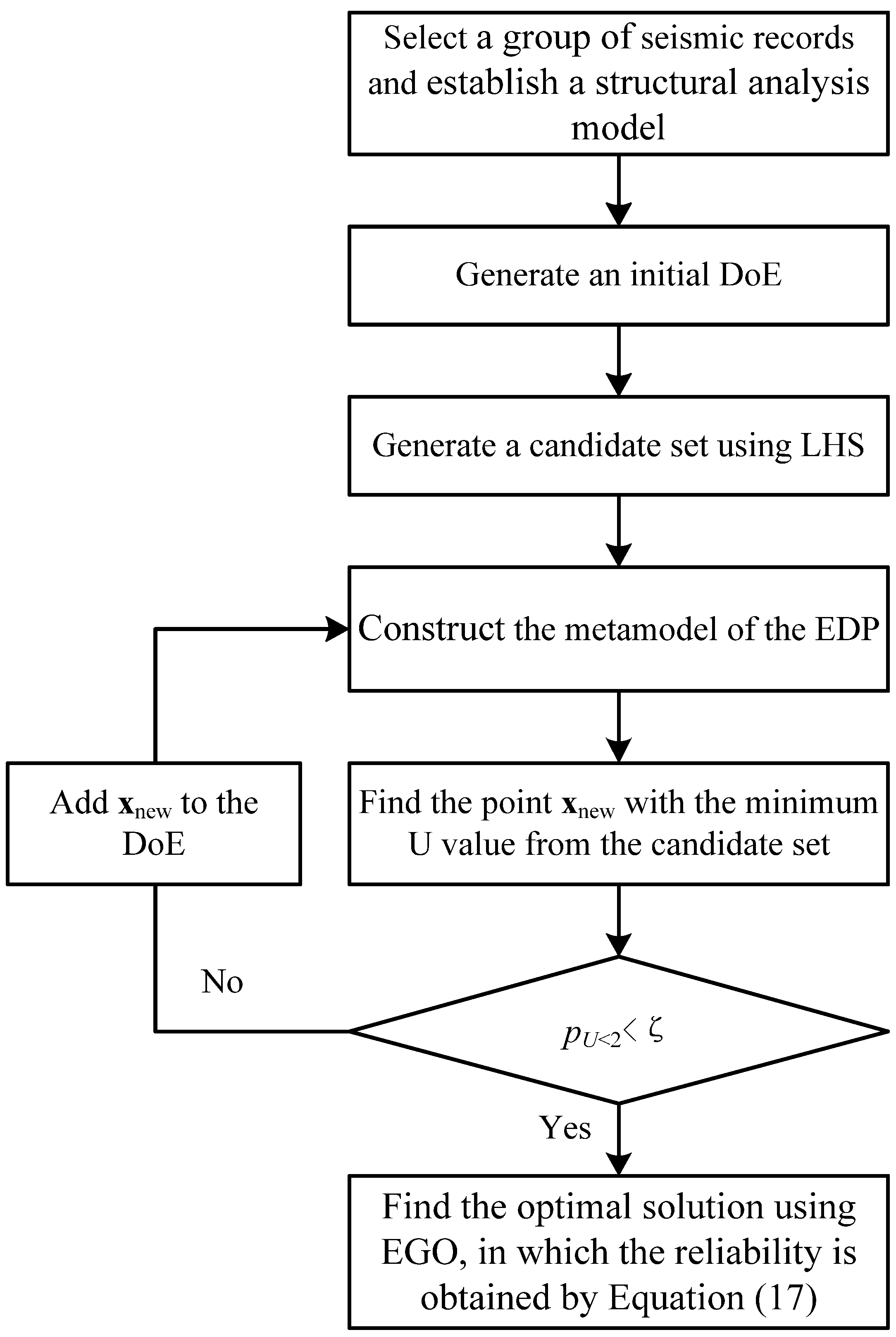
3.3. Computational Procedure of RBDO

The proposed RBDO framework of structures subjected to earthquake load involves the following basic steps, and its flowchart is shown in Figure 2:

(1)

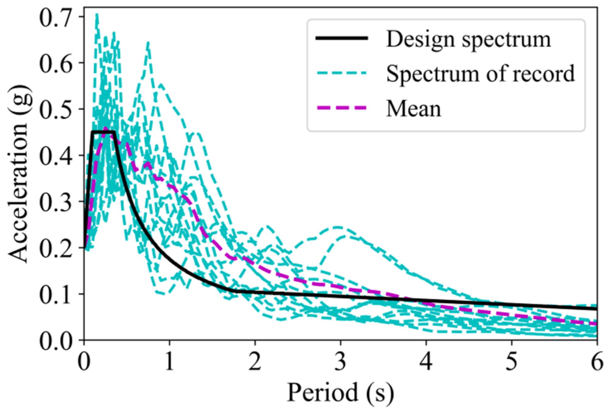
Select a group of seismic records and establish a structural analysis model.

(2)

Generate an initial DoE: sample n_s (e.g., the number of the input variables) initial experiments in the space of x = [d, Z, P] by LHS, perform NLTHA for all selected records at each sample, and calculate the seismic demand according to Formula (16).

(3)

In terms of Formula (18), use LHS to choose a candidate set containing r points (r = 10,000 in this research).

(4)

Construct the GPR model of EDP with DoE.

(5)

Pick the point ${\mathbf{x}}_{new}$ with the minimum value of U function from the candidate set according to Formula (20). If $p_{U<2}$ < ζ (ζ is taken as 0.02), proceed to step (6); otherwise, add the new sample ${\mathbf{x}}_{new}$ with its seismic demand to the DoE, and return to step (4).

(6)

By Formula (17), transform RBDO problems (1) or (2) into the form in Formulas (8) or (9) and search for the optimal solution using the EGO algorithm.

4. Numerical Studies

To validate the effectiveness and efficiency of the proposed method, it is applied to two illustrative examples: one is to reduce the costs of a steel frame under the probability constraint, and the other is to improve the reliability of a reinforced concrete frame under the cost constraint. The results were compared with MCS and EGO-EGRA. MCS is usually considered to be a highly accurate reliability calculation method; thus, it is used here to test the accuracy of other methods. Since calculation time is mainly spent on the NLTHA, computational efficiency is measured by the number N_c of calls to FEA. N_c is equal to the number of samples for constructing the metamodel of the EDP. In an FEA, the NLTHA is carried out for all selected earthquake records.

In the examples, the assumptions of distribution types commonly used in existing studies are adopted for IM and structural parameters. For practical engineering problems, whether a random variable follows the assumed distribution type can be evaluated by goodness-of-fit tests, such as Anderson–Darling statistic [46]. In the problems in this section, peak ground acceleration (PGA) a is selected as the IM. The ground motion parameters are considered to be Type I or Type II extreme value distributed in Cornell’s research [47]. In this study, the PGA in a future period of time t is assumed to follow the Type II extreme value distribution, and its probability distribution function [48] is as follows:

$$F_a(a)=\exp \left[-\frac{t}{T}{\left(\frac{a}{a_{\mathrm{g}}}\right)}^{-K}\right]$$

(22)

where T represents the design reference period, $a_{\mathrm{g}}$ denotes the mode value of acceleration, and K represents the shape parameter. t/T is taken as 1 here, and then the mean ${\mu }_a$, standard deviation ${\sigma }_a$ and coefficient of variation $C_a$ of PGA are as follows.

$${\mu }_a=a_{\mathrm{g}}\Gamma (1-\frac{1}{K})$$

(23)

$${\sigma }_a=a_{\mathrm{g}}{\left[\Gamma (1-\frac{2}{K})-{\Gamma }^2(1-\frac{1}{K})\right]}^{\frac{1}{2}}$$

(24)

$$C_a={\left[\Gamma (1-\frac{2}{K})/{\Gamma }^2(1-\frac{1}{K})-1\right]}^{\frac{1}{2}}$$

(25)

Gao et al. carried out statistics on the seismic hazard of 45 cities, and the data show the following: ${\mu }_a=0.597a_{\mathrm{k}}$, $C_a=1.176$; here, $a_{\mathrm{k}}$ represents the basic design acceleration, which is the acceleration value with an exceedance probability of 10% within the design reference period of 50 years [49]. Accordingly, K = 2.40 and $a_{\mathrm{g}}=0.391a_{\mathrm{k}}$ [50]. It is assumed that the seismic fortification intensity is 8 and the site classification is II. The damping ratio of the structures is 0.05. With reference to the current Chinese code for seismic design of buildings (GB50011-2010) [51], $a_{\mathrm{k}}$ is taken as 0.2 g. Then, the mean of a is 1.17 m/s².

About 10~20 earthquake records are required for dynamic analysis to evaluate the seismic performance of structures [52]. Therefore, 20 seismic records for NLTHA were chosen from the ground motion database of PEER Center, taking the design spectrum in GB50011-2010 as the target spectrum. The information of these ground motions is listed in

Table 1. Earthquake records.

No.	Earthquake Name	Year	Station Name	Arias Intensity (m/s)	Magnitude
1	Cape Mendocino	1992	Eureka—Myrtle and West	0.3	7.01
2	Cape Mendocino	1992	Fortuna—Fortuna Blvd	0.3	7.01
3	Landers	1992	Yermo Fire Station	0.9	7.28
4	Northridge-01	1994	Downey—Co Maint Bldg	0.6	6.69
5	Northridge-01	1994	Hollywood—Willoughby Ave	0.9	6.69
6	Northridge-01	1994	LA—Baldwin Hills	0.7	6.69
7	Northridge-01	1994	Moorpark—Fire Sta	0.9	6.69
8	Kocaeli_ Turkey	1999	Iznik	0.4	7.51
9	Cape Mendocino	1992	College of the Redwoods	0.6	7.01
10	Chuetsu-oki_ Japan	2007	Joetsu Ogataku	0.7	6.8
11	Chuetsu-oki_ Japan	2007	Sanjo Shinbori	2	6.8
12	Chuetsu-oki_ Japan	2007	Nakanoshima Nagaoka	2.1	6.8
13	Chuetsu-oki_ Japan	2007	Yan Sakuramachi City watershed	0.7	6.8
14	Iwate_ Japan	2008	Kami_ Miyagi Miyazaki City	0.4	6.9
15	Iwate_ Japan	2008	Matsuyama City	1.2	6.9
16	Iwate_ Japan	2008	Iwadeyama	1.8	6.9
17	Iwate_ Japan	2008	Misato_ Miyagi Kitaura—B	0.7	6.9
18	Iwate_ Japan	2008	Minamikatamachi Tore City	1.4	6.9
19	Iwate_ Japan	2008	Yokote Masuda Tamati Masu	0.3	6.9
20	Iwate_ Japan	2008	Yokote Ju Monjimachi	0.4	6.9

, and the design spectrum and mean spectrum of the selected records are plotted in Figure 3. NLTHA was carried out in OpenSeespy (the version of OpenSees for Python).

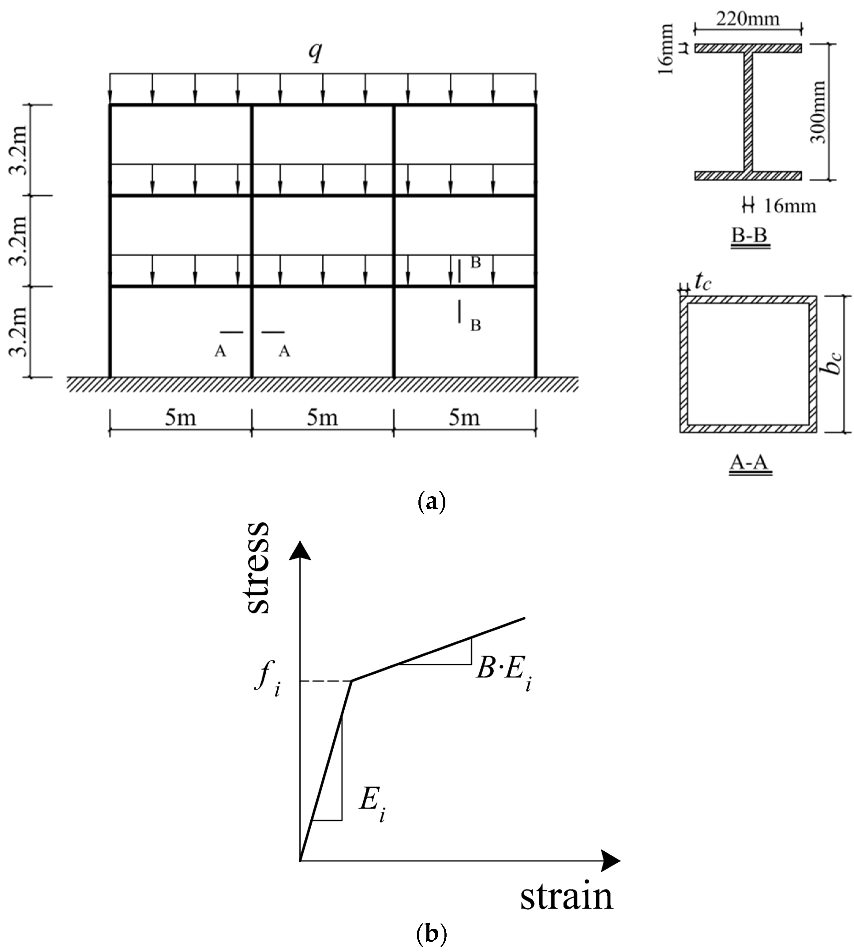
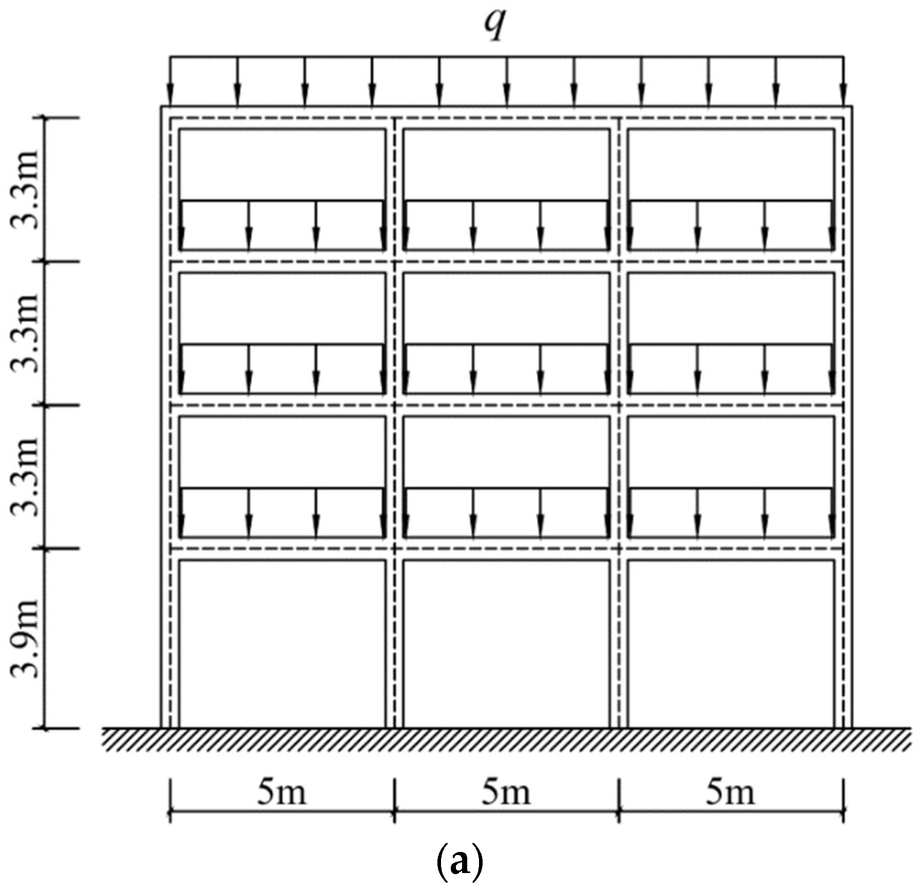
4.1. Example 1: A Steel Frame

Figure 4a shows a three-storey steel frame for which its storey height is 3.2 m and bay width is 5 m. The density of steel is 7850 kg/m³. The uniformly distributed load q on beams is 30.0 kN/m. A wide flange cross-section is adopted for the beam. The section depth is 0.3 m, the web thickness is 0.016 m, and the flange width and thickness are 0.22 m and 0.016 m, respectively. A square tube section with a width of b_c and wall thickness of t_c is adopted for the column. The beam and column members are modeled using displacement-based beam–column elements. The bilinear model is employed to simulate the nonlinear properties of steel [53], as shown in Figure 4b. The ratio of post-yield to initial stiffness B is 0.02. The initial elastic modulus and yield strength of the column steel are E₁ and f₁, respectively. The initial elastic modulus and yield strength of the beam steel are E₂ and f₂, respectively.

As inter-storey drift is often used to evaluate the seismic performance of structures [54], it is selected as the failure criterion in this study where the maximum inter-storey drift angle φ of the structure under earthquake load exceeds the deformation limit φ_b. With reference to the evaluation standard for moderate damage of steel frames in GB50011-2010, deformation limit φ_b is taken as 1/100 in this example.

In addition to the uncertainty of earthquakes, the randomness of E₁, E₂, f₁, f₂, and t_c is also considered in this optimization problem. E₁, E₂, f₁, and f₂ are random parameters; t_c is a random design variable with a mean of ${\mu }_{t_{\mathrm{c}}}$. Their distribution information is shown in

Table 2. Random design variables and parameters in Example 1.

Variable	Distribution Type	Mean	Standard Deviation
f1 (Pa)	Lognormal	3 × 108	3 × 107
f2 (Pa)	Lognormal	3 × 108	3 × 107
E1 (Pa)	Lognormal	2 × 1011	2 × 1010
E2 (Pa)	Lognormal	2 × 1011	2 × 1010
u	Normal	0	1
a (m/s2)	Type II extreme value	1.17	1.376
tc (m)	Lognormal	${\mu }_{t_{\mathrm{c}}}$	0.05·${\mu }_{t_{\mathrm{c}}}$

. Since the column parameters have a great impact on seismic resistance, the width b_c and the thickness mean value ${\mu }_{t_{\mathrm{c}}}$ are taken as design variables. The bounds of b_c and ${\mu }_{t_{\mathrm{c}}}$ are [0.22, 0.5] m and [0.01, 0.02] m, respectively. Generally, the failure probability of a structural component is required to be less than 0.05 in civil engineering [7]. In this optimization problem, the failure probability of the structure is limited to less than 0.05, and the column section area S_c is selected as the optimization objective to minimize the costs. The RBDO problem can be described as follows.

$$\begin{array}{l}\mathrm{Find}: \mathbf{D}=[b_{\mathrm{c}},{\mu }_{t_{\mathrm{c}}}{]}^{\mathrm{T}}\\ \mathrm{Minimize}: S_{\mathrm{c}}(b_{\mathrm{c}},{\mu }_{t_{\mathrm{c}}})=b_{\mathrm{c}}{}^2-{(b_{\mathrm{c}}-2{\mu }_{t_{\mathrm{c}}})}^2\\ \mathrm{Subject} \mathrm{to}: \mathrm{Pr}\{\phi (f_1,f_2,E_1,E_2,u,a,b_{\mathrm{c}},t_{\mathrm{c}})\ge 1/100\}\le 0.05\end{array}$$

(26)

The values of b_c and ${\mu }_{t_{\mathrm{c}}}$ in the initial scenario are 0.25 m and 0.016 m, respectively.

The proposed method was used to solve this optimization problem. Nine initial experiments for establishing the metamodel of the EDP were chosen, which are listed in

Table 3. Initial DoE of the EDP in Example 1.

No.	Input Variable Vector x								φ
	f1 (108 Pa)	f2 (108 Pa)	E1 (1011 Pa)	E2 (1011 Pa)	u	a (m/s2)	bc (m)	tc (m)
1	2.614	4.143	2.339	1.636	1	2.59	0.395	0.01875	0.00785
2	4.143	3.837	1.837	1.837	−2	4.86	0.5	0.01125	0.00697
3	3.837	2.309	2.439	2.138	3	9.39	0.465	0.015	0.03796
4	2.003	3.532	1.636	2.038	4	13.92	0.36	0.01625	0.28035
5	4.449	2.92	2.138	1.937	0	18.45	0.29	0.02	0.06172
6	3.532	4.449	2.038	2.339	2	7.12	0.22	0.01375	0.12321
7	2.92	2.003	1.937	1.736	−1	11.65	0.255	0.01	0.03365
8	2.309	3.226	2.239	2.439	−3	16.18	0.43	0.0125	0.01047
9	3.226	2.614	1.736	2.239	−4	0.33	0.325	0.0175	0.00025

. A candidate set containing 10,000 points was generated, and their distribution in f₁-f₂-E₁ space is shown in Figure 5. A total of 52 samples were added during AL sampling, and the iteration history of sampling is shown in Figure 6a. It can be observed that the response predictions of the new samples were mostly located in the vicinity of the threshold φ_b. With the expansion of the size of DoE, the difference between $\phi (x_{new})$ and $\widehat{\phi }(x_{new})$ gradually decreased, and the value of $p_{U<2}$ decreased with fluctuations. After establishing the metamodel, the failure probability corresponding to design variable D could be obtained. The failure probability values obtained by the proposed method were compared with those by MCS and EGO-EGRA. The simulation samples of MCS were selected by LHS. According to Ref. [10], 200 samples generated using LHS are sufficient to ensure the accuracy of the MCS results for seismic reliability calculation; thus, 1000 simulation points were selected in this work. The reliability values of 25 groups of design variables were calculated, and the number of calls to FEA in MCS is 25,000 and that number in EGO-EGRA is 120. The reliability results obtained by different methods are plotted in Figure 7. The three surfaces are very close to each other, which verifies the accuracy of the reliability information provided by the proposed method.

Based on the metamodel of the EDP, the original RBDO problem could be transformed into the form of Formula (8), and the optimal solution was obtained using EGO. The optimization results of the proposed method and EGO-EGRA are listed in

Table 4. Optimization results of Example 1.

Method	Nc	Design Variable Vector D		Sc (m2)	${\hat{\mathit{p}}}_{\mathit{f}}$
		bc (m)	${\mathit{\mu }}_{{\mathit{t}}_{\mathbf{c}}} \left(\mathbf{m}\right)$
EGO-EGRA	120	0.3322	0.01	0.01289	0.0481
Proposed method	9 + 52	0.3300	0.01	0.01280	0.0497
	3 + 61	0.3302	0.01	0.01281	0.0496
	6 + 58	0.3304	0.01	0.01282	0.0496
	17 + 55	0.3321	0.01	0.01288	0.0483
Initial scenario	-	0.25	0.016	0.01498	0.0914

. After optimization, the cross-section area of column was reduced from 0.015 m² to 0.0128 m², and the failure probability was less than 5%. The result of the proposed method is close to that of EGO-EGRA, but the calculation cost is less, which validates the efficiency and accuracy of this method.

In addition, the optimization problem was solved using the proposed method in another three different cases, where the numbers of initial experiments, N_I, were 3, 6, and 17, respectively. The changes in $\phi ({\mathbf{x}}_{new})$, $\widehat{\phi }({\mathbf{x}}_{new})$, and $p_{U<2}$ in the sampling processes are shown in Figure 6b–d. The difference between the four solutions of the proposed method is small, which indicates that this method is insensitive to the number of initial samples and can obtain optimization results stably.

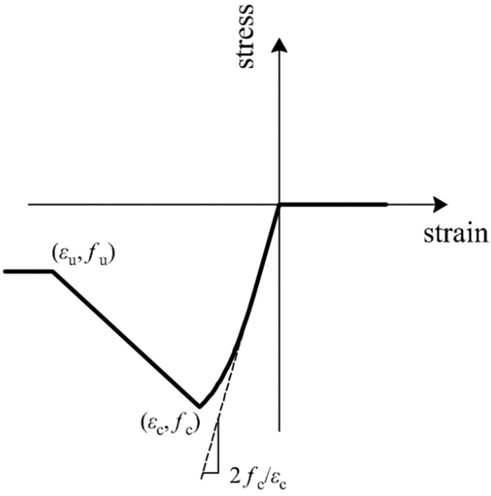
4.2. Example 2: A Reinforced Concrete Frame

This example is a four-storey reinforced concrete frame, as shown in Figure 8. The height of the first floor is 3.9 m, and the height of other floors is 3.3 m. The width of the bay is 5 m. The density of concrete is 2550 kg/m³. The uniformly distributed load q on the structure is 35 kN/m. The cross-section of the member is composed of steel reinforcement, cover concrete, and core concrete. The diameter of rebar is 28 mm. The thickness of the cover concrete is 0.03 m. The cross-section of beam is a rectangle with a size of 0.4 m × 0.6 m. A square cross-section is adopted for the column. The width of the column section of the first floor is b₁; the column cross-sections of the second, third, and fourth floor are the same, the width of which is b₂. The material properties of the steel bar are simulated using a bilinear model. The initial elastic modulus and yield strength of the steel are E_s and f_s, respectively, and the ratio of the post-yield to the initial stiffness is 0.05. The Kent–Scott–Park model is employed to simulate the nonlinear characteristics of concrete [53], as shown in Figure 9. The compressive strength of the cover concrete, f_c,cover, is 2.758 × 10⁷ Pa, and the strain at maximum strength ε_c,cover is 0.002; the crushing strength f_u,cover is 0, and the strain at crushing strength ε_u,cover is 0.06. The crushing strength of the core concrete, f_u,core, is 2.413 × 10⁷ Pa [2], and the strain at maximum strength ε_u,core is 0.02; the compressive strength and strain at maximum strength are f_c,core and ε_c,core.

According to the evaluation standard for the moderate damage of reinforced concrete frames in GB50011-2010, deformation limit φ_b is taken as 1/120. In this RBDO problem, b₁ and b₂ are regarded as deterministic random variables, and the bounds are $b_1,b_2\in \left[0.3,0.5\right] \mathrm{m}$. The randomness of material property parameters f_s, E_s, f_c, and ε_u,core are considered, and the distribution information of the random parameters is shown in

Table 5. Random parameters in Example 2.

Variable	Distribution Type	Mean	Standard Deviation
fs (Pa)	Lognormal	3.07 × 108	3.07 × 107
fc (Pa)	Lognormal	3.447 × 107	3.447 × 106
Es (Pa)	Lognormal	2.01 × 1011	2.01 × 1010
εu,core	Lognormal	5 × 10−3	5 × 10−4
u	Normal	0	1
a (m/s2)	Type II extreme value	1.17	1.376

. In the initial scenario, b₁ and b₂ are 0.33 m and 0.43 m, respectively. The optimization objective is to maximize the reliability of the structure, and the total volume V_c of columns is required not to exceed the column volume V_c0 of the initial scenario. The RBDO problem can be described as follows.

$$\begin{array}{l}\mathrm{Find}: \mathbf{D}=[b_1,b_2{]}^{\mathrm{T}}\\ \mathrm{Minimize}: \mathrm{Pr}\{\phi (f_s,f_c,E_s,{\epsilon }_{\mathrm{u},\mathrm{core}},u,a,b_1,b_2)\ge 1/120\}\\ \mathrm{Subject} \mathrm{to}: V_{\mathrm{c}}\le V_{\mathrm{c}0}\end{array}$$

(27)

The proposed method was used to find the optimal solution of the problem. The initial DoE contained nine sample points, as listed in

Table 6. Initial DoE of the EDP in Example 2.

No.	Input Variable Vector x								φ(x)
	fs (108 Pa)	fc (107 Pa)	Es (1011 Pa)	εu,core (10−3)	u	a (m/s2)	b1 (m)	b2 (m)
1	2.363	4.76	1.342	5.377	3	6.18	0.35	0.375	0.1648
2	4.24	4.409	2.571	7.415	1	4.23	0.425	0.3	0.02113
3	2.988	5.112	2.981	4.867	−3	10.08	0.45	0.425	0.00566
4	3.614	3.707	1.957	3.338	−4	2.28	0.3	0.4	0.00139
5	3.927	2.301	2.776	4.357	4	8.13	0.375	0.475	0.28316
6	4.553	4.058	1.547	6.396	−2	12.03	0.4	0.5	0.01429
7	3.301	3.355	1.752	3.848	2	13.98	0.5	0.325	0.22224
8	2.675	2.653	2.366	6.905	−1	15.93	0.325	0.35	0.04925
9	2.05	3.004	2.161	5.886	0	0.34	0.475	0.45	0.00066

. According to Formula (18), 1000 candidate points were generated. A total of 101 samples were added in the iterative process of AL sampling, as shown in Figure 10. The failure probabilities corresponding to the design variables obtained by MCS, EGO-EGRA, and the proposed method are plotted in Figure 11. The number of calls to FEA in MCS is 25,000 and that in EGO-EGRA is 196. It can be observed that the reliability information given by the proposed method is close to that of MCS, but the computational burden is far less than that of the latter.

Once the metamodel was built, the optimization problem could be transformed into the form of Formula (9), and the EGO algorithm was used to obtain the optimal solution, which is listed in

Table 7. Optimization results of Example 2.

Method	Nc	Design Variable Vector D		Vc (m3)	${\hat{\mathit{p}}}_{\mathit{f}}$
		b1 (m)	b2 (m)
EGO-EGRA	196	0.448	0.386	9.02	0.0424
Proposed method	9 + 101	0.442	0.388	9.02	0.0423
Initial scenario	-	0.33	0.43	9.02	0.096

. The result of EGO-EGRA is also given in this table, which shows that the solution obtained by this method is close to that by EGO-EGRA. After optimization, the failure probability of the structure decreased from 9.6% to 4.2%, and the materials used in the structure did not increase. The example indicates that the proposed method is also applicable to the problem of taking seismic reliability as the optimization objective.

5. Conclusions

In order to effectively consider the uncertainties of ground motions and structural parameters with appropriate computation cost in optimization problems, an efficient RBDO method for structures under earthquake load based on adaptive metamodeling is proposed. In this method, the uncertainties of ground motions are expressed by the record-to-record variation and the randomness of IM. GPR is used to estimate the seismic demand of the structure, and MCS is employed to calculate the failure probability of the design variables. An AL sampling strategy is presented to refine the metamodel of the EDP. Based on approximate reliability, the optimal solution of the RBDO problem can be obtained by the EGO algorithm.

The developed method was applied to a steel frame and a reinforced concrete frame, respectively, in which the randomness of material properties was considered, and the analysis results are compared with those of the MCS and EGO-EGRA methods. The results show that this method can adaptively improve DoE according to the complexity of the problem. It can tackle the problems of minimizing costs under the reliability constraint and problems of improving the seismic reliability under limited costs. The reliability information obtained by this method is very close to that of MCS, but the number of calls to FEA is much less than that of MCS. The difference between the optimization result obtained by the proposed method and that by EGO-EGRA is small, but this method shows higher efficiency. In addition, the number of initial samples has little impact on the results of the proposed procedure, and the optimal solution can be obtained stably.

The proposed method provides a foundation for future research on optimization problems considering the robustness of seismic performance of complex structures.

References

1. FEMA-356; Prestandard and Commentary for the Seismic Rehabilitation of Buildings. Federal Emergency Management Agency: Washington, DC, USA, 2000.
2. Ni, P.; Li, J.; Hao, H.; Yan, W.; Du, X.; Zhou, H. Reliability analysis and design optimization of nonlinear structures. Reliab. Eng. Syst. Saf. 2020, 198, 106860. [Google Scholar] [CrossRef]
3. Yazdani, H.; Khatibinia, M.; Gharehbaghi, S.; Hatami, K. Probabilistic performance-based optimum seismic design of RC structures considering soil–structure interaction effects. ASCE-ASME J. Risk Uncertain. Eng. Syst. Part A Civ. Eng. 2017, 3, G4016004. [Google Scholar] [CrossRef]
4. Zou, X.; Wang, Q.; Wu, J. Reliability-based performance design optimization for seismic retrofit of reinforced concrete buildings with fiber-reinforced polymer composites. Adv. Struct. Eng. 2018, 21, 838–851. [Google Scholar] [CrossRef]
5. Mishra, S.K.; Roy, B.K.; Chakraborty, S. Reliability-based-design-optimization of base isolated buildings considering stochastic system parameters subjected to random earthquakes. Int. J. Mech. Sci. 2013, 75, 123–133. [Google Scholar] [CrossRef]
6. Hadidi, A.; Azar, B.F.; Rafiee, A. Reliability-based design of semi-rigidly connected base-isolated buildings subjected to stochastic near-fault excitations. Earthq. Struct. 2016, 11, 701–721. [Google Scholar] [CrossRef]
7. Peng, Y.; Ma, Y.; Huang, T.; De Domenico, D. Reliability-based design optimization of adaptive sliding base isolation system for improving seismic performance of structures. Reliab. Eng. Syst. Saf. 2021, 205, 107167. [Google Scholar] [CrossRef]
8. FEMA P695; Quantification of Building Seismic Performance Factors. Federal Emergency Management Agency: Washington, DC, USA, 2009.
9. Su, L.; Li, X.L.; Jiang, Y.P. Comparison of methodologies for seismic fragility analysis of unreinforced masonry buildings considering epistemic uncertainty. Eng. Struct. 2020, 205, 110059. [Google Scholar] [CrossRef]
10. Dolsek, M. Incremental dynamic analysis with consideration of modeling uncertainties. Earthq. Eng. Struct. Dyn. 2009, 38, 805–825. [Google Scholar] [CrossRef]
11. Perotti, F.; Domaneschi, M.; De Grandis, S. The numerical computation of seismic fragility of base-isolated nuclear power plants buildings. Nucl. Eng. Des. 2013, 262, 189–200. [Google Scholar] [CrossRef]
12. Lagaros, N.D.; Fragiadakis, M. Fragility assessment of steel frames using neural networks. Earthq. Spectra 2007, 23, 735–752. [Google Scholar] [CrossRef]
13. Khatibinia, M.; Salajegheh, E.; Salajegheh, J.; Fadaee, M.J. Reliability-based design optimization of reinforced concrete structures including soil–structure interaction using a discrete gravitational search algorithm and a proposed metamodel. Eng. Optim. 2013, 45, 1147–1165. [Google Scholar] [CrossRef]
14. Pang, Y.; Dang, X.; Yuan, W. An artificial neural network based method for seismic fragility analysis of highway bridges. Adv. Struct. Eng. 2014, 17, 413–428. [Google Scholar] [CrossRef]
15. Towashiraporn, P. Building Seismic Fragilities Using Response Surface Metamodels. Ph.D. Thesis, Georgia Institute of Technology, Atlanta, CA, USA, 2004. [Google Scholar]
16. Park, J.; Towashiraporn, P. Rapid seismic damage assessment of railway bridges using the response-surface statistical model. Struct. Saf. 2014, 47, 1–12. [Google Scholar] [CrossRef]
17. Saha, S.K.; Matsagar, V.; Chakraborty, S. Uncertainty quantification and seismic fragility of base-isolated liquid storage tanks using response surface models. Probabilistic Eng. Mech. 2016, 43, 20–35. [Google Scholar] [CrossRef]
18. Ghosh, S.; Ghosh, S.; Chakraborty, S. Seismic reliability analysis of reinforced concrete bridge pier using efficient response surface method–based simulation. Adv. Struct. Eng. 2018, 21, 2326–2339. [Google Scholar] [CrossRef]
19. Zhang, Y.; Wu, G. Seismic vulnerability analysis of RC bridges based on Kriging model. J. Earthq. Eng. 2019, 23, 242–260. [Google Scholar] [CrossRef]
20. Xiao, Y.; Ye, K.; He, W. An improved response surface method for fragility analysis of base-isolated structures considering the correlation of seismic demands on structural components. Bull. Earthq. Eng. 2020, 18, 4039–4059. [Google Scholar] [CrossRef]
21. Datta, G.; Bhattacharjya, S.; Chakraborty, S. Efficient reliability-based robust design optimization of structures under extreme wind in dual response surface framework. Struct. Multidiscip. Optim. 2020, 62, 2711–2730. [Google Scholar] [CrossRef]
22. Liu, H.; Ong, Y.S.; Cai, J. A survey of adaptive sampling for global metamodeling in support of simulation-based complex engineering design. Struct. Multidiscip. Optim. 2018, 57, 393–416. [Google Scholar] [CrossRef]
23. Zhuang, X.; Pan, R. A sequential sampling strategy to improve reliability-based design optimization with implicit constraint functions. J. Mech. Des. 2012, 134, 021002. [Google Scholar] [CrossRef]
24. Bichon, B.J.; Eldred, M.S.; Mahadevan, S.; McFarland, J.M. Efficient global surrogate modeling for reliability-based design optimization. J. Mech. Des. 2013, 135, 011009. [Google Scholar] [CrossRef]
25. Chen, Z.; Qiu, H.; Gao, L.; Li, X.; Li, P. A local adaptive sampling method for reliability-based design optimization using Kriging model. Struct. Multidiscip. Optim. 2014, 49, 401–416. [Google Scholar] [CrossRef]
26. Meng, Z.; Zhang, Z.; Zhang, D.; Yang, D. An active learning method combining Kriging and accelerated chaotic single loop approach (AK-ACSLA) for reliability-based design optimization. Comput. Methods Appl. Mech. Eng. 2019, 357, 112570. [Google Scholar] [CrossRef]
27. Li, G.; Yang, H.; Zhao, G. A new efficient decoupled reliability-based design optimization method with quantiles. Struct. Multidiscip. Optim. 2020, 61, 635–647. [Google Scholar] [CrossRef]
28. Wang, C.; Qiu, Z. Improved numerical prediction and reliability-based optimization of transient heat conduction problem with interval parameters. Struct. Multidiscip. Optim. 2015, 51, 113–123. [Google Scholar] [CrossRef]
29. Wang, C.; Qiu, Z.; Xu, M.; Li, Y. Novel numerical methods for reliability analysis and optimization in engineering fuzzy heat conduction problem. Struct. Multidiscip. Optim. 2017, 56, 1247–1257. [Google Scholar] [CrossRef]
30. Chen, Z.; Qiu, H.; Gao, L.; Li, P. An optimal shifting vector approach for efficient probabilistic design. Struct. Multidiscip. Optim. 2013, 47, 905–920. [Google Scholar] [CrossRef]
31. Jones, D.R.; Schonlau, M.; Welch, W.J. Efficient global optimization of expensive black-box functions. J. Glob. Optim. 1998, 13, 455–492. [Google Scholar] [CrossRef]
32. Qian, J.; Cheng, Y.; Zhang, J.; Liu, J.; Zhan, D. A parallel constrained efficient global optimization algorithm for expensive constrained optimization problems. Eng. Optim. 2021, 53, 300–320. [Google Scholar] [CrossRef]
33. Lv, Z.; Lu, Z.; Wang, P. A new learning function for Kriging and its applications to solve reliability problems in engineering. Comput. Math. Appl. 2015, 70, 1182–1197. [Google Scholar] [CrossRef]
34. Vamvatsikos, D.; Cornell, C.A. Incremental dynamic analysis. Earthq. Eng. Struct. Dyn. 2002, 31, 491–514. [Google Scholar] [CrossRef]
35. Lagaros, N.D.; Papadrakakis, M. Robust seismic design optimization of steel structures. Struct. Multidiscip. Optim. 2007, 33, 457–469. [Google Scholar] [CrossRef]
36. Pozzi, M.; Wang, Q. Gaussian Process Regression and Classification for Probabilistic Damage Assessment of Spatially Distributed Systems. KSCE J. Civ. Eng. 2018, 22, 1016–1026. [Google Scholar] [CrossRef]
37. Su, G.; Peng, L.; Hu, L. A Gaussian process-based dynamic surrogate model for complex engineering structural reliability analysis. Struct. Saf. 2017, 68, 97–109. [Google Scholar] [CrossRef]
38. Dixon, M.; Ward, T. Information-Corrected Estimation: A Generalization Error Reducing Parameter Estimation Method. Entropy 2021, 23, 1419. [Google Scholar] [CrossRef] [PubMed]
39. Šinkovec, H.; Geroldinger, A.; Heinze, G. Bring more data!—A good advice? Removing separation in logistic regression by increasing sample size. Int. J. Environ. Res. Public Health 2019, 16, 4658. [Google Scholar] [CrossRef] [PubMed] [Green Version]
40. Preuss, R.; Von Toussaint, U. Global optimization employing Gaussian process-based Bayesian surrogates. Entropy 2018, 20, 201. [Google Scholar] [CrossRef]
41. Rasmussen, C.E.; Williams, C.K.I. Gaussian Processes for Machine Learning; MIT Press: Cambridge, MA, USA, 2006. [Google Scholar]
42. Xiao, Y.J.; Yue, F.; Zhang, X.A.; Shahzad, M.M. Aseismic Optimization of Mega-sub Controlled Structures Based on Gaussian Process Surrogate Model. KSCE J. Civ. Eng. 2022. [Google Scholar] [CrossRef]
43. Lelièvre, N.; Beaurepaire, P.; Mattrand, C.; Gayton, N. AK-MCSi: A Kriging-based method to deal with small failure probabilities and time-consuming models. Struct. Saf. 2018, 73, 1–11. [Google Scholar] [CrossRef]
44. Yun, W.; Lu, Z.; Zhou, Y.; Jiang, X. AK-SYSi: An improved adaptive Kriging model for system reliability analysis with multiple failure modes by a refined U learning function. Struct. Multidiscip. Optim. 2019, 59, 263–278. [Google Scholar] [CrossRef]
45. Forrester, A.; Sobester, A.; Keane, A. Engineering Design via Surrogate Modelling: A Practical Guide; John Wiley & Sons Ltd.: Chichester, UK, 2008. [Google Scholar]
46. Jäntschi, L.; Bolboacă, S.D. Computation of probability associated with Anderson–Darling statistic. Mathematics 2018, 6, 88. [Google Scholar] [CrossRef] [Green Version]
47. Cornell, C.A. Engineering seismic risk analysis. Bull. Seismol. Soc. Am. 1968, 58, 1583–1606. [Google Scholar] [CrossRef]
48. Chen, G.X.; Zhang, K.X.; Xie, J.F. A simple calculation method for site liquefaction risk analysis. Earthq. Resist. Eng. Retrofit. 1992, 1, 26–29. (In Chinese) [Google Scholar] [CrossRef]
49. Gao, X.W.; Bao, A.B. Probabilistic model and its statistical parameters for seismic load. Earthq. Eng. Eng. Vib. 1985, 1, 13–22. (In Chinese) [Google Scholar] [CrossRef]
50. Chen, G.X.; Zhang, K.X.; Xie, J.F. A Theory Study Reliability on the Ground Aseismic Analysis Method. J. Harbin Univ. Civ. Eng. Archit. 1996, 29, 36–43. (In Chinese) [Google Scholar]
51. GB 50011-2010; Code for Seismic Design of Buildings. Ministry of Construction of the People’s Republic of China: Beijing, China, 2010. (In Chinese)
52. Wang, X.; Shahzad, M.M.; Shi, X. Research on the disaster prevention mechanism of mega-sub controlled structural system by vulnerability analysis. Structures 2021, 33, 4481–4491. [Google Scholar] [CrossRef]
53. Haukaas, T.; Scott, M.H. Shape sensitivities in the reliability analysis of nonlinear frame structures. Comput. Struct. 2006, 84, 964–977. [Google Scholar] [CrossRef]
54. Tavakoli, R.; Kamgar, R.; Rahgozar, R. Optimal location of energy dissipation outrigger in high-rise building considering nonlinear soil-structure interaction effects. Period. Polytech. Civ. Eng. 2020, 64, 887–903. [Google Scholar] [CrossRef]
Figure 1. Schematic of metamodeling for EDP.
Axioms 11 00081 g001
Figure 2. Flowchart of RBDO.
Axioms 11 00081 g002
Figure 3. Mean spectrum of earthquake records.
Axioms 11 00081 g003
Figure 4. Three-storey steel frame. (a) Schematic. (b) Material model of steel.
Axioms 11 00081 g004
Figure 5. Candidate points.
Axioms 11 00081 g005
Figure 6. The response of the added samples in Example 1. (a) NI = 9. (b) NI = 3. (c) NI = 6. (d) NI = 17.
Axioms 11 00081 g006
Figure 7. Surface of failure probability in Example 1. (a) MCS. (b) EGO-EGRA. (c) Proposed method.
Axioms 11 00081 g007
Figure 8. Three-storey reinforced concrete frame. (a) Schematic. (b) Cross sections.
Axioms 11 00081 g008aAxioms 11 00081 g008b
Figure 9. Material properties of concrete.
Axioms 11 00081 g009
Figure 10. The response of the added samples in Example 2.
Axioms 11 00081 g010
Figure 11. Surface of failure probability in Example 2. (a) MCS. (b) EGO-EGRA. (c) Proposed method.
Axioms 11 00081 g011