
Mathematical Neural Networks


Department of Applied Mathematics, University of Granada, 18071 Granada, Spain
Axioms 2022, 11(2), 80; https://doi.org/10.3390/axioms11020080
Submission received: 2 January 2022
/
Revised: 28 January 2022
/
Accepted: 4 February 2022
/
Published: 17 February 2022
(This article belongs to the Special Issue Mathematics Behind Machine Learning)
Abstract
:ANNs succeed in several tasks for real scenarios due to their high learning abilities. This paper focuses on theoretical aspects of ANNs to enhance the capacity of implementing those modifications that make ANNs absorb the defining features of each scenario. This work may be also encompassed within the trend devoted to providing mathematical explanations of ANN performance, with special attention to activation functions. The base algorithm has been mathematically decoded to analyse the required features of activation functions regarding their impact on the training process and on the applicability of the Universal Approximation Theorem. Particularly, significant new results to identify those activation functions which undergo some usual failings (gradient preserving) are presented here. This is the first paper—to the best of the author’s knowledge—that stresses the role of injectivity for activation functions, which has received scant attention in literature but has great incidence on the ANN performance. In this line, a characterization of injective activation functions has been provided related to monotonic functions which satisfy the classical contractive condition as a particular case of Lipschitz functions. A summary table on these is also provided, targeted at documenting how to select the best activation function for each situation.
1. Introduction
Forecasting is one of the greatest successes of human beings. This is the engine that provides solid support in decision making (DM) by simulating a future range of possibilities in order to anticipate potential problems and/or by designing tools that increase reliability of predictions. Forecasting provides knowledge which grants an advantageous position over competitors in many branches of science.
Some of the most widely used tools in Machine Learning (ML) are artificial neural networks, or ANNs, whose mathematical origin is Hilbert’s 13th problem, where the question of whether a continuous function of two variables could be decomposed into continuous functions of one variable was asked. ANNs are successful in a large range of problem areas whose baselines are classification/pattern recognition (i.e., to categorize datasets) and regression (i.e., to find the expression of a function which generates a given set of data), with important derivations to forecasting due to ANNs’ good learning abilities. However, despite the fact that ANNs successfully solve the aforementioned tasks, there is not much research devoted to supporting the reasons for this good behaviour with mathematical arguments. This paper may be firstly encompassed within the trend devoted to providing mathematical explanations to ANN performance. An example of this trend is work regarding the Universal Approximation Theorem (UAT), which shows that any continuous function on a compact set can be approximated by a fully connected neural network with one hidden layer by using a nonpolynomial activation function. The originals have evolved from these classic results (e.g., [1,2,3]) to more general extensions of authors such as [4,5] or [6]. This attribute of ANNs being universal approximators of continuous functions is precisely the quality that enables them to successfully solve forecasting tasks.
One of the objectives in the design of ANNs is to implement suitable modifications that make ANNs absorb the defining features of each scenario as much as possible: we cannot expect that the same ANN makes accurate predictions on electricity prices—electricity cannot be stored—and on stocks of nonperishable products. In this line, this work joins the significant proportion of ongoing ANN research devoted to enabling the design of new types (e.g., flexible or “liquid”) and new fields of application (e.g., autonomous driving or medical diagnosis) under the philosophy that greater knowledge of underlying structures will result in higher capacity to modify ANNs to best fit the changing features of each context. Indeed, several practical questions encountered benefit from altering the theoretical structures of the model.
This work focuses on theoretical aspects of ANNs (known as “black boxes”). On one hand, the mathematical foundations and the base algorithms have been deeply analysed in order to make visible every stage of their internal components. The focal point is that, although the efficiency of ANN models is subject to the quantity and quality of training data, such visibility should allow us to influence their performance by modifying their inner structures. On the other hand, a comprehensive analysis of features of some of the ANN components has been undertaken to enable ANN users to better select them according to needs.
The three parts that determine the behaviour of ANNs are: architecture (the number and positioning of neurons/layers and the connection pattern between them), learning algorithm (the iterative methodology for minimizing the error) and activation functions (the element that provides the ANN nonlinear operation).
This paper is intended to unravel the last two components by providing mathematical explanations for all those recommendations derived from practice that are widely accepted as true without supporting reasons [7]. Specifically, the base algorithm that underlies most of the ANN learning algorithms (Cauchy Descent [8,9,10], or Gradient Descendent Minimum) has been mathematically decoded, and the implications of which are the required features and the impact of activation functions in the training process. Moreover, a further study of advantages and disadvantages of activation functions is performed. These are decisive pieces in the success or failure of the ANNs, as we shall see when we explore their determinant features regarding the applicability of the Universal Approximation Theorem. Another reason to carry out this analysis is the enormous specific weight that the choice of the activation function has on the training process. Particularly, significant new results to identify those activation functions which undergo some usual failings are presented in this paper (which are called gradient preserving activation functions, Definition 4, Proposition 3 and, overall, Theorem 4). Special mention should also be made to injectivity, a property of activation functions with scant attention in the ANN literature and great incidence on the ANN performance. In this line, a characterization of injective activation functions has been provided in Theorem 7 related to monotonic functions which satisfy the classical contractive condition as a particular case of Lipschitz functions.
A table which collects the key characteristics of mainly used activation functions is also given. These contributions are targeted at documenting decisions in view of the lack of consensus in literature on how to select the best activation function for each situation (see [11]).
Even though there is extensive literature on works which deal with a specific facet of neural networks from a mathematical standpoint (those related to the Universal Approximation Theorem, UAT, for instance), there are very few studies carried out under a similar philosophy to that of this paper (i.e., mathematical analysis of neural network foundations). With influences from the papers [12], where a mathematical formalization of neural networks is provided aimed at “assisting the field of neural networks in maturing” (sic), and [13], which provides mathematical explanations for basic algorithms on ANNs, to the work [14], this work contributes to a recent trend of analysis which looks towards the mathematical roots of ANNs.
The remainder of the paper is structured as follows: In Section 2, the mathematical foundations of artificial neural networks are provided. Section 3 is devoted to the study of each step that is taken in the most used learning algorithm (GDM), deriving some required features for activation functions. A complete analysis of them is performed in Section 4, including their influence on the training process and the required features for the UAT to hold. Section 5 studies the mathematics which underlie some ANN codes in accordance with the results achieved in Section 3. Finally, the conclusions are stated in Section 6.
2. Mathematical Foundations
Artificial neural networks (ANN) are nonlinear mathematical tools intended for simulating human brain processing through simple units called artificial neurons arranged in structures known as layers. They are widely used in many branches of science with high potential in classification/pattern recognition or regression tasks. Similarly to the human cognitive processes, their abilities include forecasting and learning operations. In ANN contexts, learning is often referred to as training. Although there are several kind of ANNs (recurrent, convolutional, etc.), this study focuses on feed-forward networks. The most commonly used are multilayer neural networks, which mathematically are (acyclic) directed graphs of layers, considering a “layer” as a parametrised function (whose parameters often must be determined empirically) that applies to the inputs of the network (for the first layer) or the outputs of a previous layer (otherwise) (see Definition 1). When viewed as a graph (see Definition 2), each node of the ANN consists of an affine linear function such that the combination of all layers gives back a new affine linear function. The nonlinearity quality of ANNs arises from the activation function.
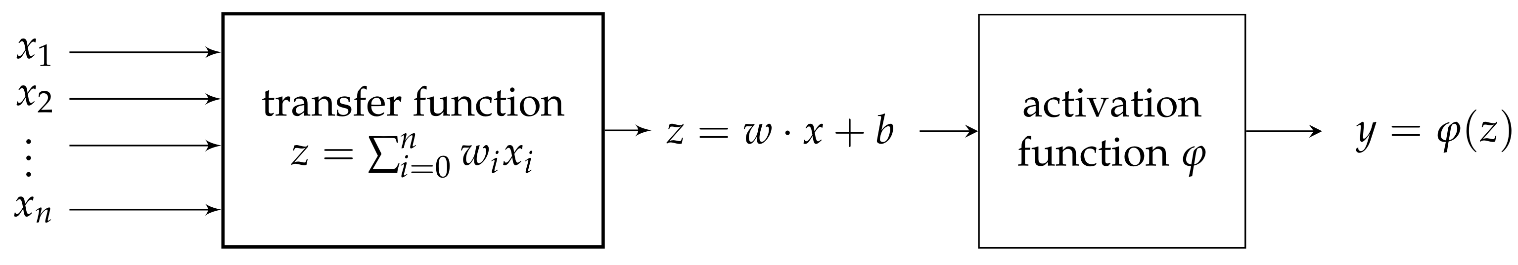
Specifically, for ANNs with just one layer (neuron), the input (that may be detailed as a vector of features ) is processed in the neuron through weights denoted by producing a z which finally results in the final output y through some function , . The whole procedure is as follows:
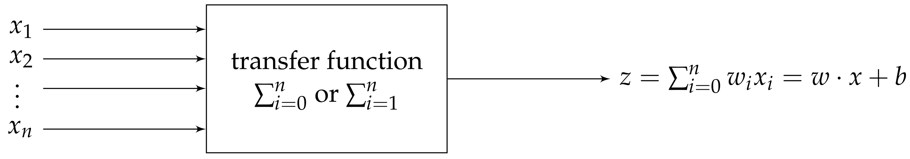
- On one hand, z is the result of processing the n-inputs throughout the weights :or by avoiding the notation for transpose, where b is called bias (the bias b is an attempt to imitate the human filter which helps to fit the given data to the real needs). This description shows this processing as an affine function . The bias may be regarded as well as a weight for an initial input , so the processing of inputs in a neuron may be seen also as a linear function:We shall freely use both perspectives—affine (1) and linear (2)—depending on needs. The processing of the n-inputs with result z is named the transfer function:Despite that the weighted sum operator is the most popular, many other alternatives may be considered as transfer functions, depending on needs.
![Axioms 11 00080 i001]()
- On the other hand, the function , which is responsible for the nonlinearity of the whole process, is known as the activation function. This may be “freely” selected as long as it meets certain requirements that we will see later.
Hence, each artificial neuron may be regarded as a mathematical function that results in an output y by chaining both the transfer function (linear) and the activation function (nonlinear) on the inputs , , see Figure 1.
For ANNs with more than one layer (MLP multilayer perceptron), let us consider the previous process as a mathematical function on the inputs: . The generalization for multilayers is simple: inputs entering a neuron become outputs after adequate processing inside (mostly, a linear combination of inputs as seen), which are sent as inputs to other neurons (the propagation of information from one layer to the next is known as feed-forward). Mathematically,
Definition 1.
A multilayer perceptron is a function. It is an n–L–m-perceptron (n inputs, L hidden layers and m outputs) if it is a function of the form
Particularly, for affine functions, one has the linear multilayer perceptron:
for, which applies a nonlinear function φ to the composition of n affine functions.
The bias has a clear geometrical meaning derived from its role in affine transformations: it measures the distance between the origin and the boundary which separates the input features.
From the viewpoint of Discrete Mathematics, an equivalent definition to Definition 1 of a multilayer perceptron is as follows:
Definition 2.
A multilayer perceptron is a directed graph with the following properties: Each node (neuron) i is associated with a state variable. Each connection between nodes i and j is associated with a weight. The value of the initial weightis known as bias. Finally, for each node i there exists a function (named the activation function). The value of this function provides the new input for the node j.
3. Theoretical Learning Algorithm
This section is aimed at unravelling the gradient descent minimum method (GDM). It is the most used methodological basis for ANN training since it significantly reduces the number of required computational calculations [15]. In addition to knowing the detail of the methodology by which the committed error is minimized to strengthen the capacity for fine-tunings, the objective of this study is to derive the necessary requirements for ANN key components, such as the activation functions.
3.1. GDM: Gradient Descent Minimum or Cauchy Descendent
The gradient descent minimum algorithm (GDM) is a first-order procedure for computing iteratively a local minimum of a differentiable function. To properly refer to this result, it must be mentioned that it was simultaneously suggested by Cauchy [10] in 1847 (hence the name “Cauchy Descendent”) and developed in a similar manner by Hadamard in 1907 [9]. A deeper analysis is attributed to Curry in 1944 [8]. In ANN literature, it is also referred to as the “Taylor expansion approach” [15]. Let us first recall the main properties of the gradient of a function of n-variables:
Theorem 1 (Gradient of a function).
Letbe a differentiable function in the neighbourhood of some point. Then, the gradient of E at, denoted,
- 1.
- represents the slope of the tangent line to the function E at the point w;
- 2.
- points in the direction in which the function E most rapidly increases; thus,indicates the direction of fastest decreasing;
- 3.
- is orthogonal to the level surfaces (generalization of the concept of a level curve for a function of two variables) of E, i.e., those of the formfor a constant k.
Then, the GDM algorithm (the most commonly used optimization algorithm for the ANNs) is as follows:
Theorem 2 (GDM algorithm).
Letbe a differentiable function. Thus, there exists a local minimum which can be reached by iteratively updating according to the dynamical system
Proof.
The aim is to update the minimum values of a given function in order to reach a local minimum. For this, let us solve the equation . An iterative procedure should be to let the function indefinitely decrease until either it vanishes or coincides with a minimum. GDM relies upon such methodology of iteratively decreasing the function in the direction stated by of fastest decreasing (see Theorem 1).
Recall that, by definition of the first derivative of a single variable function, can be approximated component-wise by approximating each of its partials as a single-variable function :
By forgetting the coordinate-wise description, thus
Let us now consider a scale factor h in the direction of fastest decreasing, for non-negative and small enough (). Thus, since both , by applying the general rule to the particular case of , one has that
where the last inequality stems from the fact that is strictly positive because both factors are. That is, the function E takes smaller values for those inputs of the form as long as remains non-negative. Recall that as before, these expressions have to be considered coordinate-wise. In the expression let us rename it as
In consequence, the sequence that updates the minimum values for a function with initial value is
for non-negative scale factors . Specifically, it is
□
Other variants of the gradient descent algorithm are the stochastic gradient descent, AdaGrad and Adam, with the same structural storyline to minimize the error [16].
3.2. Training the ANN: Updating the Weights with GDM
The process of updating the weights and biases in order to minimize the error is known as the back propagation (BP) algorithm [17]. In ML, the error function is also called the cost or loss function and the scale factor is also known as the learning rate. In overall terms, the error function measures the difference between the ANN outputs (y) and the desired values () according to several choices. One of them is Mean Square Error MSE = . In ANN literature, the Square Error is often used following the formula for cancelling the constant when computing the gradient. Other choices are Root Mean Square Error, RMSE= , Mean Bias Error, MBE= and Mean Absolute Error, MAE= (MAE ≤ RMSE.)
Let us detail now how to make use of the GDM algorithm in order to train the ANN for minimizing the error function. To this end, let us consider as an error function the Mean Square Error, , which is a function of the weight coordinates : since thus
Let us apply the chain rule for any activation function . Thus, the partial derivative is:
That is, with resulting partial derivative for the particular case of the activation function being the identity function . As for the Square Error , the resulting partial derivative is equal to
with expression , for the particular case of activation function equalling the identity function . As we shall see in Section 5, the learning algorithms for perceptrons result in particular cases of the above development for specific error functions.
The convergence of the method is ensured under suitable conditions on the error function. For this, let us review the following definition:
Definition 3.
A mapis called a Lipschitz function if there existssuch that
Particularly, when, f is called a contraction.
The class of Lipschitz functions and, particularly, contractions are absolutely continuous and, hence, differentiable almost everywhere. Recall also that a differentiable function f is said to be k-smooth if its gradient is Lipschitz continuous, that is, if there exists such that
Thus, the following theorem states conditions under the error function to assure convergence:
Theorem 3
(Convergence of gradient [18]). Suppose the function is convex, differentiable and k-smooth. Then, if we run gradient descent for r iterations with a fixed step size , it will yield a solution which satisfies
where is the minimum value. That is, the gradient descent is guaranteed to converge.
4. The Role of the Activation Function: Required Features
The best known role of activation functions is to decide whether an input should be activated or not by limiting the value of the output according to some threshold. They are mainly used to introduce nonlinearity. It should be remembered that some of the main tasks of ANNs are classification and pattern recognition. The nonlinearity of activation functions responds thus to reality, where the majority of problems have nonlinear boundaries or patterns. Another not-so-well-known role is their decision power in the success or failure of the ANN, as we shall see when exploring their determinant features regarding the applicability of the UAT. Additionally, the choice of the activation function has an important specific weight on the training process because it has a direct influence on the gradient of the error function. This section is thus devoted to exploring these contingencies as well as showing significant results that characterize/identify the best candidates for the activation function.
4.1. Derived from the Theoretical Foundations of the Training Process: First Required Properties
From the previous developments (Theorem 2 and Equations (4)–(6)), the following properties for activation functions may be derived:
Proposition 1 (Differentiability).
Activation functions should be differentiable.
Proof.
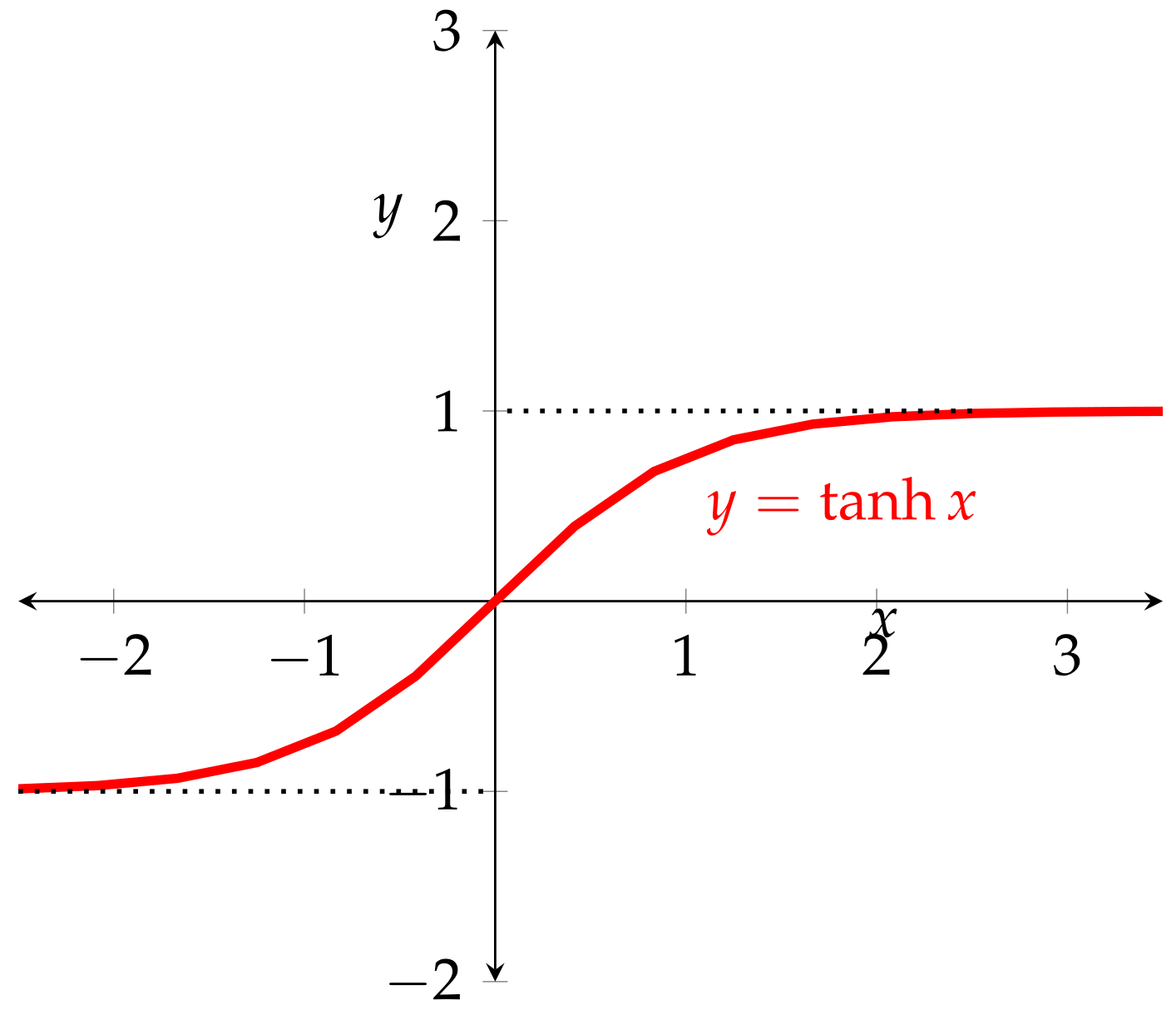
Figure 2 and Figure 3 below show instances of activation functions (characteristic/step and hyperbolic) in both contexts. The graph of the hyperbolic tangent in Figure 3 shows the characteristic S-shape of differentiable activation functions.
The previous Theorem 2 makes known that back propagation is based on minimizing the error by updating the weights at each iteration according to the Sequence (3). Hence, its efficacy strongly relies upon the stability of the direction of .
From Equation (5), it is clear that is a factor of , and the same occurs with other choices of error according to the chain rule. Thus, the stability of is conditioned by the behaviour of the first derivative of the activation function . Functions with such a good behaviour are called as follows:
Definition 4 (Gradient preserving functions).
Increasing monotonicity is highly recommended in practical guides on programming ANNs as a desired property of activation functions. Apart from ANNs’ impact on the UAT (see Section 4.3), the next proposition provides the first mathematical explanation.
Proposition 2 (Monotonically increasing/decreasing).
Monotonic functions are gradient preserving.
Proof.
From Equation (5) of the BP algorithm for the MSE Error, is a factor of . Component-wise, that is Monotonicity of assures that is either positive or negative . Hence, they are gradient preserving. □
Remark 1.
Differentiability almost everywhere. Differentiability of the activation function is not compulsory in the whole domain but only partially—as long as activation is gradient preserving. Thus, differentiability almost everywhere (i.e., to be differentiable at every point outside a set of Lebesgue measure zero) can replace differentiability as a weaker condition onto activation functions. As we shall see later (see Theorem 4), Lipschitz functions—used in designing ANN with applications in inverse problems—enjoy such a property.
Moreover, every monotonic function (increasing or decreasing) defined on an open interval (a, b) is differentiable almost everywhere on (a, b) by the Vitali covering theorem. This is (yet) another quality of monotonic activation functions that explains why they are highly used as a guarantee of ANN success.
Remark 2.
Tips from practical use. Convergence of the GDM method (Theorem 3) at a low computational cost (activation functions have to be computed millions of times in deep neural networks) highly recommends that activation functions satisfy other properties such as boundedness. While a great deal of research aimed at ensuring the stability of learning processes proposes to bound the variables (input normalization or standardization, procedures which scale the data to a range more appropriate to be processed by the ANN), some authors [11] claim the significance of using bounded activation functions in order to avoid instability. These authors proposed abounded family of well-known activation functions with results of Bounded ReLU and Bounded Leaky ReLU. Odd symmetries (called in ML zero-centred)—such as sigmoids—are also preferred in the ANN practical guides (see [19], for instance) since “they are more likely to produce outputs which are inputs to the next layer that are on average close to zero” [19].
4.2. Influence of Activation Functions on the Training Process
As mentioned, for the nature of the Sequence (3) in Theorem 2, it is clear that the effectiveness of updating the weights will depend on whether the direction of remains stable. Otherwise, the convergence of the GDM could be compromised or it could even be achieved at a high computational cost if the process slows down. In ANN literature, this is known as the vanishing gradient problem, or VGP. Instability in the convergence of the learning method would appear if, after r iterations in the BP algorithm, the gradient vector tended to the zero vector, denoted by
Additionally, by interpreting the first derivative as a rate of change, after r iterations implies that the velocity of error tends to diminish and may end.
The following developments are intended to identify gradient preserving activation functions. The following proposition includes in its proof detailed information on the back propagation procedure in order to obtain conditions on the activation functions. It is also intended to introduce the next main theorems (and shorten proofs):
Proposition 3.
Letbe a differentiable function such that. Then, φ is a contraction that satisfies.
Proof.
First, note that the first statement is equivalent to either or . First, we prove that
By Equation (5),
Hence, after r iterations of the BP algorithm (corresponding to an ANN with r layers),
where denotes the resulting vector after r iterations. According to the property for potential functions such that , the factor in verifies
The Riemann integral preserves inequalities; hence, the inequality holds with respect to z:
Let us remember that, however, differentiation does not preserve inequalities. In order to prove that is a contraction (see Definition 3) we refer to the Lagrange mean value theorem. Thus, as is continuous over and differentiable over (since it is differentiable on ),
Then, , where .
Hence, is a contraction. □
This in-depth study of ANN structures and properties of the activation functions shall lead us to useful characterizations of those with better behaviour regarding GDM (gradient preserving functions according to Definition 4). The next theorems thus gather this information.
Theorem 4.
For any nonconstant monotonically increasing function, the following statements are equivalent:
- 1.
- .
- 2.
- φ is a contraction.
Proof.
First, let us note that, according to Remark 1, both monotonically increasing and contraction mappings are differentiable almost everywhere. In addition, note that to be a nonconstant monotonically increasing function on is equivalent to , since implies is constant.
The implication has been shown in the previous Proposition 3.
Let us prove the converse . For this, we use the definition of the first derivative:
where
Hence, since is a contraction. Thus
Theorem 4 is used in its contrapositive form: while contractions and related mappings which satisfy the classical contractive condition are not gradient preserving, Lipschitz functions are. Specifically, the next theorem provides a characterization of gradient preserving activation functions (as Lipschitz but not contractive):
Theorem 5 (Characterization of gradient preserving activation functions).
For any differentiable nonconstant function , the following are equivalent:
- (i)
- φ is gradient preserving.
- (ii)
- such that .
- (iii)
- φ is a Lipschitz function of constant k.
Proof.
Let us suppose that such that and consider . According to the Lagrange mean value theorem,
φ is a Lipschitz function of constant k. Conversely, for , consider
□
4.3. Influence of Activation Functions on Applicability of Universal Approximation Theorem: Injectivity
In this section, we explore the properties of activation functions with regard to ANNs as universal approximators of continuous functions. Amongst the different formulations of the classical Universal Approximation Theorem (e.g., [1,2,3]), we select the one from [20], where the activation function has been identified with the whole neural network, thereby stressing its importance:
Theorem 6
(UAT, [20]). For any and continuous function f on a compact subset , there is a neural network with activation function φ with a single hidden layer containing a finite number n of neurons that, under mild assumptions on the activation function, can approximate f, i.e.,
Since then, several approaches have been provided by addressing extensions for larger ANN architecture (e.g., multiple layers or multiple neurons).
We shall focus on injectivity as the desired property for activation functions because it plays a key role regarding the following issues: Firstly, injectivity is determinant for those ANNs which require inversion on their range. That means that, given a neural network (from Definition 1, this is of the form ), the map
is well-defined only when F is injective. In such contexts, such as reconstruction problems—image retrieval, for instance—it is compulsory that multiple outputs (F(x) = F(y)) come from a unique input, . Secondly, injectivity has key implications on the universal approximator capabilities of ANNs. Thirdly, injectivity (and more) over an activation function may imply stability in the GDM learning algorithm through the strict monotonicity which may be derived from injectivity (see Theorem 7).
Regarding the first issue, the following proposition shows that the ANN inherits injectivity if the activation function is injective:
Proposition 4.
Let be a multilayer perceptron as given in Definition 1. The activation function φ is injective ⇒ F is injective.
Proof.
According to Definition 1, the multilayer perceptron is
Hence, F is a composition of injective maps, since affine functions are. By consequence, F is injective. □
Let us address the second issue (UAT). To ensure that the Universal Approximation Theorem holds for some architecture of ANNs, there are some specifications on the activation function to be met: to be a nonconstant function, nonpolynomial, bounded within a range of values (see also Remark 2) continuous on their domain, continuously differentiable at least one point and monotonically increasing. Importantly, while monotonicity of activation functions, either increasing or decreasing, reinforces the convergence of the GDM algorithm, only increasing monotonicity is required for activation functions regarding the UAT.
As for injectivity regarding the UAT, we refer to work [21], where a particular case of continuous activation functions are introduced, those which satisfy any of the following equivalent conditions: is injective and has no fixed points ⇔ either or holds for every . In that paper, it is shown that activation functions which satisfy one of the previous equivalent conditions allow us to ensure that a kind of neural network (with a particular architecture) meets the UAT.
As for the third issue, the following theorem is a characterization of injectivity (and more) in terms of strict monotonicity, thereby providing a further mathematical explanation of the level of importance given in the practical use of ANNs to increasing/decreasing activation functions (apart from being gradient preserving; see Section 4.1, Theorem 2 and Section 4.2):
Theorem 7 (Characterization of injectivity with no fixed points).
Let be any real-valued function. Thus, the following statements are equivalent:
- (i)
- φ is strictly monotonic.
- (ii)
- φ is injective with no fixed points.
Proof.
Let be a strictly monotonic function, either increasing or decreasing. Let us show that it is injective. For this, let us suppose that and . Thus, there are two options: or . In the first case, the monotonicity of the function implies that if increasing or if decreasing. Similarly, for the second case, we also reach a contradiction. Thus, . Note that strictness does not allow the existence of fixed points. Conversely, let be injective with no fixed points and suppose that . Thus, regarding and , they cannot be equal (). In consequence, either or . That concludes the proof. □
Remark 3.
By combining the previous Theorem 7 with the stated result of [21] and the well-known characterization of monotonicity in terms of the sign of the first derivative, strictly monotonic activation functions (easily identifiable by checking the sign of their first derivatives) characterize the UAT for a particular type of ANNs.
4.4. Mainly Used Activation Functions
There are several categorizations of activation functions. Instead of stressing the criteria of classification, we shall display the most commonly used together with their main properties (see Table 1). Following [22], we shall focus on “fixed-shape activation functions” which are activation functions with no hyperparameters to be altered during the training. These are divided into classic activation functions (step, sigmoidal and hyperbolic tangent) and those which belong to the family of ReLU functions (the function ReLU was firstly introduced by [23]; see also [24] for an empirical proof that the ReLu function improves the learning process).
5. Practical Learning Algorithm
As is known, perceptrons are artificial neural networks consisting of one single neuron and two layers, input and output. This also refers to simple computational models consisting solely of a neuron. They are fruitful in contexts where there are only two different features to be disassociated. That is, as linear classification models, they are able to accurately classify as long as the classes are linearly separable (i.e., the set of features may be divided by a line, plane or hyperplane). In this section, we shall see how the practical algorithm of the perceptron works in complete concordance with the theoretical results exposed throughout the paper.
The practical training ANN code is:
- n represents the time step (days, weeks, etc.)
- In the 0th step, consider the input vector (and its classification, so ) and the weights vector .
- Compute .
- Compute .
- Compare with . Update in consequence the weight (if necessary) for the next step.
- With the same input in the next time step , repeat all.
- Stop when there are no wrongly classified.
Let us suppose that there are the two classes, 1 and 2, that are are linearly separable. Then, there exists a vector of weights w such that it meets the following expressions: for each input vector x that belongs to class 1 and for each input vector x that belongs to class 2. Given the training subsets and (with vectors which belong to the two different classes, respectively), the training problem of the elementary (two-layer) perceptron is then to find a vector of weights that satisfies the previous two inequalities. Note that the line, plane or hyperplane linearly separates the inputs when it is or .
The functioning of this practical algorithm is:
- If the nth element of the training vector (we knew in advance what class belonged to) is accurately classified by the vector of weights calculated in the nth iteration of the algorithm, no rectification of the perceptron weight vector is performed, i.e.,
- Otherwise (when the training vector is wrongly classified), the weight vector of the perceptron is updated according to the following rule:for equal to a sign: positive if the outcome and the desired result are equal (and, hence, the classification has been well performed) and negative otherwise:
The learning algorithm is as follows:
- Variables and parameters:
The stages of the learning algorithm are:
- Step 1: initialization We make , and the following calculations are carried out in the instants of time
- Step 2: activationThe perceptron is activated throughout and as follows:i.e., the desired response expresses whether the classification of is well performed.
- Step 3: calculation of the current answer (output) The current response of the perceptron is computed:
- Step 4: adaptation of the weight vectorLet us remember that and are equal when the classification is well performed. In the affirmative case, and , as stated before.
- Step 5: Increase n by one and go back to step 2.
6. Conclusions
Artificial Neural Networks are very successful tools in a wide range of problems involving classification/pattern recognition, regression or forecasting. The core of this success is the quality of ANNs being universal approximators of continuous functions (UAT), a line of research that began in 1989 and that reappears today to provide mathematical arguments in response to the good performance of the ANNs.
This paper is intended for supporting with mathematical arguments all those recommendations derived from ANN practical usage that are widely accepted. This is the case, for instance, with those useful tips that are usually exchanged in the context of networking software, which is mainly based on the exhibited behaviour in practice of the ANN components (e.g., zero-centred, differentiable, computationally inexpensive and “good performance as for the GDM”, which are the most commonly recommended properties for activation functions). In this work, through an in-depth study of ANN structures and properties of activation functions, useful characterizations of those with better behaviour are provided. Alongside such analysis, a list of required properties of activation functions has been built: to be a nonconstant function, to be a nonpolynomial, to be bounded within a range of values, to be odd symmetrical, to be differentiable, to be continuously differentiable at at least one point, to be differentiable almost everywhere, to be monotonic either increasing or decreasing and to be Lipschitz.
In addition, injectivity is a quality less known than those stated previously but with strong implications regarding the potential performance of ANNs. Moreover, to be injective with no fixed points has significant effects. For the enhancement of the stability of the training method, it has been also proved that while Lipschitz functions are good choices, contractions must be avoided to guarantee good behaviour in preserving the direction of the gradient vector.
In the future, this list of specifications will be supplemented by the requirements on the activation functions in the field of real-life application.
Funding
This research received no external funding.
Acknowledgments
Financial support from the Spanish Ministry of Universities. “Disruptive group decision making systems in fuzzy context: Applications in smart energy and people analytics” (PID2019-103880RB-I00). Main Investigator: Enrique Herrera Viedma, and Junta de Andalucía. “Excellence Groups” (P12.SEJ.2463) and Junta de Andalucía (SEJ340) are gratefully acknowledged. Research partially supported by the “Maria de Maeztu” Excellence Unit IMAG, reference CEX2020-001105-M, funded by MCIN/AEI/10.13039/501100011033/.
Conflicts of Interest
The authors declare no conflict of interest.
References
- Cybenko, G. Approximation by superpositions of a sigmoidal function. Math. Control Signals Syst. (MCSS) 1989, 2, 303–314. [Google Scholar] [CrossRef]
- Hornik, K. Approximation capabilities of multilayer feedforward networks. Neural Netw. 1991, 4, 251–257. [Google Scholar] [CrossRef]
- Hornik, K.; Stinchcombe, M.; White, H. Multilayer feedforward networks are universal approximators. J. Neural Netw. 1989, 2, 359–366. [Google Scholar] [CrossRef]
- Hanin, B. Universal Function Approximation by Deep Neural Nets with Bounded Width and ReLU Activations. Mathematics 2019, 7, 992. [Google Scholar] [CrossRef] [Green Version]
- Kidger, P.; Lyons, T. Universal Approximation with Deep Narrow Networks. In Proceedings of the Thirty Third Conference on Learning Theory, Graz, Austria, 9–12 July 2020; Volume 125, pp. 2306–2327. [Google Scholar]
- Moon, S. ReLU Network with BoundedWidth Is a Universal Approximator in View of an Approximate Identity. Appl. Sci. 2021, 11, 427. [Google Scholar] [CrossRef]
- Cooper, S. Neural Networks: A Practical Guide for Understanding and Programming Neural Networks and Useful Insights for Inspiring Reinvention; Data Science, CreateSpace Independent Publishing Platform: Scotts Valley, CA, USA, 2019. [Google Scholar]
- Curry, H.B. The Method of Steepest Descent for Non-linear Minimization Problems. Q. Appl. Math. 1944, 2, 258–261. [Google Scholar] [CrossRef] [Green Version]
- Hadamard, J. Memoire sur le Probleme D’analyse Relatif a Vequilibre des Plaques Elastiques Encastrees; L’Academie des Sciences de l’Institut de France: Paris, France, 1908; Volume 2, p. 4. [Google Scholar]
- Lemarechal, C. Cauchy and the Gradient Method. Doc. Math. Extra 2012, 251, 10. [Google Scholar]
- Liew, S.; Khalil-Hani, M.; Bakhteri, R. Bounded activation functions for enhanced training stability of deep neural networks on visual pattern recognition problems. Neurocomputing 2016, 216, 718–734. [Google Scholar] [CrossRef]
- Fiesler, E. Neural network classification and formalization. Comput. Stand. Interfaces 1994, 16, 231–239. [Google Scholar] [CrossRef]
- Popoviciu, N.; Baicu, F. The Mathematical Foundation and a Step by Step Description for 17 Algorithms on Artificial Neural Networks. In Proceedings of the 9th WSEAS International Conference on AI Knowledge Engineering and Data Bases, Cambridge, UK, 20–22 February 2010; p. 23. [Google Scholar]
- Kreinovich, V. From Traditional Neural Networks to Deep Learning: Towards Mathematical Foundations of Empirical Successes. In Recent Developments and the New Direction in Soft-Computing Foundations and Applications. Studies in Fuzziness and Soft Computing; Springer: Cham, Switerland, 2021; pp. 387–397. [Google Scholar] [CrossRef]
- Cooper, A.M.; Kastner, J.; Urban, A. Efficient training of ANN potentials by including atomic forces via Taylor expansion and application to water and a transition-metal oxide. Comput. Mater. 2020, 6, 54. [Google Scholar] [CrossRef]
- Duchi, J.; Hazan, E.; Singer, Y. Adaptive Subgradient Methods for Online Learning and Stochastic Optimization. J. Mach. Learn. Res. 2011, 12, 2121–2159. [Google Scholar]
- Cun, Y.L.; Boser, B.; Denker, J.S.; Henderson, D.; Howard, R.; Hubbard, W.; Jackel, L. Handwritten digit recognition with a back-propagation network. Adv. Neural Inf. Process. Syst. 1990, 2, 396–404. [Google Scholar]
- Zhang, L.; Zhou, Z.H. Stochastic Approximation of Smooth and Strongly Convex Functions: Beyond the O(1/T) Convergence Rate. In Proceedings of the Thirty-Second Conference on Learning Theory, Phoenix, AZ, USA, 25–28 June 2019; PMLR 99. pp. 3160–3179. [Google Scholar]
- Orr, B.G.; Muller, K.L. Neural Networks: Tricks of the Trade; Springer Lecture notes in Computer Science; Springer: Berlin/Heidelberg, Germany, 1998; p. 1524. ISBN 3-540-65311-2. [Google Scholar]
- Leshno, M.; Lin, V.Y.; Pinkus, A.; Schocken, S. Multilayer feedforward networks with a nonpolynomial activation function can approximate any function. Neural Netw. 1993, 6, 861–867. [Google Scholar] [CrossRef] [Green Version]
- Kratsios, A. The Universal Approximation Property. Characterization, Construction, Representation, and Existence. Ann. Math. Artif. Intell. 2021, 89, 435–469. [Google Scholar] [CrossRef]
- Apicella, A.; Donnarumma, F.; Isgro, F.; Prevete, R. A survey on modern trainable activation functions. Neural Netw. 2021, 138, 14–32. [Google Scholar] [CrossRef] [PubMed]
- Nair, V.; Hinton, G.E. Rectified linear units improve restricted Boltzmann machines. In Proceedings of the 27th International Conference on Machine Learning, (ICML10), Haifa, Israel, 21–24 June 2010; pp. 807–814. [Google Scholar]
- Kazuyuki, H.; Daisuke, S.; Hayaru, S. Analysis of function of rectified linear unit used in deep learning. In Proceedings of the 2015 International Joint Conference on Neural Networks (IJCNN), Killarney, Ireland, 12–17 July 2015; IEEE: Piscataway, NJ, USA, 2015; pp. 1–8. [Google Scholar]
Figure 1.
Single artificial neuron functioning.

Figure 2.
Step function (not differentiable).
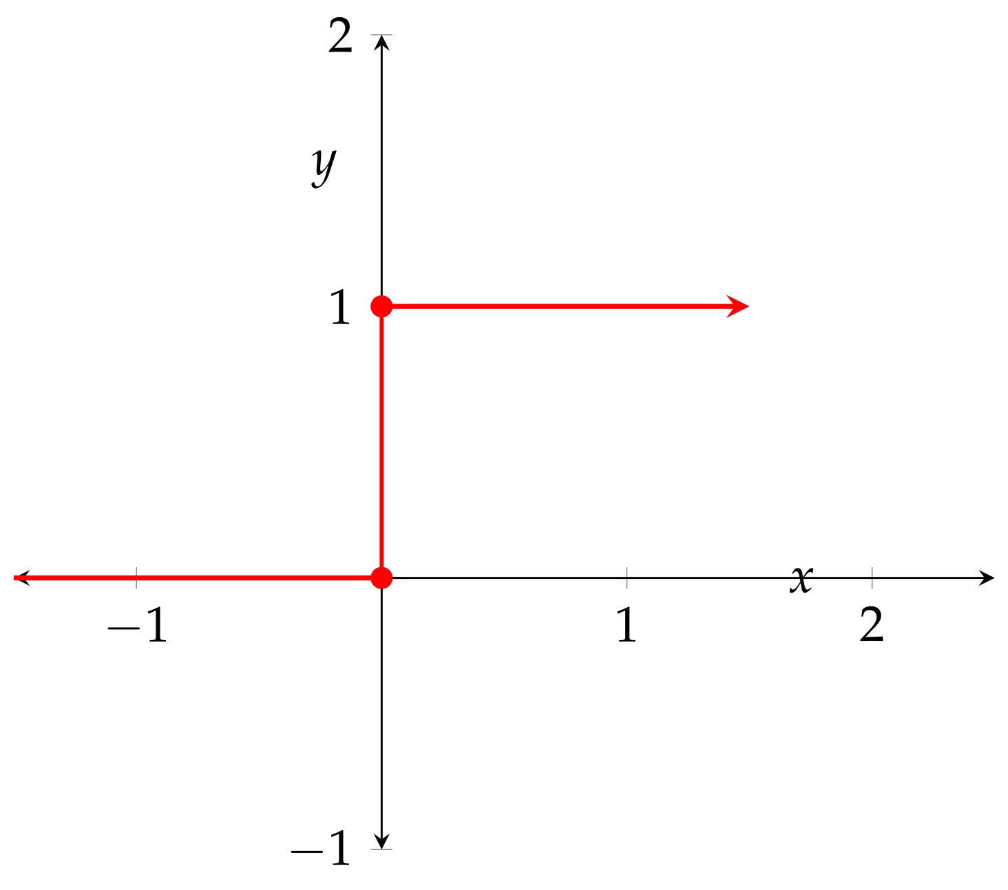
Figure 3.
Hyperbolic function (differentiable).

Table 1.
Practical Learning Algorithm.
| Name | Mathematical Expression | Properties | |
|---|---|---|---|
| Discrete | Step function (or threshold) |
| |
| ReLU (Rectified Linear Unit) |
| ||
| Leaky ReLU |
| ||
| Continuous | Sigmoidal |
| |
| Hyperbolic tangent |
| ||
Publisher’s Note: MDPI stays neutral with regard to jurisdictional claims in published maps and institutional affiliations. |
© 2022 by the author. Licensee MDPI, Basel, Switzerland. This article is an open access article distributed under the terms and conditions of the Creative Commons Attribution (CC BY) license (https://creativecommons.org/licenses/by/4.0/).
Share and Cite
MDPI and ACS Style
García Cabello, J. Mathematical Neural Networks. Axioms 2022, 11, 80. https://doi.org/10.3390/axioms11020080
AMA Style
García Cabello J. Mathematical Neural Networks. Axioms. 2022; 11(2):80. https://doi.org/10.3390/axioms11020080
Chicago/Turabian StyleGarcía Cabello, Julia. 2022. "Mathematical Neural Networks" Axioms 11, no. 2: 80. https://doi.org/10.3390/axioms11020080
APA StyleGarcía Cabello, J. (2022). Mathematical Neural Networks. Axioms, 11(2), 80. https://doi.org/10.3390/axioms11020080
Note that from the first issue of 2016, this journal uses article numbers instead of page numbers. See further details here.