Logarithmic SAT Solution with Membrane Computing

Abstract

P systems have been known to provide efficient polynomial (often linear) deterministic solutions to hard problems. In particular, cP systems have been shown to provide very crisp and efficient solutions to such problems, which are typically linear with small coefficients. Building on a recent result by Henderson et al., which solves SAT in square-root-sublinear time, this paper proposes an orders-of-magnitude-faster solution, running in logarithmic time, and using a small fixed-sized alphabet and ruleset (25 rules). To the best of our knowledge, this is the fastest deterministic solution across all extant P system variants. Like all other cP solutions, it is a complete solution that is not a member of a uniform family (and thus does not require any preprocessing). Consequently, according to another reduction result by Henderson et al., cP systems can also solve k-colouring and several other NP-complete problems in logarithmic time.

1. Introduction

The P-versus-NP problem remains one of the most important unsolved problems in computational complexity theory. Loosely following Sipser [1] and keeping the discussion focused on deterministic algorithms—as we do throughout this paper—the class P can be viewed as the class of decision problems that can be solved “quickly”, whereas NP can be viewed as the possibly larger class of decision problems with solutions that can be verified “quickly”, where “quickly” is taken in the theoretical sense, i.e., polynomial time. It is straightforward to see that P ⊆ NP. However, it is still unknown whether this inclusion is strict or not, in other words, whether P ⊊ NP or P = NP. In a nutshell, the big theoretical question is whether every problem of which the solution can be verified in polynomial time (NP) can also be solved in polynomial time (P).

The current widespread opinion is that P ⊊ NP, as there are quite a few “hard” problems that can be “quickly” verified, but do not seem to have “quick” solutions, with their fastest known solutions taking time substantially greater than any polynomial (e.g., exponential). Therefore, many studies have investigated different approaches to solve such hard problems in a reasonable amount of time (e.g., polynomial or even linear time). Such methods include approximation [2], fixing parameters [3], or the use of alternative theoretical models, such as P systems [4,5,6,7,8,9].

P systems—also known as membrane computing—are a family of parallel and distributed biologically inspired models of computing, proposed by Gheorghe Păun in [10], first as cell-like P systems, then followed by many variants, such as P systems with active membranes [11], tissue-like P systems [12], neural-like P systems [13], and P systems with compound terms (cP systems) [14,15]. These systems have been found to have theoretically time-efficient solutions to many hard problems, even beyond NP, e.g., in PSPACE [16,17,18,19,20,21].

It may be worthwhile to note that, with the exception of cP systems, most other P systems solutions are actually uniform families of related solutions, with one custom solution (e.g., custom alphabet and ruleset) for each problem size n. Here, uniform means that each custom size n solution is built via an additional preprocessing phase, by means of an ad-hoc polynomial-time algorithm (typically not described but reasonably evident). In contrast, cP solutions are given by fixed-size alphabets and rulesets (typically small), while running with the same theoretical efficiency, or even faster.

In this work, we present a novel deterministic cP solution to SAT, running in logarithmic time, $\mathcal{O}(logn)$. To the best of our knowledge, this represents a significant breakthrough in membrane computing, being orders-of-magnitude faster than all previous deterministic solutions. As mentioned, we do not consider here the interesting area of non-deterministic computations, where there are several interesting results, e.g., using neural-like P systems [22].

Our novel solution builds upon and substantially improves the already very fast cP solution to SAT recently proposed by Henderson et al. [4], which runs in square-root time, $\mathcal{O}\left(\sqrt{n}\right)$. The solution presented here is based on a fast method of creating and evaluating a complete binary tree of height n, in $\mathcal{O}(logn)$ time. When measuring the number of rule templates, we see that our new solution is comparable to those of previous P systems studies. However, when counting rules rather than the templates, we see that other solutions can have an exponential number of rules.

Using the results presented in this paper, reductions such as those presented in Stamm-Wilbrandt [23] and Henderson et al. [4] will enable more logarithmic time solutions, $\mathcal{O}(logn)$, to quite a few other NP-complete problems, such as k-colouring.

However, to the best of our knowledge, all these efficient solutions are still theoretical and have not yet been practically implemented. Designing efficient, practical implementations is a topic of current research.

2. Background

In this section, we briefly recall the well-known Boolean satisfiability problem (SAT) and we offer a short introduction to cP systems.

2.1. The SAT Problem

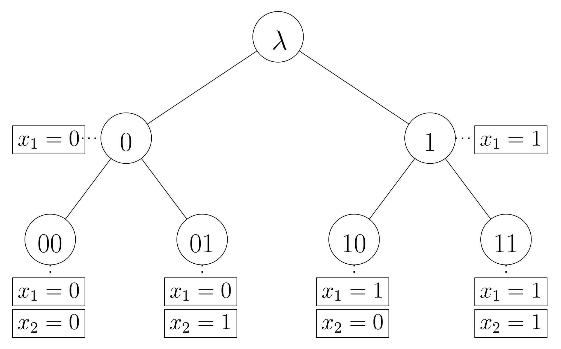
SAT is one of the best-known examples of an NP-complete problem and is a relatively simple but central problem in many areas of computer science (e.g., complexity, artificial intelligence, cryptography, etc.). Like all other NP-complete problems, it has no known (worst-case) polynomial solution in the Turing machine model (or related models). In this paper, we show that cP systems can theoretically solve SAT in sublinear logarithmic time.

SAT determines if the variables of a given Boolean formula can be assigned Boolean values that evaluate the formula to true. A Boolean formula is an expression involving Boolean variables and Boolean operations. A Boolean formula is in conjunctive normal form (CNF) if it is expressed as a conjunction (∧) of clauses. A clause is a disjunction (∨) of literals. A literal is a variable or its negation (here indicated by overbars).

Basic SAT assumes that the formulae are given in CNF, with implicit existential quantifiers on all variables. The existential quantifier (∃) results are true if one of the possible assignments of the variables allows the formula to be true.

Example 1.

For example, the following Boolean formula with two variables is in CNF:

$(x_1\vee x_2)\wedge (\overline{x_1}\vee \overline{x_2})$.

SAT interprets the above formula as the following decision problem:

$\exists x_1\exists x_2(x_1\vee x_2)\wedge (\overline{x_1}\vee \overline{x_2})$.

The size of the problem is given by the number of variables, n, e.g., $n=2$, for the formula of Example 1. There are straightforward bijections between several sets of size $2^n$: (i) candidate solutions (variable allocations) of a CNF formula with n variables, (ii) (characteristic functions for) subsets of set $\{1,2,\dots ,n\}$, (iii) branches (root-to-leaf paths) of the complete binary tree of height n. For case (iii), a tree path starting from a root can be naturally labelled as a string of bits, where bits indicates its left/right “choices” (turns) in the top-down (root-to-leaf) order.

Example 2.

Consider the complete binary tree of Figure 1 of height $n=2$, with 4 branches, in left-to-right order:

Branch	SectionAllocations	Subset
00	$x_1=0,x_2=0$	$\left\{\right\}\left(empty\right)$
01	$x_1=0,x_2=1$	{ 2 }
10	$x_1=1,x_2=0$	{ 1 }
11	$x_1=1,x_2=1$	{ 1, 2 }

Note that branches 01 and 10 correspond to solutions for the formula of Example 1.

Our cP solution is based on a parallel construction of complete binary tree branches, followed by a parallel formula evaluation on these branches.

2.2. cP Systems

In this paper we propose a novel cP solution to a hard problem; to the best of our knowledge, this is the first P solution running in logarithmic time, which represents an improvement of orders of magnitude.

P systems, also known as membrane computing, are a framework for designing computational models inspired by biology. Similarly to many other P systems variants, such as cell-like and tissue-like P systems, cP systems are based on nested labelled multisets and offer: (i) unbounded access to resources, such as space and processing power; (ii) top-level cells, with sub-cells organised into nested tree structures; (iii) graph based networks of top-level cells; and (iv) evolutions driven by formal multiset rewriting rules, with additional messaging primitives between top-level cells.

However, distinctively, cP systems’ multiset rewriting rules are generic, with variables instantiated by one-way unification (pattern matching). In conjunction with nesting, generic rules provide useful logical and associative capabilities, including good support for emulating arithmetic with natural numbers (base one) and usual data structures (such as lists, strings, and associative arrays). Recall that instantiations assign values to variables—ground values in pattern matching—whereas unifications are matching instantiations.

Leveraging their capabilities, most P systems variants, including cP systems, are able to transform “brute-force” algorithms into theoretically efficient solutions, with typically linear or sublinear runtimes. This allows the design of theoretically fast solutions to hard problems. Moreover, cP systems solutions for hard problems are typically the fastest, having small runtime coefficients. Additionally, cP systems solutions typically use small rulesets of fixed sizes, which do not change with the problem size (no uniform families, no polynomial preprocessing).

In this section, we introduce the basic features of a simplified version of cP systems, called single-cell cP systems, which have one single top-level cell, with nested sub-cells (thus there is no place for top-level cell networks and messaging). Listing 1 describes the basic formal syntax of single-cell cP-systems; for a more comprehensive description and explanation of cP systems, the reader is referred to [14,15]. This formal description consists of two BNF-like grammars, presented together, because of their similarities: (1) a top-level cell, in the sequel called top-cell (for brevity); (2) a multiset rewriting rule. Note that, in this figure and the sequel, we use the following two common abbreviations: lhs = left-hand-side, rhs = right-hand-side.

Listing 1. Simplified syntax for single-cell cP systems. Lhs = left-hand-side, rhs = right-hand-side, var-X = X may contain variables. Braces ({,}) and brackets ([,]) are meta-syntactic constructs followed by repetition bounds; here, braces generate multisets, whereas brackets generate sequences.

<top-cell> ::= <state> <objects> <state> ::= <atom> <objects> ::= {<atom> | <sub-cell>}${}_0^{\infty }$ <sub-cell> ::= <functor> ’(’<objects> [’;’ <objects>]${}_0^{\infty }$ ’)’ <functor> ::= <atom> ................................................................................................................................................ <rule> ::= <lhs> ${\to }_{<}\mathrm{mode}>$ <rhs> [’|’ <promoters>]${}_0^{\infty }$ <mode> ::= ’1’ | ’+’ <lhs> ::= <state> <var-objects> <rhs> ::= <state> <var-objects> <state> ::= <atom> <promoters> ::= <var-objects> <var-objects> ::= {<variable> | <atom> | <var-sub-cell>}${}_0^{\infty }$ <var-sub-cell> ::= <functor> ’(’<var-objects> [’;’ <var-objects>]${}_0^{\infty }$ ’)’ <functor> ::= <atom>

A single-cell cP system consists of one single top-cell, which—following the first grammar presented in Listing 1—has a state and contains objects, i.e., atoms and recursively nested sub-cells.

Remark 1.

In Prolog terminology, cell objects are terms, sub-cells are compound terms; and all cell objects are ground, i.e., cannot contain variables. Furthermore, unlike Prolog, cP functors do not have arities, and just represent multiset labels.

Conventionally, atoms are represented by lowercase letters and variables by uppercase letters. A dedicated atom 1 is typically used to represent unary natural numbers (more details below). Anonymous (discard) variables in cP systems are denoted by underscores ($\underline{}$). The empty multiset is denoted by $\lambda$. As usual, multiset elements can be written in any order, and repetitions can be denoted as powers. Sample ground sub-cells: $a\left(bbc\right)=a\left(b^{2}c\right)=a\left(bcb\right)$, $a\left(b\right(cc\left)d\right(ef\left)\right)$, $n\left(\mathit{\text{111}}\right)=n\left({\mathit{\text{1}}}^3\right)$.

Remark 2.

The grammar given in Listing 1 specifies that a sub-cell functor can be followed by a sequence of multiset arguments, which seems to require an ad hoc ordering concept. Functors with one single multiset argument are indeed essential in cP systems (similar to terms in Prolog), but functors with two or more arguments are not, because these could be replaced by one more level deeper cell nesting. For example, the sub-cell $a(bc;de;fg)$ could be also considered a shorthand for $a(bc·(de):(fg\left)\right)$ (or $a(:(fg)bc·(de\left)\right)$, etc.), where the nested functors (·) and (:) could be given ad hoc or provided by the system. Briefly, this conceptually redundant ordering appears for convenience only, and the given grammar could be simplified, and strictly restricted to nested labelled multisets. Note that alternative definitions of cP systems use additional parentheses instead of the semicolons used here, e.g., the following two notations describe the same abstract syntax $a(bc;de;fg)\equiv a\left(bc\right)\left(de\right)\left(fg\right)$.

As mentioned, natural numbers can be emulated using a dedicated unary symbol, such as 1. By convention, we can also directly use the corresponding numbers, rather than their lower-level unary representation. For example:

$\mathit{111}={\mathit{\text{1}}}^3=3$

$\lambda ={\mathit{\text{1}}}^0=0$

A single-cell cP system evolves through a sequence of configurations by changing its state and contents. These changes are driven by the high-level rewriting rules associated to its top-cell, which are constructed according to the second grammar presented in Listing 1. Unlike similar cells in cell-like P systems, cP sub-cells are more restricted, by not having their own rules. Thus, sub-cells are just data storage facilities, and are acted upon by the top-cell’s rules only. This restriction seems substantially outweighed by the extra power of the cP rules. Unlike other P systems variants, rules in cP systems are generic templates, i.e., their var-objects may contain variables that must be instantiated before the rule application.

Before a rule can apply:

• Its lhs state must match the current top-cell state.
• Its rhs state must match the already committed next state, if any, as further detailed below, in the section on weak priority order.
• The rule must be completely instantiated, i.e., all its variables must be replaced by ground objects, ensuring that its lhs and promoter var-objects match extant top-cell objects.

Rules are applied in a weak priority order, with rules considered in the given top-down order. Conventionally, the first lhs state is the state of the initial configuration. Once an applicable rule has been found, this commits to the next state, with subsequent rules committing to different states disabled. Rules going to the same state as the applicable rule, which can also be applied, will be applied in the same step. This state-based weak priority order supports a straightforward emulation of basic control flow (e.g., goto, conditional goto, or loop structures). Note that rules can be partitioned by their lhs state, without altering the semantics, as long as we keep the relative top-down order of rules starting with the same lhs state.

Essentially, applying a rule:

• Commits to the next state.
• Consumes (deletes) extant top-cell objects matching its lhs. Promoters must also match extant top-cell objects, but are not consumed by the rule.
• Creates new objects as indicated by its instantiated rhs. Newly created objects are temporary unavailable and become available after the end of the current step only, as in traditional P systems.

There are two rule application modes: exactly-once (${\to }_1$) and max-parallel (${\to }_{+}$). An exactly-once rule will apply for one single matching (non-deterministically chosen). A max-parallel rule will apply it as many times as possible, conceptually all in the same step, but following a serialisation semantics, i.e., its effects must be identical to a sequential repetition of the same rule in the exactly-once mode (sequence non-deterministically chosen). Although, as just mentioned, the cP semantics allow non-deterministic computations, most of our work has focused on confluent evolutions, often deterministic; the solution proposed in this paper is deterministic.

As with most other P system variants, the runtime of single-cell cP systems is measured in steps. Generally, a step is indicated by a state change, when a rule commits to a rhs state that differs from its lhs state. If the last applied rule does not change the state, then the control resumes at the first rule of that state, and this is also counted as a step. The system halts if a rule commits to a state with no associated rule; such states are called final. The system also halts if there are rules for the current state, but none is applicable (†). This last case, marked by a dagger (†), can be easily avoided by adding an extra catch-all rule, which will ensure termination in final states only.

As mentioned, like many other P system rules, cP rules have a significant potential for non-determinism. However, well-designed practical applications are highly deterministic. A cP system is rule-deterministic if each rule ends with exactly the same results, regardless of whether it is exactly-once or max-parallel, or how exactly it is instantiated and executed. A cP system is step-deterministic if each step is locally confluent with a guaranteed join after all step rules are applied, i.e., the step ends with exactly the same result, regardless of how its rules are applied. Obviously, rule-determinism is the stronger version, implying the weaker version, step-determinism. In both cases, we consider only evolutions that start from an expected initial configuration (not from arbitrary contents).

2.3. Examples

We provide several examples to clarify how cP systems are defined and used.

Example 3.

Matching examples, var-object (left) = ground object (right):

• Matching $a\left(b\left(X\right)c\left(1X\right)\right)=a\left(b\left({\mathit{\text{1}}}^2\right)c\left({\mathit{\text{1}}}^3\right)\right)$ deterministically instantiates one single unifier: $X={\mathit{\text{1}}}^2$.
• Matching $a\left(b\left(X\right)c\left(\mathit{\text{1}}X\right)\right)=a\left(b\left({\mathit{\text{1}}}^2\right)c\left({\mathit{\text{1}}}^2\right)\right)$ fails.
• Matching $a\left(X{Y}^2\right)=a\left(d{e}^{2}f\right)$ deterministically instantiates one single set of unifiers: $X,Y=df,e$.
• Matching $a\left(XY\right)=a\left(df\right)$ non-deterministically instantiates one of the following four sets of unifiers: $X,Y=\lambda ,df$; $X,Y=df,\lambda$; $X,Y=d,f$; $X,Y=f,d$.

Example 4.

Consider a cell in state $s_1$ that contains two objects $a\left(\mathit{\text{1}}\right)$, $a\left(\mathit{\text{11}}\right)$. Depending on the actual application mode $\alpha \in \{1,+\}$, the following rule increments one or both a’s by 1:

$s_{1}a\left(X\right){\to }_{\alpha }{s}_{2}a\left(\mathit{\text{1}}X\right)$

By unifying the lhs $a\left(X\right)$ against the given as, two ground rules are instantiated:

$s_{1}a\left(\mathit{\text{1}}\right){\to }_1{s}_{2}a\left(\mathit{\text{11}}\right)$	$\left(1\right)$
$s_{1}a\left(\mathit{\text{11}}\right){\to }_1{s}_{2}a\left(\mathit{\text{111}}\right)$	$\left(2\right)$

When the application mode of the rule is exactly-once, $\alpha =1$, the system non-deterministically applies one of the above two instantiations, (1) or (2). Thus, the result can be either $a\left(\mathit{\text{11}}\right)$, $a\left(\mathit{\text{11}}\right)$ or $a\left(\mathit{\text{1}}\right)$, $a\left(\mathit{\text{111}}\right)$.

However, when the application mode is max-parallel, $\alpha =+$, both instantiations are applied, and the result will be $a\left(\mathit{\text{11}}\right)$, $a\left(\mathit{\text{111}}\right)$. Here, this transformation is rule-deterministic, not depending on the application order, (1,2) or (2,1).

Example 5.

Consider a cell in state $s_1$ that contains two objects $a\left({\mathit{\text{1}}}^3\right)$, $b\left({\mathit{\text{1}}}^5\right)$, which respectively represent the numbers 3 and 5. The following rule destructively computes their sum, $c=a+b$:

$s_{1}a\left(X\right)b\left(Y\right){\to }_1{s}_{2}c\left(XY\right)$

This rule is instantiated as $s_{1}a\left({\mathit{\text{1}}}^3\right)b\left({\mathit{\text{1}}}^5\right){\to }_1{s}_{2}c\left({\mathit{\text{1}}}^8\right)$. Its application consumes the given $a\left({\mathit{\text{1}}}^3\right)$ and $b\left({\mathit{\text{1}}}^5\right)$, and creates a new objects $c\left({\mathit{\text{1}}}^8\right)$, corresponding to the sum $3+5$.

Alternatively, a non-destructive summing can be performed using the following rule, where the given a and b appear as promoters:

$s_1\lambda {\to }_1{s}_{2}c\left(XY\right)\mid a\left(X\right)b\left(Y\right)$

Example 6.

Consider a cell in state $s_1$ that contains two objects $a\left(\mathit{\text{1}}\right)$ and three objects $b\left(\mathit{\text{11}}\right)$. The following max-parallel rule (1) consumes two $a\left(\mathit{\text{1}}\right)$ and two $b\left(\mathit{\text{11}}\right)$, creating two objects $c\left(\mathit{\text{111}}\right)$ and leaving exactly one $b\left(\mathit{\text{11}}\right)$; while the following max-parallel rule (2), which uses promoters, creates six objects $c\left(\mathit{\text{111}}\right)$, leaving the given as and bs intact:

$s_{1}a\left(X\right)b\left(Y\right){\to }_{+}{s}_{2}c\left(XY\right)$	$\left(1\right)$
$s_1\lambda {\to }_{+}{s}_{2}c\left(XY\right)\mid a\left(X\right)b\left(Y\right)$	$\left(2\right)$

Rule (1) could be considered rule-deterministic only if special configurations are guaranteed, such as the one given above; but, more generally, it is highly non-deterministic. Rule (2) is always rule-deterministic; essentially, it makes a Cartesian product of the given as and bs, concatenating the contents of all pairs.

Example 7.

Consider a cell in state $s_1$ that contains two objects $a\left(\mathit{\text{1}}\right)$ and three objects $a\left(\mathit{\text{11}}\right)$. The following max-parallel rule removes all duplicates, leaving exactly one $a\left(\mathit{\text{1}}\right)$ and one $a\left(\mathit{\text{11}}\right)$:

$s_{1}a\left(X\right){\to }_{+}{s}_2\lambda \mid a\left(X\right)$

The application of this rule is equivalent to the following sequence of instantiations:

$s_{1}a\left(\mathit{\text{1}}\right){\to }_1{s}_2\lambda \mid a\left(\mathit{\text{1}}\right)$

$s_{1}a\left(\mathit{\text{11}}\right){\to }_1{s}_2\lambda \mid a\left(\mathit{\text{11}}\right)$

$s_{1}a\left(\mathit{\text{11}}\right){\to }_1{s}_2\lambda \mid a\left(\mathit{\text{11}}\right)$

The transformation is confluent, and the results will be the same, not depending on the relative application order of the above instantiations. After these three applications, no further unifying instantiations are possible because there are no longer sufficient remaining as to satisfy both the lhs and the promoter. Thus, this rule is rule-deterministic.

Example 8.

Consider a cell in state $s_1$ that contains one $a(\dots )$ and one $b(\dots )$, with unspecified contents. The following two-rule sequence models a non-destructive if-then-else operation, c = if a ≤ b then 0 else 1, accompanied by a state change (to either $s_2$ or $s_3$):

$s_1\lambda {\to }_1{s}_{2}c\left(0\right)\mid a\left(X\right)b\left(X\underline{}\right)$	$\left(\mathit{\text{1}}\right)$
$s_1\lambda {\to }_1{s}_{3}c\left(1\right)$	$\left(\mathit{\text{2}}\right)$

Rules are applied in weak-priority order. If rule (1) applies, then it commits to the target state $s_2$, so rule (2) becomes inapplicable. Otherwise, if rule (1) does not apply, the target state is still undecided, so rule (2) unconditionally applies and commits to target state $s_3$.

Example 9.

Consider a cell in state $s_1$ that contains a multiset of as, with numerical contents, e.g., $a\left(5\right),a\left(3\right),a\left(5\right),a\left(9\right),a\left(7\right)$. The following two max-parallel rules find the minimum in exactly two steps, regardless of the cardinality of the given multiset:

$s_1\lambda {\to }_{+}{s}_{2}b\left(X\right)\mid a\left(X\right)$	$\left(\mathit{\text{1}}\right)$
$s_{2}b\left(X\underline{}1\right){\to }_{+}{s}_3\lambda \mid a\left(X\right)$	$\left(\mathit{\text{2}}\right)$

Rule (1) makes temporary working copies of all as as bs. Rule (2) deletes all bs for which there is a strictly lesser a. At state $s_3$, the cell contains one or more bs, all containing the same minimum value; in our given sample scenario, there will be one single $b\left(3\right)$. Both rules (1) and (2) are rule-deterministic.

3. The Logarithmic cP SAT Solution

We gradually develop our single-cell cP solution solution in three main phases. First, we show how a cP system can efficiently build all branches of a complete binary tree—this forms the backbone of our SAT solution. Secondly, we refine the building rules to decorate all these branches with explicit variable allocations; although conceptually redundant, explicit variable allocations are critical for efficient processing. Thirdly, and finally, we use these decorated tree branches to evaluate the given CNF formula, for all sets of variable allocations, which solves the SAT problem.

Leveraging the cP max-parallel mode, the full solution ruleset runs very efficiently, in $\mathcal{O}(logn)$ time. It also has a small fixed size (25 rules) that does not depend on the problem size n (no uniform family, no polynomial preprocessing).

3.1. Building Trees

In this section we solve a subproblem that will later be incorporated in our SAT solution. Using a single-cell cP system, we aim to build a complete binary tree of height n, in deterministic $\mathcal{O}(logn)$ time, by building its $2^n$ tree branches as cP objects. For simplicity, we also assume that n is a power of 2, $n=2^k$, for some $k\ge 1$. If the given n is not a power of 2, we take n to be the next power of 2; we may thus obtain a bigger tree, which, however, does not affect our sought results.

The rules are shown in Listing 2. This ruleset has 8 rules, using 5 states, and assumes that n is given at the start via a namesake functor (e.g., $n\left(4\right)$). If needed, the reader is advised to crosscheck the appendix for an equivalent pseudocode, cf., Appendix B.

Listing 2. Ruleset for building complete binary trees of size n.

$s_1\lambda {\to }_1{s}_{2}h\left(1\right)t(\lambda ;0)t(\lambda ;1)$ $s_{2}h\left(N\underline{}\right){\to }_1{s}_5\lambda \mid n\left(N\right)$ $s_2\lambda {\to }_{+}{s}_3{t}^{\prime }(X;Y)\mid t(X;Y)$ $s_3\lambda {\to }_{+}{s}_4{t}^{\prime \prime }(t(X;Y);t(X^{\prime };Y^{\prime }))\mid t(X;Y)t^{\prime }(X^{\prime };Y^{\prime })$                 $s_{3}t(\underline{};\underline{}){\to }_{+}{s}_4\lambda$ $s_3{t}^{\prime }(\underline{};\underline{}){\to }_{+}{s}_4\lambda$ $s_4{t}^{\prime \prime }(X;Y){\to }_{+}{s}_{2}t(X;Y)$ $s_{4}h\left(H\right){\to }_1{s}_{2}h\left(HH\right)$

(1) (2) (3) (4) (5) (6) (7) (8)

Rule (1) creates the starting tree, of height 1, with two branches. The current tree height is given by a sub-cell with functor h. Our tree branches are sub-cells with functor t and two arguments (two for consistency with the next branches that will be built via conceptual concatenation). The initial two branches are encoded as $t(\lambda ;0)$ and $t(\lambda ;1)$; by discarding the functors and parentheses, these encodings map to usual bit string labels, here 0 and 1, respectively. The cP encoding may seem to be overkill, but is required as cP systems lack strings, and are essentially based on amorphous multisets, where nesting is the only facility for structuring objects. For simplicity, in discussions, we will also use t as the name of the current tree (as the tree is completely defined by its branches).

Next, we repeatedly extend the current tree t, $k=logn$ times (taking the ceiling if n is not power of 2), by transforming each leaf into the root of a new subtree $t^{\prime }$, ad hoc created as a structurally identical copy of t. Thus, the height of our trees grows exponentially: $1,2,4,8,\dots ,2^k=n$.

Rules (2–8) form the core loop of our system, starting at state $s_2$ and exiting at state $s_5$. Rule (2) breaks the loop if the current height h has reached (or exceeded) the given n. Otherwise, rule (3) copies the current tree t into a temporary template $t^{\prime }$. We note that the copy $t^{\prime }$ is not really needed here, but adds clarity.

Rules (4–6) creates the new higher tree $t^{″}$, as the Cartesian product between the branches of t with the branches of $t^{\prime }$, then cleans the no-longer-needed objects t and $t^{\prime }$. Each new branch is a concatenation of two previous branches and is represented as a new object t with two arguments, one for each component branch. For example, concatenating the branch z with the branch $z^{\prime }$ creates a new branch $t(z;z^{\prime })$.

Rules (7–8) rename $t^{″}$ as t, double the height h, and restart the loop from state $s_2$.

The following table lists the successively created branches, for $n=4$. Anecdotally, note the relations $h=2^k,d=k+2$, where h is the height of the current tree t; k counts the completed iterations of loop (2–8); and d is the nesting depth of the branches.

k	h	branches–as bit strings	branches–as cP encodings
0	1	0; 1	$t(\lambda ,0);t(\lambda ,1)$
1	2	00; 01; 10; 11	$t\left(t\right(\lambda ,0),t(\lambda ,0\left)\right);\dots ;t\left(t\right(\lambda ,1),t(\lambda ,1\left)\right)$
2	4	0000; 0001; …; 1111	$t\left(t\right(t(\lambda ,0),t(\lambda ,0)),t(t(\lambda ,0),t(\lambda ,0)\left)\right);\dots$

Theorem 1.

The cP ruleset 2 builds all branches of the complete binary tree of height n, in $\mathcal{O}(logn)$ time.

Proof. 

The previous discussion of the rules shows that they indeed build a complete binary tree. Rule (1) takes one step ($s_1\to s_2$) and creates the initial complete binary tree of height $h=1$. The loop formed by rules (2–8) takes 3 steps ($s_2\to s_3\to s_4\to s_2$), runs $k=logn$ times ($\lceil logn\rceil$ times, if n is not power of 2), each time doubling the tree height h. The Cartesian product ensures that all created trees are still complete. The final break exit at rule (2) takes one more step ($s_2\to s_5$). The total step count is $1+3logn+1=\mathcal{O}(logn)$. The final height is $2^k=n$. □

Remark 3.

Ruleset 2 is rule-deterministic (and therefore also step-deterministic). Regardless of how it is instantiated and performed, each rule, whether exactly-once or max-parallel, ends with exactly the same results.

3.2. Decorating Trees with Variable Allocations

In this section we extend the ruleset from the previous Section 3.1, by decorating all branches t with attributes a, representing explicit variable allocations. Although explicit allocations are, at first glance, redundant, because allocations can be recovered by parsing the branch label, they are critical for fast processing.

For example, looking at Figure 1, branch x should be decorated by allocations set $a\left(x\right)$, as follows: (i) for the height 1 tree: $a\left(0\right)=\{x_1=0\}$, $a\left(1\right)=\{x_1=1\}$; (ii) for the height 2 tree: $a\left(00\right)=\{x_1=0,x_2=0\}$, $a\left(01\right)=\{x_1=0,x_2=1\}$, etc. Furthermore, for a tree of height $4=2+2$, we should have $a\left(0100\right)=\{x_1=0,x_2=1,x_3=0,x_4=0\}$. Note that $a\left(0100\right)=a\left(01\right)\cup a^{\prime }\left(00\right)$, where $a^{\prime }\left(00\right)=\{x_{1+2}=0,x_{2+2}=0\}$, i.e., $a^{\prime }\left(00\right)$ is $a\left(00\right)$ transformed by shifting the indices of its variables by $+2$.

Recalling that we build trees by means of successive concatenations, our ruleset formalises this intuition. Formally, the allocation set for branch $t(X;Y)$ is given by all sub-cells $a(X;Y;I;V)$, where I is a variable index and V its value (0 or 1). These a subsets are only virtually grouped together, solely by their shared branch label. This will not be a problem in regard to the logical and associative powers of cP systems. On the contrary, as we will see in the next Section 3.3, these loose associative collections will enable very fast evaluations.

The rules are shown in Listing 3. This ruleset has 14 rules, uses 6 states, and assumes that n is given at the start via a namesake functor (e.g., $n\left(4\right)$). If needed, the reader is advised to crosscheck the appendix: the sample traces listed in Appendix A and an equivalent pseudocode in Appendix C.

Listing 3. Ruleset for decorating trees.

$s_1\lambda {\to }_1{s}_{2}h\left(1\right)t(\lambda ;0)t(\lambda ;1)a(\lambda ;0;1;0)a(\lambda ;1;1;1)$ $s_{2}h\left(N\underline{}\right){\to }_1{s}_6\lambda \mid n\left(N\right)$ $s_2\lambda {\to }_{+}{s}_3{t}^{\prime }(X;Y)\mid t(X;Y)$ $s_2\lambda {\to }_{+}{s}_3{a}^{\prime }(X;Y;IH;V)\mid h\left(H\right)a(X;Y;I;V)$ $s_3\lambda {\to }_{+}{s}_4{t}^{″}(t(X;Y);t(X^{\prime };Y^{\prime }))\mid t(X;Y)t^{\prime }(X^{\prime };Y^{\prime })$ $s_{3}t(\underline{};\underline{}){\to }_{+}{s}_4\lambda$ $s_3{t}^{\prime }(\underline{};\underline{}){\to }_{+}{s}_4\lambda$ $s_4\lambda {\to }_{+}{s}_5{a}^{″}(t(X;Y);Z;I;V)\mid t^{″}(t(X;Y);Z)a(X;Y;I;V)$ $s_4\lambda {\to }_{+}{s}_5{a}^{″}(Z;t(X;Y);I^{\prime };V)\mid t^{″}(Z;t(X;Y))a^{\prime }(X;Y;I^{\prime };V)$              $s_{4}a(\underline{};\underline{};\underline{};\underline{}){\to }_{+}{s}_5\lambda$ $s_4{a}^{\prime }(\underline{};\underline{};\underline{};\underline{}){\to }_{+}{s}_5\lambda$ $s_5{t}^{″}(X;Y){\to }_{+}{s}_{2}t(X;Y)$ $s_5{a}^{″}(X;Y;I;V){\to }_{+}{s}_{2}a(X;Y;I;V)$ $s_{5}h\left(H\right){\to }_1{s}_{2}h\left(HH\right)$

(1) (2) (3) (4) (5) (6) (7) (8) (9) (10) (11) (12) (13) (14)

Rule (1) creates the initial height 1 tree t and its allocations a (as mentioned above).

Rules (2–14) form the core loop, starting at state $s_2$ and exiting at state $s_6$. Rule (2) breaks the loop if $h\ge n$. Otherwise, rule (3) copies the current tree t into a temporary template $t^{\prime }$, and rule (4) copies the current allocations a into temporary objects $a^{\prime }$, shifting the variable indices by h.

Rules (5–7) creates the new higher tree $t^{″}$, as the Cartesian product between the branches of t with the branches of $t^{\prime }$, then cleans the no-longer-needed objects t and $t^{\prime }$. Rules (8,9) creates the allocations $a^{″}$ for the new tree $t^{″}$: rule (8) “lifts” the allocations a belonging to the former tree t, and rule (9) “lifts” the allocations $a^{\prime }$ belonging to the former template tree $t^{\prime }$. Rules (10,11) clean the now-unneeded objects a and $a^{\prime }$.

Rules (12–14) rename $t^{″}$ as t and $a^{″}$ as a, double the height h, and restart the loop from state $s_2$.

Arguments similar to those used in the proof of Theorem (1) lead us to the following result.

Proposition 1.

The cP ruleset 3 builds all branches of the complete binary tree of height n and decorates these with explicit variable allocations, in $\mathcal{O}(logn)$ time.

Remark 4.

Like its base, ruleset 2, ruleset 3 is rule-deterministic (and therefore also step-deterministic). Regardless of how it is instantiated and performed, each rule, whether exactly-once or max-parallel, ends with exactly the same results.

3.3. Formula Evaluations

Up to this stage, the tree construction has ignored the actual problem, considering only its size and the number of variables, n. It is now time to introduce the formula that we actually want to solve. For this, we assume that the formula is given as the multiset of all its literal objects, r, where each literal object has the format $r(k;i;s)$, where k is a clause index in $[1,m]$, i is a variable index in $[1,n]$ and s is a sign in $\{-,+\}$, which indicates whether the clause k variable $x_i$ is negated (−) or not (+).

For example, the formula of Example 1, $(x_1\vee x_2)\wedge (\overline{x_1}\vee \overline{x_2})$, can be given as the multiset containing the following four r objects:

$r(1;1;+)r(1;2;+)r(2;1;-)r(2;2;-)$

For fast processing, we use a lookup table that quickly indicates the value of a literal, based on the variable value, regardless of whether or not the variable is negated. This lookup table is given by the following set with four w objects:

$w(0;+;0)w(0;-;1)w(1;+;1)w(1;-;0)$

where in $w(u;s;v)$, u is a variable value, s is a sign associated with a possible negation, and v is the literal value after considering s.

The rules are shown in Listing 4. This ruleset has 11 rules, uses 6 states, and assumes: (i) the r literal objects representing the given formula; (ii) the t and a objects as built by the ruleset of Listing 3. If needed, the reader is advised to crosscheck the appendix: the sample traces listed in Appendix A and an equivalent pseudocode in Appendix D.

Listing 4. Ruleset for formula evaluations (continuing from Ruleset 3).

$s_6\lambda {\to }_{+}{s}_{7}f(X;Y;K;I;S)\mid t(X;Y)r(K;I;S)$ $s_{7}f(X;Y;K;I;S){\to }_{+}{s}_8{f}^{\prime }(X;Y;K;W)\mid a(X;Y;I;V)w(V;S;W)$          $s_8{f}^{\prime }(X;Y;K;\underline{}){\to }_{+}{s}_9\lambda \mid f^{\prime }(X;Y;K;1)$ $s_8{f}^{\prime }(X;Y;K;\underline{}){\to }_{+}{s}_9\lambda \mid f^{\prime }(X;Y;K;0)$ $s_8{f}^{\prime }(X;Y;K;W){\to }_{+}{s}_9{f}^{″}(X;Y;K;W)$ $s_9{f}^{″}(X;Y;\underline{};\underline{}){\to }_{+}{s}_{10}\lambda \mid f^{″}(X;Y;\underline{};0)$ $s_9{f}^{″}(X;Y;\underline{};\underline{}){\to }_{+}{s}_{10}\lambda \mid f^{″}(X;Y;\underline{};1)$ $s_9{f}^{″}(X;Y;\underline{};W){\to }_{+}{s}_{10}{f}^{‴}(X;Y;W)$ $s_{10}{f}^{‴}(X;Y;\underline{}){\to }_{+}{s}_{11}\lambda \mid f^{‴}(X;Y;1)$ $s_{10}{f}^{‴}(X;Y;\underline{}){\to }_{+}{s}_{11}\lambda \mid f^{‴}(X;Y;0)$ $s_{10}{f}^{‴}(\underline{};\underline{};W){\to }_1{s}_{11}d\left(W\right)$

(15) (16) (17) (18) (19) (20) (21) (22) (23) (24) (25)

The evaluation ruleset starts from $s_6$, the end state of the ruleset of Listing 3. Rule (15) makes a Cartesian product of branches and literals, for each branch t and literal r, creating an object f, which combines the branch t and the literal r.

Rule (16) transforms objects f into objects $f^{\prime }$, by replacing sign positions with actual literal values, taken from lookup table w. Briefly, these transformed $f^{\prime }$ objects record evaluated literals, separately for each branch and clause.

For each branch and clause, if there is a literal value 1, then rule (17) keeps this $f^{\prime }$ and deletes all other $f^{\prime }$ objects. Otherwise, if there still exists a literal value 0 (i.e., if all literal values were 0), then rule (18) keeps this $f^{\prime }$ and deletes all other $f^{\prime }$ objects (for the same branch and clause). At this stage, for each branch and clause, there is one single $f^{\prime }$ object left, indicating the clause value, 1 or 0. Rule (19) transforms these surviving $f^{\prime }$ objects into $f^{″}$ objects, discarding the now-superfluous variable index. In a nutshell, $f^{″}$ objects record evaluated clauses, separately for each branch.

Essentially, rules (20–22) repeat the same pattern and create $f^{‴}$ objects, which indicate formula values, separately for each branch. Now, if there is a branch where the formula is evaluated to 1, then rule (23) keeps this $f^{‴}$ and deletes all other $f^{‴}$ objects; otherwise, rule (24) keeps one single $f^{‴}$ that indicates 0 and deletes all other $f^{‴}$ objects.

Finally, there is exactly one $f^{‴}$ object left, which indicates whether or not there is an allocation that satisfies the formula. Using this sole surviving $f^{‴}$, rule (25) creates a d object that records the final decision.

Example 10.

The following table summarises the essential evaluation steps, in symbolic representation, for the formula of Example 1, cf. also Figure 1. Each branch has its own copy of formula literals, clause 1: $\{x_1,x_2\}$, clause 2: $\{\overline{x_1},\overline{x_2}\}$.

Branch	Allocations	Eval. literals	Eval. clauses	Eval. formula
00	$x_1=0,x_2=0$	$\{0,0\},\{1,1\}$	0, 1	0
01	$x_1=0,x_2=1$	$\{0,1\},\{1,0\}$	1, 1	1
10	$x_1=1,x_2=0$	$\{1,0\},\{0,1\}$	1, 1	1
11	$x_1=1,x_2=1$	$\{1,1\},\{0,0\}$	1, 0	0

If required, we could also return the set of all successful allocations, if any, but here we merely return the sought decision result, $d\left(0\right)$ (i.e., no), or $d\left(1\right)$ (i.e., yes). In our example case, there are two successful allocations, for branches 01 and 10, so the final decision is yes, $d\left(1\right)$.

Straightforward arguments show that the formula is exhaustively evaluated, and the evaluation ruleset takes a constant number of steps (5).

Proposition 2.

Given the complete binary tree built and decorated via the ruleset of Listing 3, the ruleset of Listing 4 solves SAT in $\mathcal{O}\left(1\right)$ time.

Remark 5.

Ruleset 4 is only step-deterministic, not rule-deterministic. Three of its steps have deterministic step results, but consist of locally confluent fragments: 17–19, 20–22, and 23–25. The ruleset could be slightly modified to be strictly rule-deterministic, but we prefer the current version, due to its better readability.

Noting that $\mathcal{O}(logn)+\mathcal{O}\left(1\right)=\mathcal{O}(logn)$, the following theorem is a direct consequence of Propositions 1 and 2. We also include a couple of static metrics provided by a close inspection of the rulesets of our two parts.

Theorem 2.

The SAT decision problem can be solved in $\mathcal{O}(logn)$ time by means of a cP system ruleset with 11 states and 25 rules.

3.4. Other NP-Complete Problems

Using the results of Stamm-Wilbrandt [23], Henderson et al. [4] have designed a cP solution that achieves a constant time reduction, $\mathcal{O}\left(1\right)$, from another famous NP-complete problem, k-colouring, to SAT. Combined with their square root SAT solution, $\mathcal{O}\left(\sqrt{n}\right)$, they conclude that k-colouring and quite a few other NP-complete problems can be solved in square root time by cP-systems, as $\mathcal{O}\left(\sqrt{n}\right)+\mathcal{O}\left(1\right)=\mathcal{O}\left(\sqrt{n}\right)$.

Based on the results of this paper, we similarly conclude that k-colouring, and possibly many other NP-complete problems, can be solved in logarithmic time by means of cP-systems, as $\mathcal{O}(logn)+\mathcal{O}\left(1\right)=\mathcal{O}(logn)$.

Theorem 3.

The k-colouring decision problem can be solved in $\mathcal{O}(logn)$ time in the cP system model.

4. Discussion

This section starts with a rough summary comparison of a few selected, and hopefully the most relevant, deterministic P systems solutions for the SAT problem. Essentially, we want to compare the ruleset sizes and the running times. Many of these solutions are linear, but their runtime often includes both the number of variables, n, and the number of clauses, m, e.g., $\mathcal{O}(m+n)$. See Nagy [6] for a short survey on some of the previous P system solutions.

There is also a recently proposed cP solution by Henderson et al. [4], which managed a remarkable breakthrough, being sublinear, $\mathcal{O}\left(\sqrt{n}\right)$. Our new solution, proposed in this paper, shows that cP systems are able to solve SAT and other NP-complete problems in a substantially faster sublinear time of $\mathcal{O}(logn)$. As seen in

Table 1. Ruleset size and runtime for several proposed P system solutions. † = this paper. The preprocessing time was only estimated by us.

Paper	P System Variant	#Templates	#Rules	Runtime	Preprocessing
[7] 2006	with active membranes	27	$\mathcal{O}\left(m{n}^2\right)$	$\mathcal{O}(m+n)$	$\Theta \left(m{n}^2\right)$
[8] 2016	with proteins on membranes	22	$\mathcal{O}\left(mn\right)$	$\mathcal{O}\left(mn\right)$	$\Theta \left(mn\right)$
[9] 2017	tissue-like	29	$\mathcal{O}\left(m{n}^2\right)$	$\mathcal{O}(m+n)$	$\Theta \left(m{n}^2\right)$
[4] 2021	cP system	19	19	$\mathcal{O}\left(\sqrt{n}\right)$	NA
†  2021	cP system	25	25	$\mathcal{O}(logn)$	NA

, our novel solution surpasses all other extant solutions in runtime, and is comparable to the number of template rules (more about this below).

This comparison is a difficult problem by itself, as the many P systems variants have substantial differences, so one should be careful when “comparing apples with oranges”, and then drawing strong conclusions. First, all P systems measure the runtimes in terms of steps, which at the first seems to be a uniform measure, but the definition of steps may differ among variants, and may have different granularity.

Secondly, the rules also have different granularity. Here, we attempt to create a more level playing-field by following the methods used by Henderson et al. [16]. Thus, we indicate the ruleset size in two ways: (i) the actual number of rules, and (ii) the number of rule templates. As defined in [16], rule templates are groupings of similar rules, differing only by symbol indices, e.g., $a_i\to b_i,i=1,2,\dots ,n$, which represents n rules but one single rule template. This should considerably level the playing field, as such a template is typically subsumed by one single generic rule in cP systems, e.g., $a\left(I\right)\to b\left(I\right)\mid c\left(I\right)$.

On the other side, when counting rule templates and rules, we did not consider the numbers of repeated copies placed in different membranes/neurons. Additionally, non cP systems solutions are not single solutions, but uniform families of solutions, i.e., a different solution will be used for each different problem size, typically following the same templates, but with different alphabet and ruleset sizes. The needed pre-processing time was roughly estimated from the papers, and presented in a separate column. cP systems do not have such facilities, as they use a fixed ruleset that must be defined in the top-level cell only (subcells do not have their own rules). This may seem to create some bias against cP systems, but we feel that the power of generic rules will finally rebalance the comparison.

We conclude this section by noting several research directions that could follow the current result. (1) Design a shallow solution for this problem. (2) As a combined method of space and task optimisation, partially evaluate the given formula while building the tree. This would enable one to prune branches that cannot lead to any solution, because one of the clauses is already false. This should substantially reduce the actual work, and balance it better, possibly leading to more efficient practical implementations. (3) Develop a similar approach for QSAT, a famous related PSPACE-complete problem, which is substantially more complex and challenging. (4) Investigate the feasibility of similar solutions in other P system variants.

5. Conclusions

In this work, we have presented a novel cP solution to SAT, a famous NP-complete (and thus NP-hard) problem. Our solution is deterministic and runs in logarithmic time, $\mathcal{O}(logn)$. To the best of our knowledge, this represents a significant breakthrough in membrane computing, being orders-of-magnitude faster than all previous deterministic solutions.

In conjunction with a couple of known reduction results, our solution enables further logarithmic-time solutions, $\mathcal{O}(logn)$, to other NP-complete problems, such as k-colouring.

Our results open the way to several other challenging research problems, such as extending this method to cover QSAT (which is a substantially harder, PSPACE-complete problem); designing a time- and space-optimised version and possibly a shallow version; and investigating the feasibility of similar solutions in other P system variants.

References

1. Sipser, M. Introduction to the Theory of Computation; Cengage Learning: Boston, MA, USA, 2012. [Google Scholar]
2. Baker, B.S. Approximation algorithms for NP-complete problems on planar graphs. J. ACM (JACM) 1994, 41, 153–180. [Google Scholar] [CrossRef]
3. Downey, R.G.; Fellows, M.R. Fixed-parameter tractability and completeness I: Basic results. SIAM J. Comput. 1995, 24, 873–921. [Google Scholar] [CrossRef] [Green Version]
4. Henderson, A.; Nicolescu, R.; Dinneen, M.J. Sublinear P System Solutions to NP-Complete Problems; CDMTCS Report 559; University of Auckland: Auckland, New Zealand, 2022; Available online: https://www.cs.auckland.ac.nz/research/groups/CDMTCS/researchreports/download.php?selected-id=831 (accessed on 14 January 2022).
5. Manca, V. DNA and membrane algorithms for SAT. Fundam. Inform. 2002, 49, 205–221. [Google Scholar]
6. Nagy, B. On efficient algorithms for SAT. In International Conference on Membrane Computing; Csuhaj-Varjú, E., Gheorghe, M., Rozenberg, G., Salomaa, A., Vaszil, G., Eds.; LNCS 7762; Springer: Berlin/Heidelberg, Germany, 2012; pp. 295–310. [Google Scholar]
7. Pan, L.; Alhazov, A. Solving HPP and SAT by P systems with active membranes and separation rules. Acta Inform. 2006, 43, 131–145. [Google Scholar] [CrossRef]
8. Song, B.; Pérez-Jiménez, M.J.; Pan, L. An efficient time-free solution to SAT problem by P systems with proteins on membranes. J. Comput. Syst. Sci. 2016, 82, 1090–1099. [Google Scholar] [CrossRef]
9. Song, B.; Zhang, C.; Pan, L. Tissue-like P systems with evolutional symport/antiport rules. Inf. Sci. 2017, 378, 177–193. [Google Scholar] [CrossRef]
10. Păun, G. Computing with membranes. J. Comput. Syst. Sci. 2000, 61, 108–143. [Google Scholar] [CrossRef] [Green Version]
11. Păun, G. P systems with active membranes: Attacking NP-Complete problems. J. Autom. Lang. Comb. 2001, 6, 75–90. [Google Scholar] [CrossRef]
12. Martín-Vide, C.; Păun, G.; Pazos, J.; Rodríguez-Patón, A. Tissue P systems. Theor. Comput. Sci. 2003, 296, 295–326. [Google Scholar] [CrossRef] [Green Version]
13. Ionescu, M.; Păun, G.; Yokomori, T. Spiking neural P systems. Fundam. Inform. 2006, 71, 279–308. [Google Scholar]
14. Nicolescu, R.; Henderson, A. An Introduction to cP Systems. In Enjoying Natural Computing: Essays Dedicated to Mario de Jesús Pérez-Jiménez on the Occasion of His 70th Birthday; Graciani, C., Riscos-Núñez, A., Păun, G., Rozenberg, G., Salomaa, A., Eds.; LNCS 11270; Springer: Berlin/Heidelberg, Germany, 2018; pp. 204–227. [Google Scholar]
15. Henderson, A.; Nicolescu, R. Actor-Like cP Systems. In Membrane Computing; Hinze, T., Rozenberg, G., Salomaa, A., Zandron, C., Eds.; LNCS 11399; Springer: Berlin/Heidelberg, Germany, 2019; pp. 160–187. [Google Scholar]
16. Henderson, A.; Nicolescu, R.; Dinneen, M.J. Solving a PSPACE-complete problem with cP systems. J. Membr. Comput. 2020, 2, 311–322. [Google Scholar] [CrossRef]
17. Ishdorj, T.O.; Leporati, A.; Pan, L.; Zeng, X.; Zhang, X. Deterministic solutions to QSAT and Q3SAT by spiking neural P systems with pre-computed resources. Theor. Comput. Sci. 2010, 411, 2345–2358. [Google Scholar] [CrossRef] [Green Version]
18. Leporati, A.; Manzoni, L.; Mauri, G.; Porreca, A.E.; Zandron, C. Solving QSAT in sublinear depth. In Membrane Computing; Hinze, T., Rozenberg, G., Salomaa, A., Zandron, C., Eds.; LNCS 11399; Springer: Berlin/Heidelberg, Germany, 2019; pp. 188–201. [Google Scholar]
19. Gutiérrez-Naranjo, M.A.; Pérez-Jiménez, M.J.; Romero-Campero, F.J. A Linear Solution for QSAT with Membrane Creation. In Membrane Computing; Freund, R., Păun, G., Rozenberg, G., Salomaa, A., Eds.; LNCS 3850; Springer: Berlin/Heidelberg, Germany, 2006; pp. 241–252. [Google Scholar]
20. Alhazov, A.; Pérez-Jiménez, M.J. Uniform solution of QSAT using polarizationless active membranes. In International Conference on Machines, Computations, and Universality; Durand-Lose, J., Margenstern, M., Eds.; LNCS 4664; Springer: Berlin/Heidelberg, Germany, 2007; pp. 122–133. [Google Scholar]
21. Leporati, A.; Manzoni, L.; Mauri, G.; Porreca, A.; Zandron, C. Characterizing PSPACE with shallow non-confluent P systems. J. Membr. Comput. 2019, 1, 75–84. [Google Scholar] [CrossRef] [Green Version]
22. Leporati, A.; Mauri, G.; Zandron, C.; Păun, G.; Pérez-Jiménez, M. Uniform solutions to SAT and Subset Sum by spiking neural P systems. Nat. Comput. 2009, 8, 681–702. [Google Scholar] [CrossRef]
23. Stamm-Wilbrandt, H. Programming in Propositional Logic or Reductions: Back to the Roots (Satisfiability); Sekretariat für Forschungsberichte, Inst. für Informatik III, University of Bonn: Bonn, Germany, 1993. [Google Scholar]
Figure 1. Complete binary tree of height 2. Nodes hold branch labels, and are decorated with attributes that are explicit corresponding variable allocations. Branches 01 and 10 correspond to solutions for the formula of Example 1, ( x 1 x 2 ) ( x 1 ¯ x 2 ¯ ) .
Axioms 11 00066 g001