The Λ-Fractional Hydrocephalus Model

Abstract

Infant hydrocephalus is a clinically abnormal clinical state with an accumulation of fluid in cavities (ventricles) deep within the brain. Hence, pressure is increased inside the skull. The ventricles widen due to the excess fluid applying pressure upon the (parenchyma) brain tissues. The infant brain tissue is described by a biomechanics model as a hyperelastic, Λ-fractional viscoelastic material, trying to describe the various conditions developing hydrocephalus. Λ-fractional continuum mechanics is applied with time variables due to viscosity and space fractional variables due to porosity. The simultaneous influence of both the viscosity and porosity of the membrane material (parenchyma) increases the cerebrospinal fluid’s pressure, causing the fluid’s accumulation in the brain.

1. Introduction

Hydrocephalus is a condition characterized by the accumulation of cerebrospinal fluid (CSF) in the brain. Although the immediate result may be the increased pressure inside the skull, many other symptoms may be attributed to the increased production of (CSF). Symptoms such as headaches, double vision, poor balance, mental impairment, etc. are attributed to hydrocephalus. It mainly occurs during birth but may be acquired later in life. The description of hydrocephalus was presented more than 2000 years ago by Hippocrates. Hydrocephalus is a composite Greek term derived from the words κεφαλή (meaning head) and ύδωρ meaning water.

Before discussing the mechanics of the hydrocephalic brain, its geometry will be described. It is considered a thick cylindrical tube strained by the internal pressure of the encephalic fluid. In its unloaded placement, the tube is defined by the internal radius R₁ and the outer R₂. Further, the material of the tube is adopted to respond according to a viscoelastic Λ-fractional Kelvin–Voigt model. The formulation will follow the model introduced in ref. [1], where details may be found. In fact, that description considers viscoelastic continuum mechanics models with Caputo time derivatives for modeling the viscoelastic effects. However, the Caputo derivative does not conform to the prerequisites of differential topology [2] for being a mathematical derivative corresponding to a differential; hence, it fails to generate differential geometry, and its use is questionable.

Leibnitz suggested fractional derivatives in 1695 to propose derivatives with non-local action. After almost three centuries of considerable mathematical study performed by famous researchers, fractional derivatives were introduced to study non-local problems in micromechanics, nanomechanics, biology, economy, etc. However, all the well-known fractional derivatives, such as the Riemann–Liouville, Caputo, etc., exhibit a handicap; their weakness is that they correspond to differentials and consequently generate geometry. However, they are used even in the sense of approximate procedures. Hence, geometry and mechanics may not be described by the known fractional derivatives. That handicap is cured by the proposed Λ-fractional analysis, which is able to generate fractional geometry. Indeed, Λ-fractional continuum mechanics was presented in ref. [3]. In addition, Λ-fractional plane linear elasticity was formulated in ref. [4].

The infant communicating hydrocephalus will be discussed in the present work when the mechanical properties of the brain are degraded, causing ventricular expansion. The infant’s brain is expanded rapidly during the first two years. It is evident that rapid changes in the brain tissue’s mechanical properties occur, and its rapid growth is expected. Fractional viscoelastic and poroelastic models have been employed for studying brain biomechanics [5,6]. Drapaca et al. [1,7] studied the brain model with its hydrocephalus mechanism, adapting Caputo fractional derivatives of time. However, Caputo derivatives are not mathematical derivatives fulfilling the prerequisites of differential topology. Hence, differential geometry may not be established by invoking Caputo fractional derivatives.

The following chapters outline Λ-fractional analysis and its application in the continuum mechanics of cylindrical tubes. Two fractional variables are considered in the present analysis. The fractional variable of time describes the viscoelastic effects, and the fractional radius variable corresponds to the porosity of the material. The interaction of both effects influences the development of hydrocephalus disease in infants. Numerical solutions of the nonlinear system of the equilibrium equations are presented in figures indicating the interaction of both effects, the viscoelastic [8] and the porosity [9].

2. The Λ-Fractional Derivative

A brief outline of fractional calculus will be presented in the present chapter, while the interested reader may refer to refs. [10,11,12] for more information.

The left and right fractional integrals for a real fractional dimension $0<\gamma \le 1$ are defined by

$${}_a{}^{}I{}_x^{\gamma }f\left(x\right)=\frac{1}{\Gamma \left(\gamma \right)}{{\displaystyle \int }}_a^x\frac{f\left(s\right)}{{(x-s)}^{1-\gamma }}ds,$$

(1)

$${}_x{}^{}I{}_b^{\gamma }f\left(x\right)=\frac{1}{\Gamma \left(\gamma \right)}{{\displaystyle \int }}_x^b\frac{f\left(s\right)}{{(s-x)}^{1-\gamma }}ds,$$

(2)

where $\Gamma \left(\gamma \right)$ is Euler’s Gamma function. Further, the left Riemann–Liouville fractional derivative (R.L.) is defined by

$${}_a{}^{RL}D{}_x^{\gamma }f\left(x\right)=\frac{d}{dx}\left({}_{\alpha }{}^{}I{}_x^{1-\gamma }f\left(x\right)\right)=\frac{1}{\Gamma \left(1-\gamma \right)}\frac{d}{dx}{{\displaystyle \int }}_a^x\frac{f\left(s\right)}{{(x-s)}^{\gamma }}ds,$$

(3)

whereas the right Riemann–Liouville’s fractional derivative is defined by

$${}_x{}^{RL}D{}_b^{\gamma }f\left(x\right)=\frac{d}{dx}\left({}_x{}^{}I{}_b^{1-\gamma }f\left(x\right)\right)=-\frac{1}{\Gamma \left(1-\gamma \right)}\frac{d}{dx}{{\displaystyle \int }}_x^b\frac{f\left(s\right)}{{(s-x)}^{\gamma }}ds.$$

(4)

For the left fractional integrals and derivatives holds

$${}_a{}^{RL}D{}_x^{\gamma }\left({}_a{}^{}{\rm I}{}_x^{\gamma }f\left(x\right)\right)=f\left(x\right).$$

(5)

A similar relation is valid for the right Riemann–Liouville derivative and the right fractional integral.

The Λ-fractional derivative (Λ-FD) is defined as

$${}_a{}^{\Lambda }D{}_x^{\gamma }f\left(x\right)=\frac{{}_{\alpha }{}^{RL}D{}_x^{\gamma }f\left(x\right)}{{}_a{}^{RL}D{}_x^{\gamma }x}.$$

(6)

Recalling the definition of Riemann–Liouville’s fractional derivative, Equation (3), Λ-FD is expressed by

$${}_a{}^{\Lambda }D{}_x^{\gamma }f\left(x\right)=\frac{\frac{d{}_a{}^{}I{}_x^{1–\gamma }f\left(x\right)}{dx}}{\frac{d{}_a{}^{}I{}_x^{1–\gamma }x}{dx}}=\frac{d{}_a{}^{}I{}_x^{1–\gamma }f\left(x\right)}{d{}_a{}^{}I{}_x^{1–\gamma }x}.$$

(7)

Considering

$$\begin{gathered} X={}_a{}^{}I{}_x^{1–\gamma }x, \\ F\left(X\right)={}_a{}^{}I{}_x^{1–\gamma }f\left(x\left(X\right)\right). \end{gathered}$$

(8)

Λ-FD appears to behave like a conventional derivative in the fractional Λ-space $\left(X,F\left(X\right)\right)$ with local properties. The fractional differential geometry may be generated as a conventional differential geometry in Λ-space $\left(X,F\left(X\right)\right)$. Then, the results may be transferred to the initial space invoking Equation (5). Indeed, we may transfer the results from Λ-space to the initial one using the relation

$$f\left(x\right)={}_a{}^{RL}D{}_x^{1-\gamma }F\left(X\left(x\right)\right)={}_{\alpha }{}^{RL}D{}_x^{1-\gamma }{}_a{}^{}I{}_x^{1-\gamma }f\left(x\right).$$

(9)

Let us consider a function $f\left(x\right)$ in the initial space $\left(x,f\left(x\right)\right)$. The corresponding function in Λ-space is defined by $\left(X,F\left(X\right)\right)$. Nevertheless, for the existence of a horizon $h$, the function $f\left(x\right)$ corresponds in Λ-space to $F\left(X\right)-F\left(X-h\right)$ function. In addition, the derivatives of the functions $F\left(X\right)$ in Λ-space are local. Further, Taylor’s expansion of $F\left(X-h\right)$ yields with horizon $h$,

$$F\left(X-h\right)\approx F\left(X\right)-F^{\prime }\left(X\right) h+o\left(h\right).$$

(10)

Therefore, the function in the Λ-space with horizon $h$ becomes

$$F\left(X\right)-F\left(X-h\right)\approx F^{\prime }\left(X\right) h.$$

(11)

Then, the corresponding function $f\left(x\right)$ in the initial space may be transferred as

$$f\left(x\right)=h {}_a{}^{RL}D{}_x^{1-\gamma }{F}^{\prime \left(X\left(x\right)\right)}.$$

(12)

The mathematical solution to the problem is described following these three steps:

• Definition of the Λ-fractional space corresponding to the initial space and time t, based upon Equation (8).
• Solution of the problem into the Λ-space following conventional procedures since differential geometry is generated in that space.
• Transferring the results into the initial space, considering Equation (9).

3. The Continuum Mechanics Hydrocephalus Model in the Λ-Fractional Space

In fact, the point in the cylindrical tube with Lagrangian cylindrical coordinates (R, Θ, Ζ), at the initial placement, takes the current placement (r, θ, z) with (see Figure 1)

r = f(t,R), θ = Θ, z = Z.

(13)

Then, the deformation gradient F in the cylindrical system (r, θ, z) is defined by

$$\mathit{F}\left(t,R\right)=\left|\begin{array}{ccc}\frac{\partial f\left(t,R\right)}{\partial R}& 0& 0\\ 0& \frac{f\left(t,R\right)}{R}& 0\\ 0& 0& 1\end{array}\right|.$$

(14)

The strain energy density function of the material depends upon the left Cauchy–Green deformation tensor B defined by

$$\mathit{B}\left(t,R\right)=\mathit{F}\left(t,R\right)·{\mathit{F}}^T\left(t,R\right)=\left|\begin{array}{ccc}{(\frac{\partial f\left(t,R\right)}{\partial R})}^2& 0& 0\\ 0& {(\frac{f\left(t,R\right)}{R})}^2& 0\\ 0& 0& 1\end{array}\right|.$$

(15)

The principal invariants of B(t, R) are defined by

$$I_1={(\frac{\partial f\left(t,R\right)}{\partial R})}^2+{\left(\frac{f\left(t,R\right)}{R}\right)}^2+1,$$

(16)

$$I_2={(\frac{\partial f\left(t,R\right)}{\partial R})}^2{\left(\frac{f\left(t,R\right)}{R}\right)}^2+{(\frac{\partial f\left(t,R\right)}{\partial R})}^2+{\left(\frac{f\left(t,R\right)}{R}\right)}^2,$$

(17)

$$I_3={(\frac{\partial f\left(t,R\right)}{\partial R})}^2{\left(\frac{f\left(t,R\right)}{R}\right)}^2.$$

(18)

Assuming incompressibility of the brain tissue, the third invariant, I₃ = 1, yields

$$h(T,R)=\frac{df\left(t,R\right)}{dR}=\frac{R}{f\left(t,R\right)}.$$

(19)

The solution of Equation (19) is defined by

$$f\left(t,R\right)=\sqrt{R^2+k\left(t\right)}.$$

(20)

Then, the left Cauchy–Green deformation tensor B(t,R) yields

$$\mathit{B}\left(t,R\right)=\left|\begin{array}{ccc}\frac{R^2}{R^2+k\left(t\right)}& 0& 0\\ 0& \frac{R^2+k\left(t\right)}{R^2}& 0\\ 0& 0& 1\end{array}\right|.$$

(21)

Moreover, the rate of strain tensor is defined in the present case by

$$\mathit{D}\left(t,R\right)=\left|\begin{array}{ccc}\frac{\partial \dot{f}\left(t,R\right)}{\partial f}& 0& 0\\ 0& \frac{\dot{f}\left(t,R\right)}{f}& 0\\ 0& 0& 0\end{array}\right|.$$

(22)

For an incompressible Kelvin–Voigt material, the stress tensor σ is defined by

$$\mathit{\sigma }=-q\mathit{I}+2\left[\left(\frac{\partial W}{\partial I_1}+I_1\frac{\partial W}{\partial I_2}\right)\mathit{B}-\frac{\partial W}{\partial I_2}{\mathit{B}}^2\right]+\eta \mathit{D}\left(t,R\right),$$

(23)

where q is the pressure term due to the incompressibility and η is a coefficient due to the visco-elastic behavior of the material.

Following Drapaca et al. [1], the strain energy model is adapted as a Mooney–Rivlin model with strain energy density

$$W=c_{10}\left(I_1-3\right)+c_{01}\left(I_2-3\right).$$

(24)

Therefore, the stresses are expressed by

$${\Sigma }_r\left(t,R\right)=-q+2\left(c_{10}+c_{01}\left(h^2\left(t,R\right)+\frac{f^2\left(t,R\right)}{R^2}+1\right)\right)h^2\left(t,R\right)-2c_{01}{h}^4\left(t,R\right)+\eta \frac{{\partial }^{2}f\left(t,R\right)}{\partial t\partial R},$$

(25)

$${\Sigma }_{\theta }\left(t,R\right)=-q+2\left(c_{10}+c_{01}\left(h^2\left(t,R\right)+\frac{f^2\left(t,R\right)}{R^2}+1\right)\right)\frac{h^2\left(t,R\right)}{R^2}-2c_{01}\frac{h^4{\left(t,R\right)}^{}}{R^4}+\eta \frac{\partial }{\partial t}\left(\frac{f\left(t,R\right)}{R}\right),$$

(26)

$${\Sigma }_z\left(t,R\right)=-q+2\left(c_{10}+c_{01}\left(h^2\left(t,R\right)+\frac{f^2\left(t,R\right)}{R^2}+1\right)\right)-2c_{01}.$$

(27)

Equations (25)–(27) are different from the ones in ref. [1] only in viscoelastic terms.

Without body forces, the equilibrium equation is expressed by

$$\frac{\partial {\Sigma }_R}{\partial R}+\frac{1}{R}\left({\Sigma }_R-{\Sigma }_{\theta }\right)=0,$$

(28)

with the b.cs.

$${\Sigma }_R\left(T,R_1\right)=-P_0\left(T\right)\mathrm{and}{\Sigma }_R\left(T,R_2\right)=0.$$

(29)

Further, see ref. [1],

$$P_o\left(T\right)=\frac{\mu }{2}{{\displaystyle \int }}_1^b\left(\frac{1}{x}-\frac{x}{{\left(x+B\left(T\right)\right)}^2}\right)dx+\frac{\eta }{2R_1}{{\displaystyle \int }}_1^b\left(\frac{\dot{B}\left(T\right)}{\sqrt{x} \sqrt{\left(x+B\left(T\right)\right)}}+\frac{\dot{B}\left(T\right)}{{\left(\sqrt{\left(x+B\left(T\right)\right)}\right)}^3}\right)dx,$$

(30)

with B(T) = $R_1^{-2}k\left(T\right)$.

Thus, Equation (30) yields the equation

$$B^{\prime }\left(T\right)==\frac{-\frac{\mu }{2}\left(\frac{\left(-1+b\right)B\left({\rm T}\right)}{\left(1+B\left({\rm T}\right)\right)\left(b+B\left({\rm T}\right)\right)}+Ln\left(\frac{b\left(1+B\left(T\right)\right)}{b+B\left(T\right)}\right)\right)+P_0\left(T\right) }{\eta \left(\frac{1}{{\left(1+B\left(T\right)\right)}^{0.5}}-\frac{2}{{\left(b+B\left(T\right)\right)}^{0.5}}\right)},$$

(31)

with the b.c.

B(0) = 0

(32)

Equations (31) and (32) have a solution defining the deformation of the hydrocephalus cylinder.

Hence, Equations (25)–(27) yield the stresses in the Λ-fractional space. Following ref. [1], the considered parameters have been adopted by μ = 207, η = 0.66, b = 9, and R₁ = 2 cm. Figure 2 shows the radial stress Σ_r(T,R) in the Λ-fractional space in that case.

Figure 3 shows the distribution of the stress Σ_θ(T,R) in the Λ-fractional space.

It is evident that the assumptions influence the fluid flow through the deformation of the hydrocephalus cylindrical tube.

4. The Stresses in the Initial Space

4.1. Fractional Response with Respect to Time

Transferring the stresses in the initial space Equations (8) and (9) should be recalled. In the present section, only the fractional behavior of time is considered, related to the viscoelastic behavior of the model. In that case, time T in the Λ-space and time t in the initial space are connected by

$$T=\frac{1}{\Gamma \left(1-\gamma \right)}{{\displaystyle \int }}_0^t\frac{s}{{\left(t-s\right)}^{\gamma }}=\frac{t^{2-\gamma }}{\Gamma \left(3-\gamma \right)}.$$

(33)

Hence, time t in the initial space is related to time T by

$$t={\left(\Gamma \left(3-\gamma \right){\rm T}\right)}^{\frac{1}{2-\gamma }}.$$

(34)

Further, recalling Equation (5), the various stresses σ(t,r) in the initial space are defined by

$$\sigma \left(t,r\right)=\frac{1}{\Gamma \left(\gamma \right)}\frac{d}{dt}{{\displaystyle \int }}_0^t\frac{\Sigma \left(\frac{s^{2-\gamma }}{\Gamma \left(3-\gamma \right)},r\right)}{{\left(t-s\right)}^{1-\gamma }}ds.$$

(35)

Figure 4 shows the distribution of the radial stress ${\sigma }_r\left(t,r\right)$ in the initial space for γ = 0.9.

Further, Figure 5 shows the stress ${\sigma }_{\theta }\left(t,r\right)$ in the initial space for γ = 0.9.

In addition, Figure 6 shows the distribution of the radial stress ${\sigma }_r\left(t,r\right)$ in the initial space for γ = 0.8.

Similarly, Figure 7 shows the distribution of the radial stress ${\sigma }_{\theta }\left(t,r\right)$ in the initial space for γ = 0.8.

Reducing the fractional order to γ = 0.7, the distribution of the radial stress ${\sigma }_r\left(t,r\right)$ in the initial space is shown in Figure 8, and the distribution of the tangential stress ${\sigma }_{\theta }\left(t,r\right)$ in the initial space is presented in Figure 9.

Finally, for the fractional order γ = 0.6, the distribution of the radial stress ${\sigma }_r\left(t,r\right)$ in the initial space is shown in Figure 10, and the distribution of the stress ${\sigma }_{\theta }\left(t,r\right)$ in the initial space is presented in Figure 11.

Figure 4, Figure 5, Figure 6, Figure 7, Figure 8, Figure 9, Figure 10 and Figure 11 show the time (viscosity) fractional order’s influence on the stresses. The less the fractional time-fractional order, the higher the stresses.

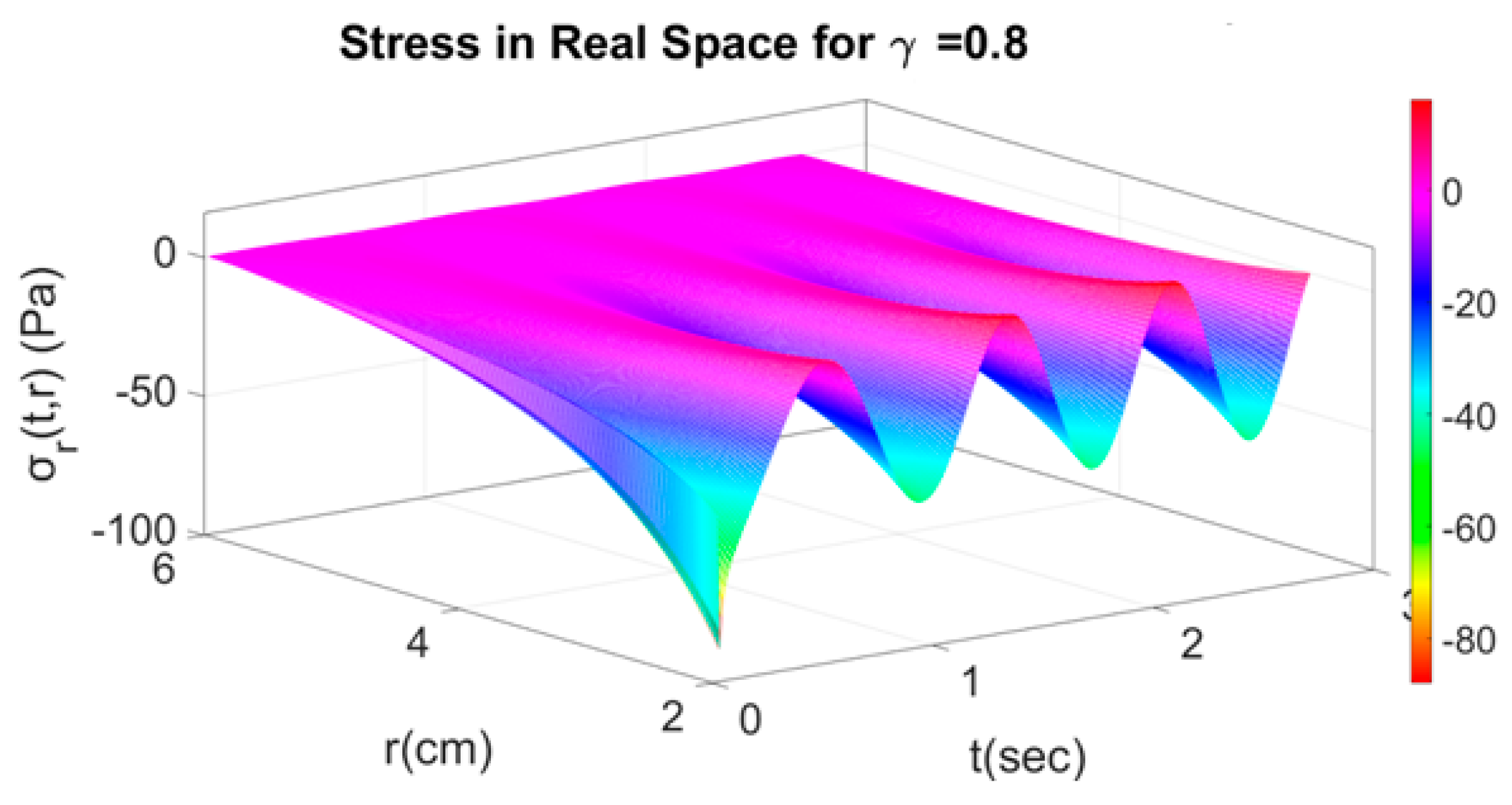
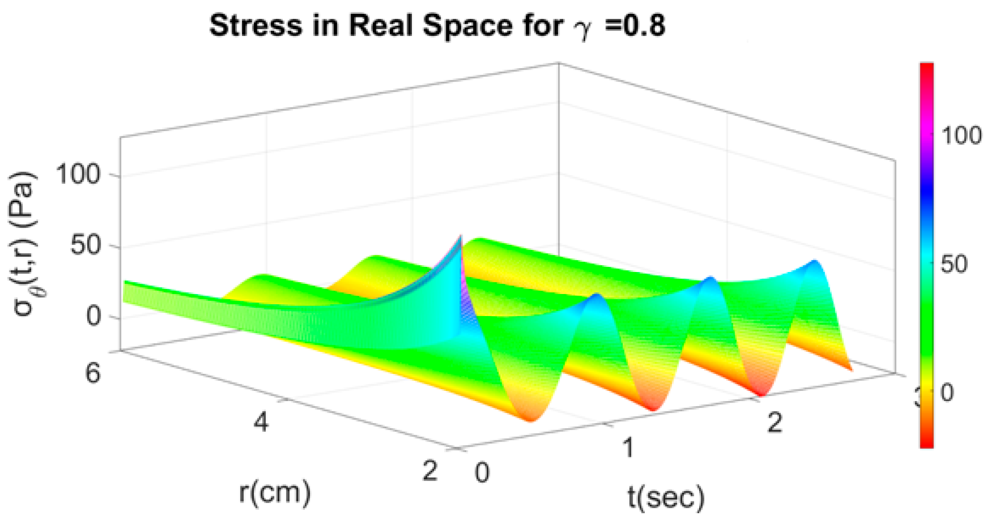
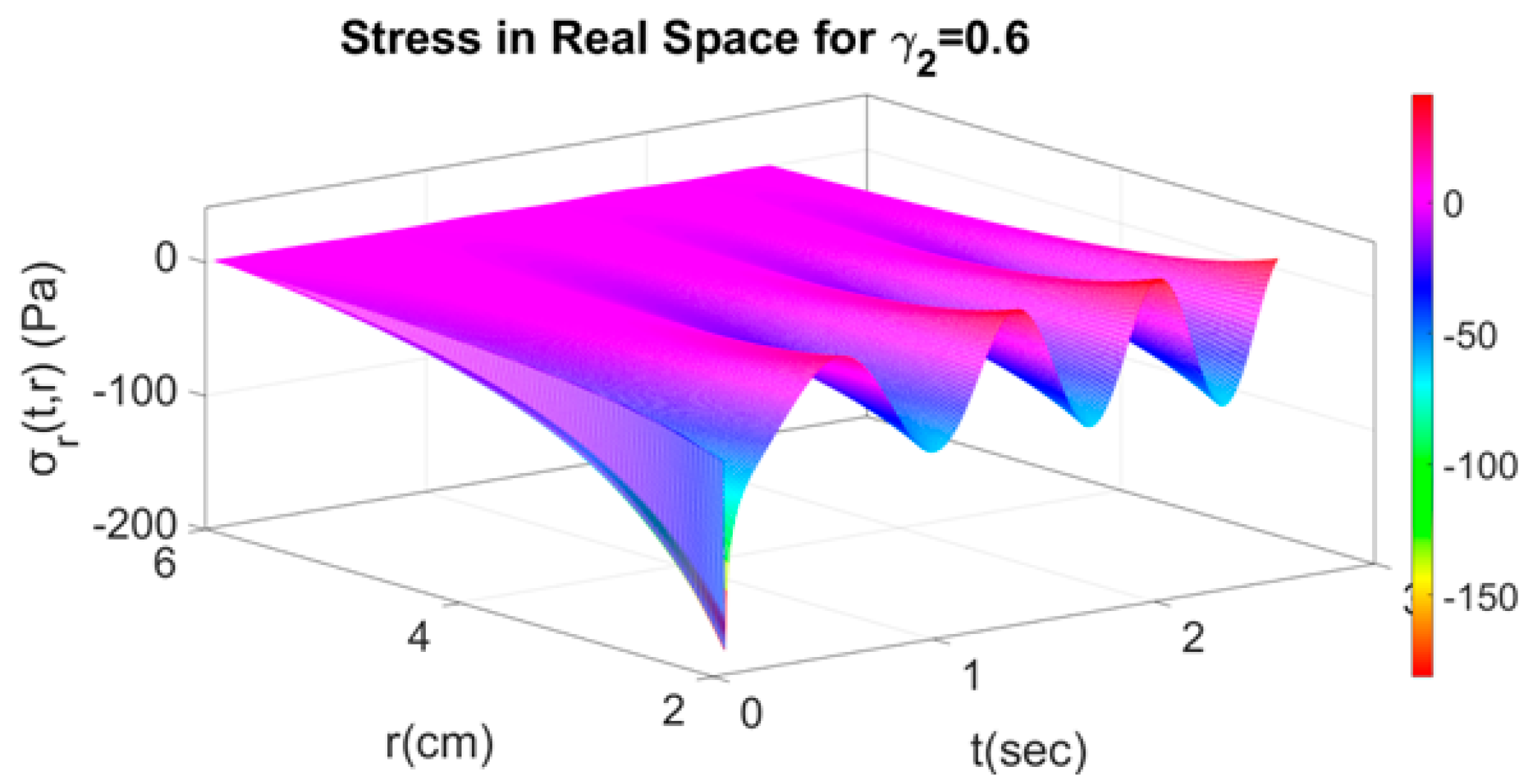
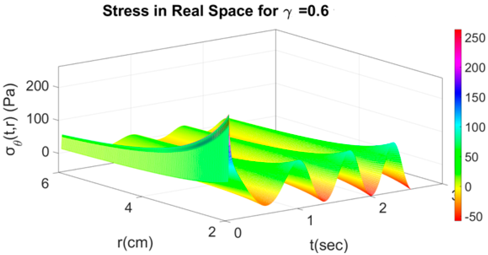
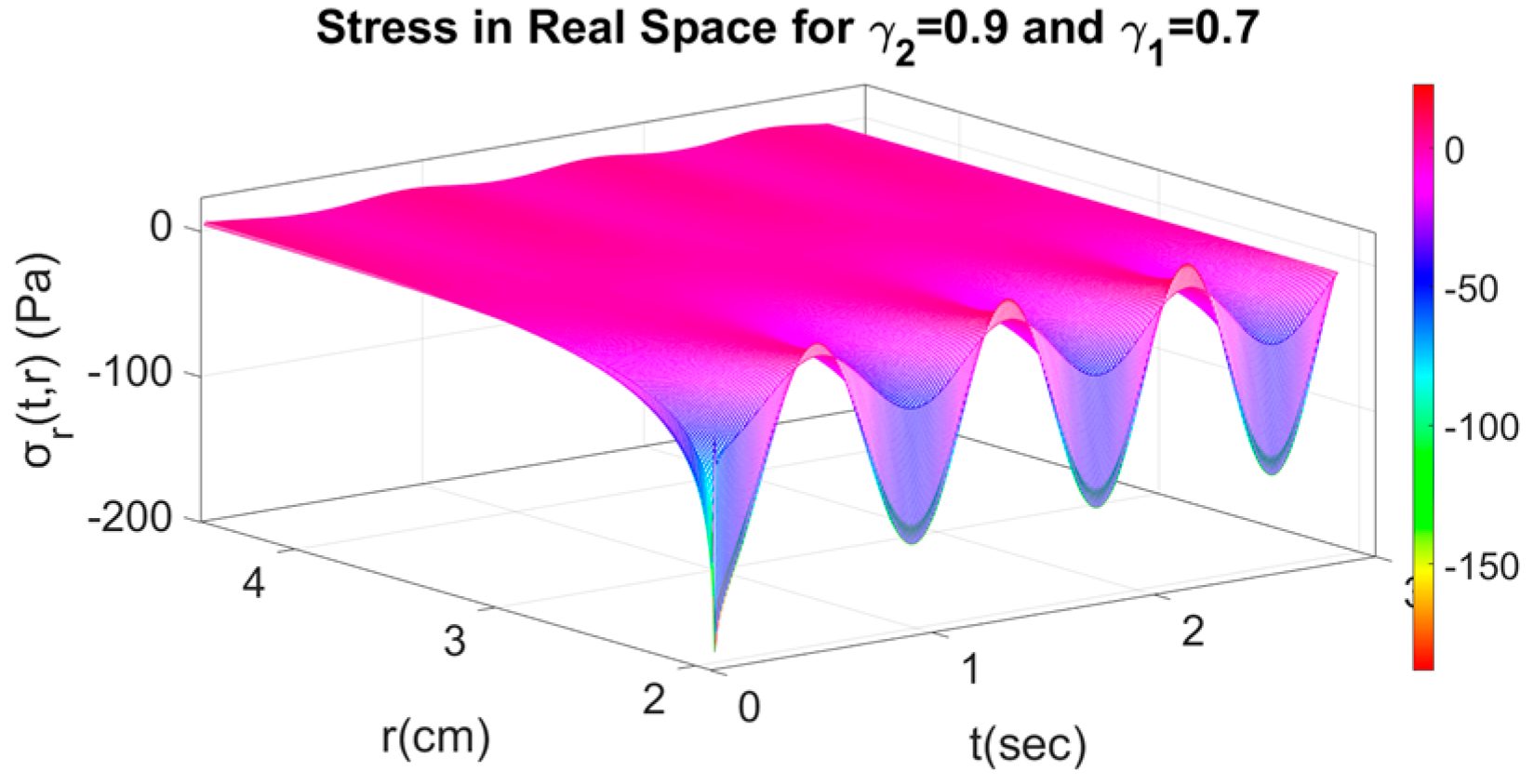
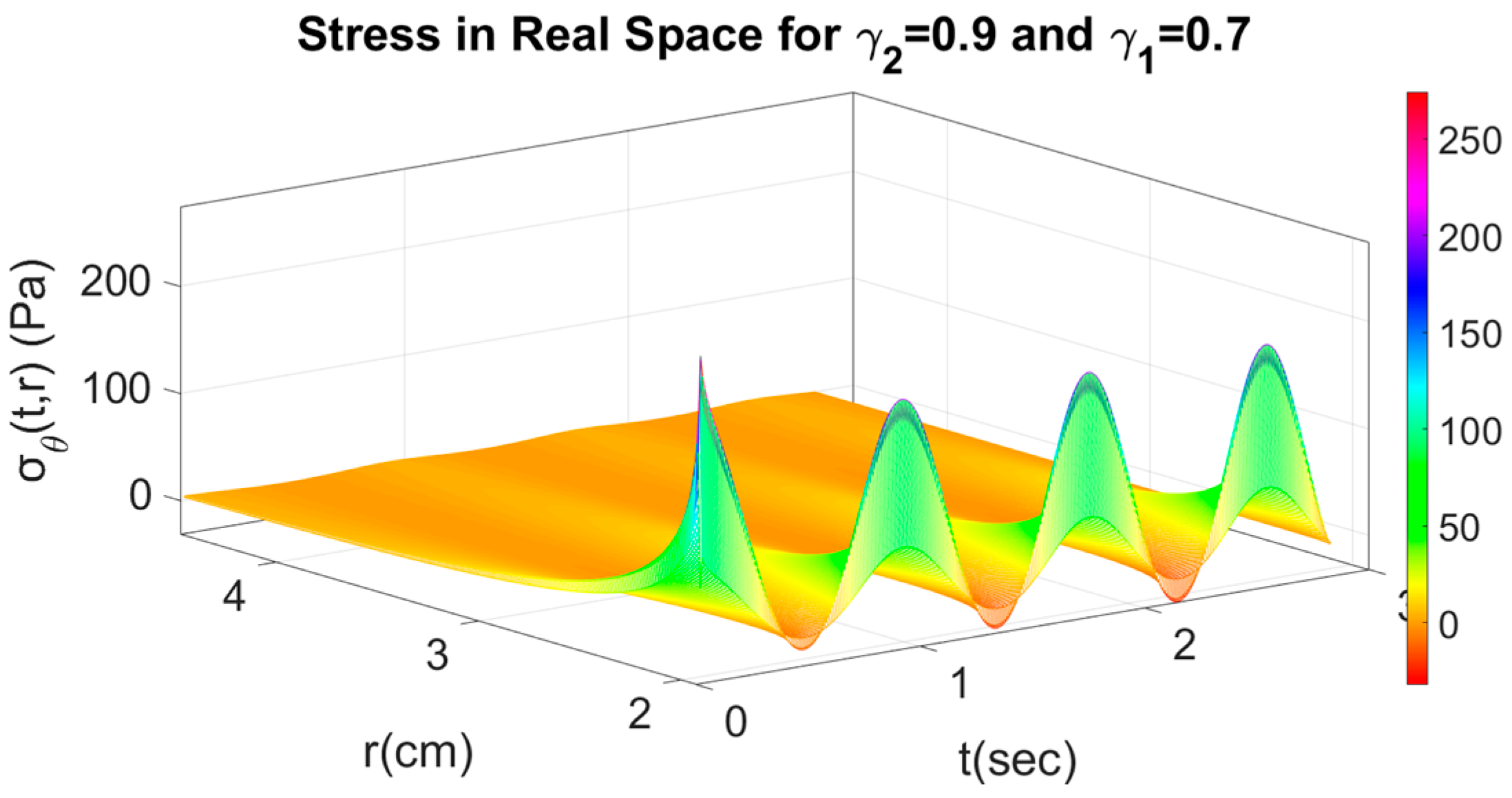
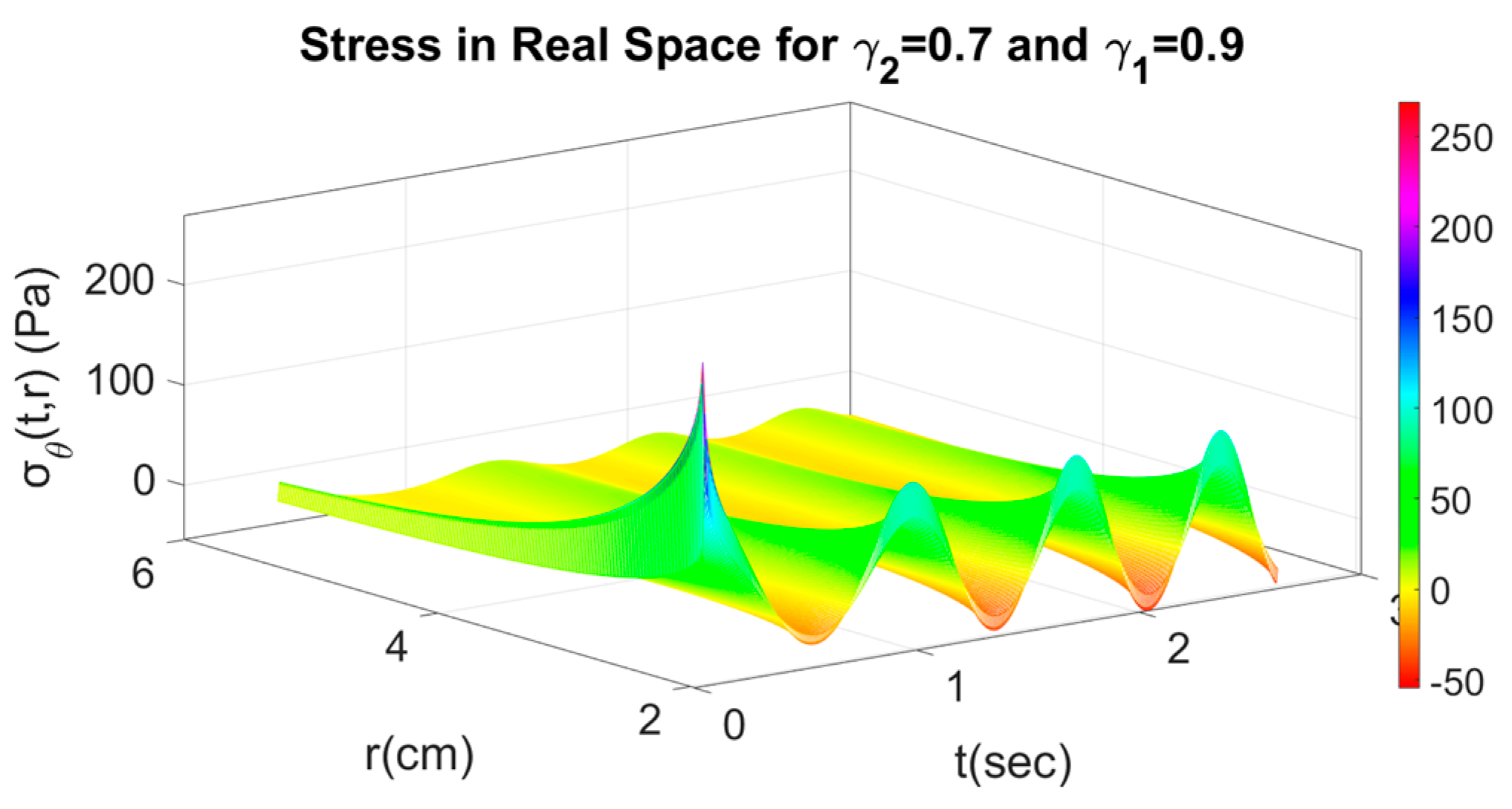
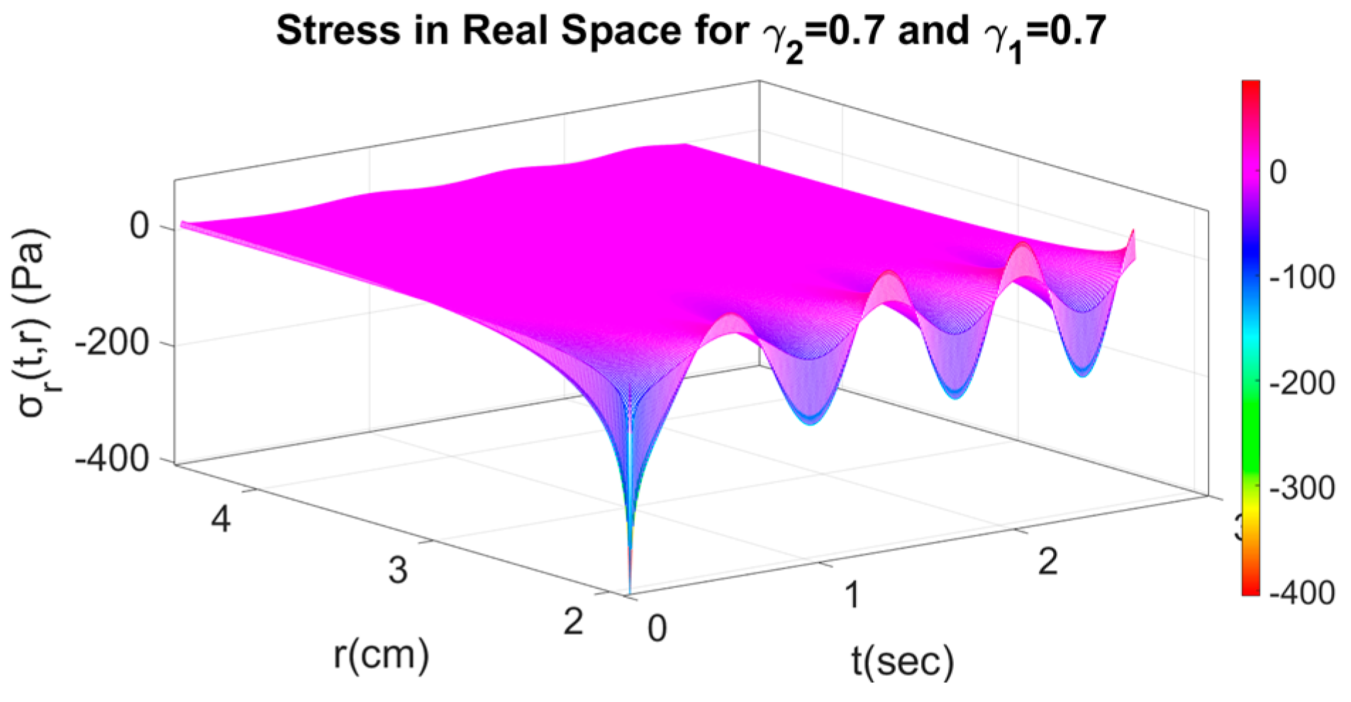
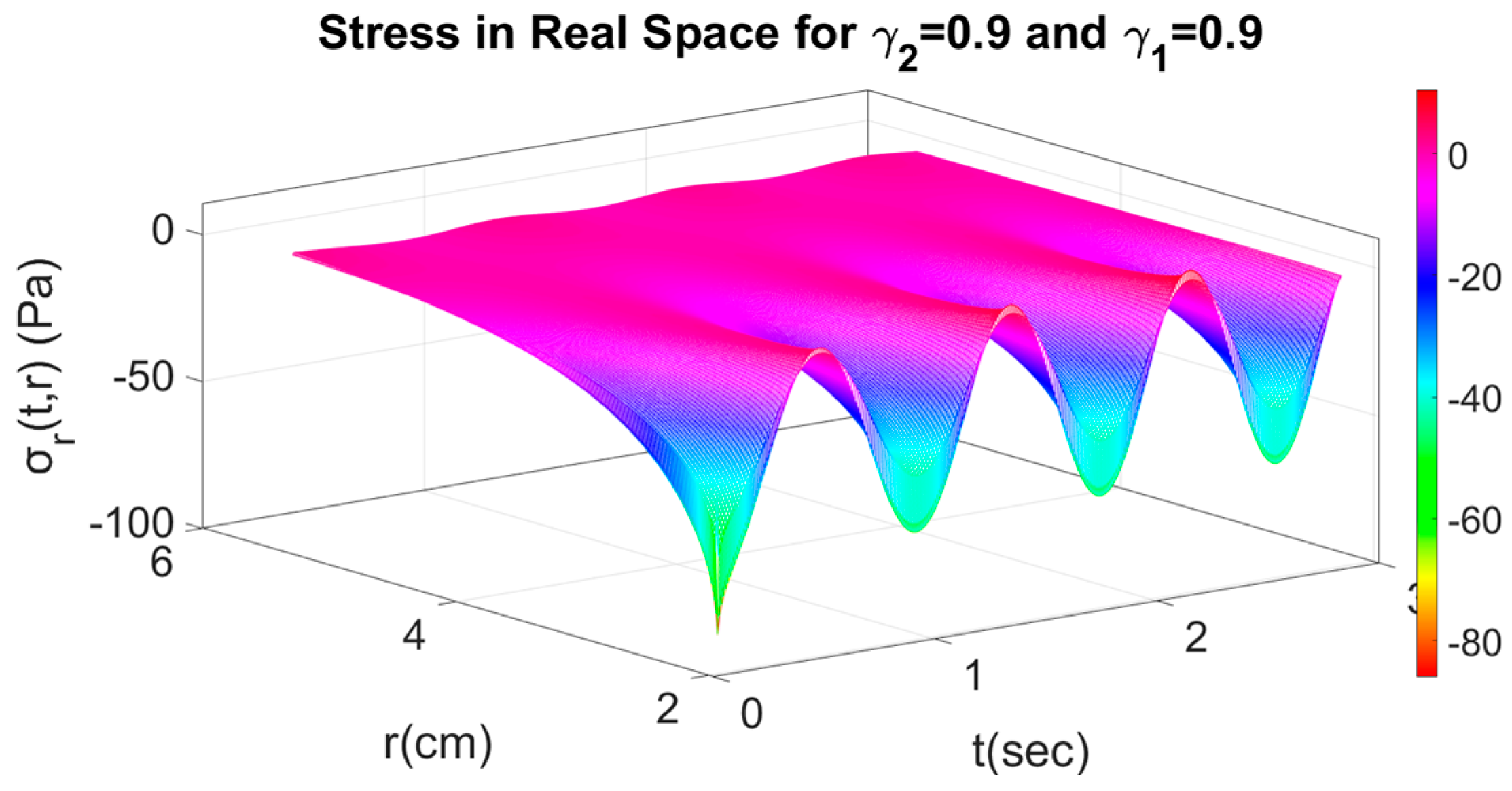
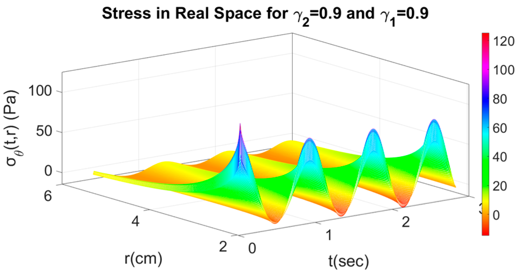
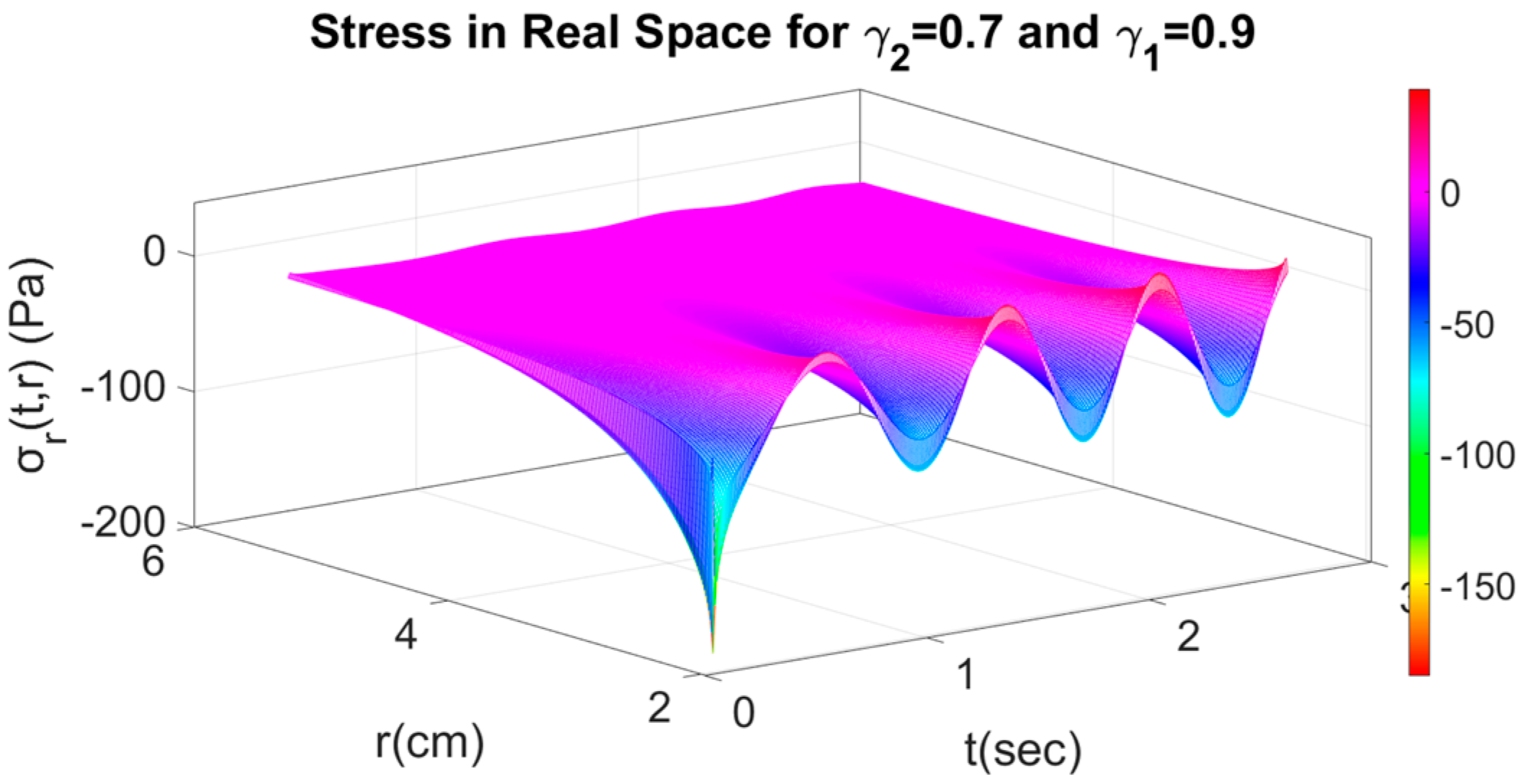
4.2. Fractional Response with Respect to Time and Space

As it has been pointed out, the fractional response with respect to time corresponds to the viscoelastic reaction of the material, whereas the fractional response with respect to the special variable R corresponds to the porosity of the material. In that case, space variable transferring should be adopted apart from the time variable transferring. Hence, if γ₂ denotes the fractional order of time and γ₁ the fractional space order of the radius r, corresponding to the radius R in the Λ-fractional space, the transformation from the Λ-fractional space (T,R) to the initial space (t,r) is defined through the relations

$$R=\frac{1}{\Gamma \left(1-{\gamma }_1\right)}{{\displaystyle \int }}_0^r\frac{q}{{\left(r-q\right)}^{{\gamma }_1}}=\frac{t^{2-{\gamma }_1}}{\Gamma \left(3-{\gamma }_1\right)},$$

(36)

$$r={\left(\Gamma \left(3-{\gamma }_1\right)R\right)}^{\frac{1}{2-{\gamma }_1}},$$

(37)

and,

$$T=\frac{1}{\Gamma \left(1-{\gamma }_2\right)}{{\displaystyle \int }}_0^t\frac{\tau }{{\left(t-\tau \right)}^{{\gamma }_2}}=\frac{r^{2-{\gamma }_2}}{\Gamma \left(3-{\gamma }_2\right)},$$

(38)

$$t={\left(\Gamma \left(3-{\gamma }_2\right)T\right)}^{\frac{1}{2-{\gamma }_2}}.$$

(39)

Hence,

$$\sigma \left(t,r\right)={}_0{}^{RL}D{}_t^{1-{\gamma }_2}\left({}_{r_1}{}^{RL}D{}_r^{1-{\gamma }_1}\left(\Sigma \left(\tau ,q\right)\right)\right)=\frac{1}{\Gamma \left({\gamma }_2\right)\cdot \Gamma \left({\gamma }_1\right)}\cdot \frac{d}{dt}{{\displaystyle \int }}_0^t\frac{1}{{(t-\tau )}^{1-{\gamma }_2}}(\frac{d}{ds}{{\displaystyle \int }}_0^r\frac{\Sigma \left(\tau ,q\right)}{{(s-q)}^{1-{\gamma }_1}}dq)d\tau .$$

(40)

Applying Equation (40) for transferring the stresses Σ_r(T,R) and Σ_θ(T,R) from the Λ-fractional space to the initial one, the radial stress σ_r(t,r) and the stress σ_θ(t,r) are defined. Indeed, Figure 12 and Figure 13 show the stresses for space fractional order γ₁ = 0.9, indicating the porosity of the material and the time fractional order γ₂ = 0.9.

Decreasing the space (porosity) order to γ₁ = 0.7, while the time (viscosity) fractional order remains the same, γ₂ = 0.9, the stress distribution for the radial σ_r(t,r) and the stress σ_θ(t,r) is shown in Figure 14 and Figure 15.

For the space (porosity) order to γ₁ = 0.9, while decreasing the time (viscosity) fractional order γ₂ = 0.7, the stress distribution for the radial σ_r(t,r) and the stress σ_θ(t,r) is shown in Figure 16 and Figure 17.

Figure 12, Figure 13, Figure 14, Figure 15, Figure 16, Figure 17, Figure 18 and Figure 19 show the influence of the fractional orders, time and space, upon the stresses. The less the fractional time–fractional order or the space (porosity) fractional order, the higher the stresses.

5. Conclusions

In this study, a Λ-fractional viscoelastic and poroelastic model was presented describing the brain of an infant exhibiting hydrocephalus phenomena. We determined that fractional calculus is a suitable analysis for studying biomechanics since fractional calculus is a non-local analysis suitable for dealing with micromechanics. However, the well-known fractional derivatives cannot generate differential geometry, and their use in solving real-life problems is questionable. Therefore, Λ-fractional analysis was applied in the present hydrocephalus model and generated differential geometry used in the model study. Continuum micromechanics was recalled to describe the present problem concerning the deformation of the hydrocephalus tube under fluid pressure. Apart from viscoelasticity, the proposed Λ-fractional model considers the influence of the tube’s porosity and the viscous material’s interaction with porous geometry. Recent references concerning hydrocephalus, mainly medical novelties, may be found in ref. [13]. The present Λ-fractional analysis may be considered a prototyped model for other cases in biomechanics.

References

1. Wilkie, K.P.; Drapaca, C.S.; Sivaloganathan, S. A nonlinear viscoelastic fractional derivative model of infant hydrocephalus. Appl. Math. Comput. 2011, 217, 8693–8704. [Google Scholar] [CrossRef]
2. Chillingworth, D.R.J. Differential Topology with a View to Applications; Pitman: London, UK; San Francisco, CA, USA, 1976. [Google Scholar]
3. Lazopoulos, K.A.; Lazopoulos, A.K. On Λ-fractional Elastic Solid Mechanics. Meccanica 2022, 57, 775–791. [Google Scholar] [CrossRef]
4. Lazopoulos, K.A.; Lazopoulos, A.K. On plane Λ-fractional linear elasticity theory. Theor. Appl. Mech. Lett. 2020, 10, 270–275. [Google Scholar] [CrossRef]
5. Drapaca, C. Brain Biomechanics: Dynamical Morphology and Nonlinear Viscoelastic Models of Hydrocephalus. Ph.D. Thesis, University of Waterloo, Waterloo, ON, Canada, 2002. [Google Scholar]
6. Drapaca, C.S.; Sivaloganathan, S. Mathematical Modelling and Biomechanics of Brain; Fields Institute, Monographs; Springer: New York, NY, USA, 2019; Volume 37. [Google Scholar]
7. Hakim, S.; Venegas, J.; Burton, J. The physics of the cranial cavity, hydrocephalus and normal pressure hydrocephalus: Mechanical interpretation and mathematical model. Surg. Neurol. 1976, 5, 187–210. [Google Scholar] [PubMed]
8. Atanackovic, T.; Philipovic, S.; Stankovic, B.; Zorica, D. Fractional Calculus with Applications in Mechanics, Vibrations and Diffusion Processes; Wiley: New York, NY, USA, 2014. [Google Scholar]
9. Drapaca, C.S.; Sivaloganathan, S.; Tenti, G.; Brake, J. Dynamical morphology of the brain’s ventricular cavities in hydrocephalus. J. Theor. Med. 2005, 6, 151–160. [Google Scholar] [CrossRef] [Green Version]
10. Samko, S.G.; Kilbas, A.A.; Marichev, O.I. Fractional Integrals and Derivatives: Theory and Applications; Gordon and Breach: Amsterdam, The Netherlands, 1993. [Google Scholar]
11. Podlubny, I. Fractional Differential Equations; An Introduction to Fractional Derivatives, Fractional Differential Equations, Some Methods of Their Solution and Some of Their Applications; Academic Press: San Diego, CA, USA, 1999. [Google Scholar]
12. Oldham, K.B.; Spanier, J. The Fractional Calculus; Academic Press: New York, NY, USA; London, UK, 1974. [Google Scholar]
13. McAlister, P., II; Talcott, M.R.; Isaacs, A.M.; Zwick, S.H.; Garcia-Bonilla, M.; Castaneyra-Ruiz, L.; Hartman, A.L.; Dilger, R.N.; Fleming, S.A.; Golden, R.K.; et al. A novel model of acquired hydrocephalus for evaluation of neurosurgical treatments. Fluids Barriers CNS 2021, 18, 49. [Google Scholar] [CrossRef] [PubMed]
Figure 1. The hydrocephalus model.
Axioms 11 00638 g001
Figure 2. The ventricular cylinder’s radial stress Σ-(T,R).
Axioms 11 00638 g002
Figure 3. The stress Σθ(T,R) in the Λ-fractional space.
Axioms 11 00638 g003
Figure 4. Distribution of the radial stress σ r ( t , r ) in the initial space for γ = 0.9.
Axioms 11 00638 g004
Figure 5. Distribution of the stress σ θ ( t , r ) in the initial space for γ = 0.9.
Axioms 11 00638 g005
Figure 6. Distribution of the radial stress σ r ( t , r ) in the initial space for γ = 0.8.
Axioms 11 00638 g006
Figure 7. Distribution of the stress σ θ ( t , r ) in the initial space for γ = 0.8.
Axioms 11 00638 g007
Figure 8. Distribution of the radial stress σ r ( t , r ) in the initial space for γ = 0.7.
Axioms 11 00638 g008
Figure 9. Distribution of the stress σ θ ( t , r ) in the initial space for γ = 0.8.
Axioms 11 00638 g009
Figure 10. Distribution of the radial stress σ r ( t , r ) in the initial space for γ = 0.6.
Axioms 11 00638 g010
Figure 11. Distribution of the stress σ θ ( r , t ) in the initial space for γ = 0.6.
Axioms 11 00638 g011
Figure 12. Distribution of the radial stress σ r ( t , r ) in the initial space with space (porosity) fractional order γ1 = 0.9 and time fractional order γ2 = 0.9.
Axioms 11 00638 g012
Figure 13. Distribution of the stress σ θ ( t , r ) in the initial space with space (porosity) fractional order γ1 = 0.9 and time fractional order γ2 = 0.9.
Axioms 11 00638 g013
Figure 14. Distribution of the radial stress σ r ( t , r ) in the initial space with space (porosity) fractional order γ1 = 0.7 and time fractional order γ2 = 0.9.
Axioms 11 00638 g014
Figure 15. Distribution of the stress σ θ ( t , r ) in the initial space with space (porosity) fractional order γ1 = 0.7 and time fractional order γ2 = 0.9.
Axioms 11 00638 g015
Figure 16. Distribution of the radial stress σ r ( t , r ) in the initial space with space (porosity) fractional order γ1 = 0.9 and time fractional order γ2 = 0.7.
Axioms 11 00638 g016
Figure 17. Distribution of the stress σ θ ( t , r ) in the initial space with space (porosity) fractional order γ1 = 0.9 and time fractional order γ2 = 0.7.
Axioms 11 00638 g017
Figure 18. Distribution of the radial stress σ r ( t , r ) in the initial space with space (porosity) fractional order γ1 = 0.7 and time fractional order γ2 = 0.7.
Axioms 11 00638 g018
Figure 19. Distribution of the stress σ θ ( t , r ) in the initial space with space (porosity) fractional order γ1 = 0.7 and time fractional order γ2 = 0.7.
Axioms 11 00638 g019
Publisher’s Note: MDPI stays neutral with regard to jurisdictional claims in published maps and institutional affiliations.