Article

Almost Periodic Solution for Forced Perturbed Non-Instantaneous Impulsive Model

Department of Mathematics, Guizhou University, Guiyang 550025, China
*
Author to whom correspondence should be addressed.
Axioms 2022, 11(10), 496; https://doi.org/10.3390/axioms11100496
Submission received: 11 August 2022 / Revised: 17 September 2022 / Accepted: 21 September 2022 / Published: 23 September 2022
(This article belongs to the Special Issue Impulsive, Delay and Fractional Order Systems)

Abstract

:
In this paper we investigate a forced perturbed non-instantaneous impulsive model. Firstly, we prove the existence and uniqueness of an almost periodic solution for the model considered by the Banach contraction principle. Secondly, we prove that all solutions converge exponentially to the almost periodic solution. In other words, the solution of the model considered is exponentially stable. Finally, we provide some simulations to show the effectiveness of the theoretical results.

1. Introduction

Differential equations have been used to simulate many phenomena in the fields of life sciences, biology, physics and engineering sciences, such as population dynamics, epidemiology, pharmacokinetics and geophysical fluid flows [1,2,3,4].
However, these systems are often seriously disturbed by short-term fluctuations in the environment. To obtain a more accurate description of such systems, we need to consider impulsive differential equations. In recent years, impulsive differential equations have been intensively investigated [5,6,7]. The investigation of these problems has important guiding significance for the exploitation and control of biological resources.
To describe some biological systems that are subjected to forced perturbation, Stamova and Stamov [8] proposed a forced perturbed model with impulsive effects at fixed moments as follows:
w ( ι ) = A ( ι ) w ( ι ) + g ( ι ) + μ W ( ι , w ( ι ) , μ ) , ι ι i , Δ w ( ι i ) = B i w ( ι i ) + g i + μ W i ( w ( ι i ) , μ ) , i N + ,
where ι 0 , ι i ( 0 ι 1 < ι 2 < ) denotes the time, which comprises impulses; w denotes the first differential of the dependent variable; w P C ( [ 0 , ; R + n ) ; A C ( [ 0 , ) , R n × n ) ; Δ w ( ι i ) = w ( ι i + ) w ( ι i ) ; w ( ι i + ) denotes the right limits of w ( ι i ) and w ( ι i ) denotes the left limits of w ( ι i ) ; P C ( [ 0 , ) R n ) : = { w : [ 0 , ) R n : w C ( ( m i , m i + 1 ] , R n ) ; w ( m i ) and w ( m i + ) exist; w ( m i ) = w ( m i ) ; i N + } , g C ( [ 0 , ) R n ) , C ( [ 0 , ] , R n ) represents the space that is made up of all continuous functions from [ 0 , ] to R n ; μ M R ; W : [ 0 , ) × R + n × M R n ; B i R n × n ; g i R n ; W i : R + n × M R n , i N + ; x = ( x 1 , x 2 , , x n ) , N : = { 0 , 1 , 2 , 3 , } and N + : = N / { 0 } .
Then, Stamova and Stamov demonstrated the existence and uniqueness of an almost periodic solution (AP) of model (1) and the exponential stability of the solution.
However, most systems do not return to normal immediately after the impulses and stay active for a limited period of time. Therefore, Hernández et al. [9] firstly introduced the theory of non-instantaneous impulses and established the existence of solutions for a class of impulsive differential equations. After that, Wang et al. [10,11,12] generalized the non-instantaneous impulsive model and carried out more in-depth research on non-instantaneous impulsive differential equations. In general, there are no impulses that occur instantaneously, that is to say, they are non-instantaneous, even if the event occurs over a short period of time. Therefore, it is essential to consider a class of differential equations with non-instantaneous impulses.
According to the actual condition, we consider the following model (2), which is model (1) including non-instantaneous impulses:
w ( ι ) = A ( ι ) w ( ι ) + g ( ι ) + μ W ( ι , w , μ ) , ι ( l i , m i + 1 ] , i N , w ( m i + ) = B i w ( m i ) + g i + μ W i ( w ( m i ) , μ ) , i N + , w ( ι ) = B i w ( m i ) + g i + μ W i ( w ( m i ) , μ ) , ι ( m i , l i ] , i N + , w ( l i + ) = w ( l i ) , i N + ,
where 0 = l 0 < m 1 < l 1 < m 2 < l 2 < < m i < l i < m i + 1 < .
Let w ( ι , μ ) = w ( ι ; ι 0 , w 0 , μ ) be the solution of model (2) with the initial condition w ( ι 0 + , μ ) = w 0 , w 0 R + n , μ M .
Periodic phenomena are widespread natural phenomena [13], but most of the changes are not integer time periods. Therefore, we should consider parameters that are AP in the natural environment. Many scholars have demonstrated that it is more realistic to adopt an AP hypothesis in the process of AP study, when taking into account the impact of environmental factors, and this has certain ergodicity [14,15,16,17,18]. Therefore, a series of studies on AP solutions of model (2) are carried out in this paper.
The rest of this paper is arranged as follows. In Section 2, we provide some of the necessary preliminaries. In Section 3, we prove the existence and uniqueness of the AP solution to model (2). In Section 4, we investigate that the solution of model (2) is exponentially stable. In Section 5, some simulations are given to support our theoretical results.

2. Preliminaries

For the sequences { m i } and { l i } , i N + , assume lim i + m i = + , lim i + l i = + and l i 1 < m i < l i < m i + 1 , let j = i = 1 n j i 2 1 2 for j = ( j 1 , j 2 , , j n ) . Let λ max ( · ) be the largest eigenvalue of ( · ) and X = λ max ( X X ) for the matrix X. The space P C ( [ 0 , ) , R n ) equipped with the norm w P C = sup ι [ 0 , ) w ( ι ) . It is obvious that ( P C ( [ 0 , ) , R n ) , · P C ) is a Banach space.
Set
B h ( a ) = { x R n , x a < h } , h > 0 , a R n .
Definition 1
(see [19]). For the sequences { M i } i N + , M i R n , if for any i N + there exists ε > 0 and integer p such that the following inequality holds
M i + p M i < ε ,
then p is called the ε-AP of the { M i } i N + , M i R n .
Definition 2
(see [20]). { M i } i N + , M i R n are called AP sequences if for any ε > 0 there exists a relatively dense set of its ε-AP.
Definition 3
(see [19]). The w P C ( [ 0 , ) , R n ) is called an AP function if all of the conditions are met as follows
(i) { m i j } , i , j N + are uniform AP sequences, where m i j = m i + j m i .
(ii) For any ε > 0 , there exists a number δ = δ ( ε ) , which is positive such that if ι 1 and ι 2 are the points in the same continuous interval and | ι 1 ι 2 | < δ , then w ( ι 1 ) w ( ι 2 ) < ε .
(iii) For any ε > 0 , there exists a relatively dense set Γ of ε -AP such that if ϑ Γ , then w ( ι + ϑ ) w ( ι ) < ε for all ι [ 0 , ) satisfying the condition | ι m i | > ε , i N + .
In order to study the AP property of model (2), we propose some assumptions as follows.
( H 1 ) The sequences { l i j } , l i j = l i + j l i and { m i j } , m i j = m i + j m i , i , j N + are uniformly AP and 0 < l i m i θ < + , 0 < ς m i + 1 l i θ ¯ < + , i N + .
( H 2 ) The matrix function A C ( [ 0 , ) , R n × n ) is AP in the sense of Bohr.
( H 3 ) The sequence { B i } , i N + is an AP sequence.
( H 4 ) The function g C ( [ 0 , ) , R n ) is AP.
( H 5 ) { g i } , i N + is an AP sequence.
( H 6 ) The function W C ( [ 0 , ) × R + n × M , R n ) is AP in ι uniformly with respect to ( w , μ ) R + n × M and Lipschitz continuous with respect to w B h with a Lipschitz constant L 1 > 0 such that
W ( ι , w , μ ) W ( ι , w ˜ , μ ) L 1 w w ˜ , w , w ˜ B h ,
for any ι [ 0 , ) and μ M .
( H 7 ) The sequence of functions { W i ( w , μ ) } , i N + , W i C ( R + n × M , R n ) is AP uniform with respect to ( w , μ ) R + n × M and the functions W i are Lipschitz-continuous with respect to w B h with a Lipschitz constant L 2 > 0 such that
W i ( w , μ ) W i ( w ˜ , μ ) L 2 w w ˜ , w , w ˜ B h ,
for i N + , μ M .
Lemma 1
(see [19]). Let conditions ( H 1 ) ( H 5 ) hold. Then, for each ε > 0 , there exists ε 1 , 0 < ε 1 < ε , a relatively dense set Γ of real numbers and a set Q of integers such that the following relations are fulfilled.
(a) A ( ι + ϑ ) A ( ι ) < ε , ι [ 0 , ) , ϑ Γ ;
(b) g ( ι + ϑ ) g ( ι ) < ε , ι [ 0 , ) , | ι m i | > ε , | ι l i | > ε , i N + ;
(c) B i + q B i < ε , g i + q g i < ε , q Q , i N + ;
(d) | l i q ϑ | < ε 1 , | m i q ϑ | < ε 1 , q Q , ϑ Γ , i N + .
Lemma 2
(see [8]). Assume that conditions ( H 1 ) , ( H 4 ) and ( H 5 ) hold, then there exists a positive constant C such that
max sup ι [ 0 , ) g ( ι ) , sup i N + g i C .
Denote the number of impulse points m i in the interval ( s , ι ) as k ( ι , s ) .
Lemma 3
(see [19]). If the sequences { m i j } , i , j N are uniformly AP, then we can obtain
( i ) There exists a constant ρ > 0 such that sup t + k ( ι + t , ι ) t = ρ , which is uniform with respect to ι > 0 .
( i i ) For any p > 0 , there exists N, which is a positive integer such that the number of elements in the sequence { m i } on each interval of length p does not exceed N. We can choose N ρ .
Definition 4.
The model
w ( ι ) = A ( ι ) w ( ι ) + g ( ι ) , ι ( l i , m i + 1 ] , i N , w ( m i + ) = B i w ( m i ) + g i , i N + , w ( ι ) = B i w ( m i ) + g i , ι ( m i , l i ] , i N + , w ( l i + ) = w ( l i ) , i N + ,
is said to be a generating model of model (2).
Consider
w ( ι ) = A ( ι ) w ( ι ) , ι ( l i , m i + 1 ] , i N , w ( m i + ) = B i w ( m i ) , i N + , w ( ι ) = B i w ( m i ) , ι ( m i , l i ] , i N + , w ( l i + ) = w ( l i ) , i N + .
Let w ( ι ) = W ( ι , ι 0 ) w ι 0 , 0 ι 0 ι represent the solution of model (5) with w ( ι 0 ) = w ι 0 , where W ( ι , ι 0 ) is the Cauchy matrix of model (5), which can be looked up in [21].
Lemma 4
(see [21]). Assume that ( H 1 ) ( H 3 ) hold, the Cauchy matrix W ( ι , ι 0 ) of model (5) is exponentially stable and W ( ι , ι 0 ) Ξ e Y ( ι ι 0 ) , Ξ 1 , Y > 0 .
Lemma 5
(see [21]). For any ε > 0 , 0 ι 0 < ι , | ι m i | > ε , | ι l i | > ε , | ι 0 m i | > ε and | ι 0 l i | > ε , i N + , there exists a constant K > 0 and a relatively dense set of Γ of ε-AP such that
W ( ι + ϑ , ι 0 + ϑ ) W ( ι , ι 0 ) ε K e 1 2 Y ( ι ι 0 ) , ϑ Γ .

3. Existence and Uniqueness of Almost Periodic Solution

In this section, we study the existence and uniqueness of a positive AP solution for model (2).
We propose the condition as follows.
( H 8 ) There exists a positive constant L such that
max sup ι [ 0 , ) ( w , μ ) R + n × M W ( ι , w , μ ) , sup i N + ( w , μ ) R + n × M W i ( w , μ ) L .
Theorem 1.
Assume that ( H 1 ) ( H 8 ) hold, model (2) has a unique positive AP solution if
| μ | Ξ L 1 Y + N 1 L 2 < 1 ,
where Ξ and Y are given in Lemma 4.
Proof. 
Let N 1 = sup ι [ 0 , ) i = 1 k ( ι , 0 ) e Y ( ι m i + ) < + , N 2 = sup ι [ 0 , ) i = 1 k ( ι , 0 ) e Y 2 ( ι m i + ) < + and Ω : = { w : w P C ( [ 0 , ) , R + n ) , w is AP ( w ( · + ϑ ) w ( · ) P C < ε , ϑ Γ ) and w P C C } , where Γ is mentioned in Lemma 1, C = Ξ ( C + | μ | L ) 1 Y + N 1 .
For l i < ι < m i + 1 , i N , we define the operator T,
( T w ) ( ι ) = i = 0 k ( ι , 0 ) 1 l i m i + 1 W ( ι , τ ) ( g ( τ ) + μ W ( τ , w ( τ , μ ) , μ ) ) d τ + l k ( ι , 0 ) ι W ( ι , τ ) ( g ( τ ) + μ W ( τ , w ( τ , μ ) , μ ) ) d τ + i = 1 k ( ι , 0 ) W ( ι , m i + ) ( g i + μ W i ( w ( m i + , μ ) , μ ) ) .
From Lemmas 2 and 4, for any w Ω it follows that
( T w ) ( ι ) i = 0 k ( ι , 0 ) 1 l i m i + 1 W ( ι , τ ) ( g ( τ ) + | μ | W ( τ , w ( τ , μ ) , μ ) ) d τ + l k ( ι , 0 ) ι W ( ι , τ ) ( g ( τ ) + | μ | W ( τ , w ( τ , μ ) , μ ) ) d τ + i = 0 k ( ι , 0 ) W ( ι , m i + ) ( g i + | μ | W i ( w ( m i + , μ ) , μ ) ) 0 ι Ξ e Y ( ι τ ) ( C + | μ | L ) d τ + Ξ i = 1 k ( ι , 0 ) e Y ( ι m i + ) ( C + | μ | L ) Ξ ( C + | μ | L ) 1 Y + N 1 .
Consequently, we obtain T ( Ω ) Ω .
Next, let ϑ Γ , q Q , | ι m i | > ε , | ι l i | > ε , we have
T w ( ι + ϑ , μ ) T w ( ι , μ ) Λ 1 + Λ 2 + Λ 3 ,
where
Λ 1 = i = 0 k ( ι , 0 ) 1 l i m i + 1 W ( ι + ϑ , τ + ϑ ) W ( ι , τ ) ( g ( τ + ϑ ) + | μ | W ( τ + ϑ , w ( τ + ϑ , μ ) , μ ) ) d τ + l k ( ι , 0 ) ι W ( ι + ϑ , τ + ϑ ) W ( ι , τ ) ( g ( τ + ϑ ) + | μ | W ( τ + ϑ , w ( τ + ϑ , μ ) , μ ) ) d τ 0 ι ε K e 1 2 Y ( ι τ ) ( C + | μ | L ) d τ 2 ε K Y ( C + | μ | L ) ,
Λ 2 = i = 0 k ( ι , 0 ) 1 l i m i + 1 W ( ι , τ ) ( g ( τ + ϑ ) g ( τ ) + | μ | W ( τ + ϑ , w ( τ + ϑ , μ ) , μ ) W ( τ , w ( τ , μ ) , μ ) ) d τ + l k ( ι , 0 ) ι W ( ι , τ ) ( g ( τ + ϑ ) g ( τ ) + | μ | W ( τ + ϑ , w ( τ + ϑ , μ ) , μ ) W ( τ , w ( τ , μ ) , μ ) ) d τ 0 ι Ξ e Y ( ι τ ) ( ε + | μ | ε ) d τ Ξ Y ( ε + | μ | ε ) ,
Λ 3 i = 0 k ( ι , 0 ) W ( ι + ϑ , m i + q + ) W ( ι , m i + ) ( g i + q + | μ | W i + q ( w ( m i + q + , μ ) , μ ) ) ) + i = 0 k ( ι , 0 ) W ( ι , m i + ) ( g i + q g i + | μ | W i + q ( w ( m i + q + , μ ) , μ ) W i ( w ( m i + , μ ) , μ ) ) ε K N 2 ( C + | μ | L ) + Ξ N 1 ( ε + | μ | ε ) .
Finally, for any w 1 , w 2 , we have
( T w 1 ) ( ι ) ( T w 2 ) ( ι ) i = 0 k ( ι , 0 ) 1 | μ | l i m i + 1 W ( ι , τ ) W ( τ , w 1 ( τ , μ ) , μ ) ) W ( τ , w 2 ( τ , μ ) , μ ) ) d τ + | μ | l k ( ι , 0 ) ι W ( ι , τ ) W ( τ , w 1 ( τ , μ ) , μ ) ) W ( τ , w 2 ( τ , μ ) , μ ) ) d τ + | μ | i = 1 k ( ι , 0 ) W ( ι , m i + ) W i ( w 1 ( m i + , μ ) , μ ) W i ( w 2 ( m i + , μ ) , μ ) | μ | 0 ι Ξ e Y ( ι τ ) L 1 w 1 w 2 P C d τ + | μ | i = 1 k ( ι , 0 ) Ξ e Y ( ι m i + ) L 2 w 1 w 2 P C | μ | Ξ L 1 1 Y w 1 w 2 P C + | μ | Ξ N 1 L 2 w 1 w 2 P C | μ | Ξ ( L 1 Y + N 1 L 2 ) w 1 w 2 P C ,
which implies that
T w 1 T w 2 P C | μ | Ξ ( L 1 Y + N 1 L 2 ) w 1 w 2 P C .
We can obtain that there exists a unique positive AP solution of model (2) when Equation (6) holds by the Banach contraction principle. □

4. Exponential Stability

Theorem 2.
Assume that in the generating model (4) there exists a unique AP solution. For | μ | 0 , w ( ι , μ ) converges to the unique AP solution of model (4).
Proof. 
Let us denote by w ( ι ) the AP solution of model (4). From Equation (7) and Definition 4, it follows that
w ( ι , μ ) w ( ι ) | μ | ( 0 ι W ( ι , τ ) W ( τ , w ( τ , μ ) , μ ) d τ + i = 1 k ( ι , 0 ) W ( ι , m i + ) W i ( w ( m i + , μ ) , μ ) ) | μ | 0 ι Ξ e Y ( ι τ ) L d τ + Ξ N 1 L | μ | Ξ L Y + Ξ N 1 L .
Then, w ( ι , μ ) w ( ι ) for | μ | 0 . □
Theorem 3.
Assume that all conditions in Theorem 1 and N ln ( 1 + | μ | Ξ L 2 ) + | μ | Ξ L 1 < Y hold. The solution w ( ι , μ ) is exponentially stable.
Proof. 
Let w ( ι ) be an arbitrary solution of model (4). Then, using Equation (7), we obtain
w ( ι ) w ( ι , μ ) = W ( ι , ι 0 ) ( w ( ι 0 ) w ( ι 0 , μ ) ) + μ ( i = k ( ι 0 , 0 ) k ( ι , ι 0 ) 1 l i m i + 1 W ( ι , τ ) ( W ( τ , w ( τ ) ) W ( τ , w ( τ , μ ) , μ ) ) d τ + l k ( ι , ι 0 ) ι W ( ι , τ ) ( W ( τ , w ( τ ) ) W ( τ , w ( τ , μ ) , μ ) ) d τ + i = k ( ι 0 , 0 ) + 1 k ( ι , ι 0 ) W ( ι , m i + ) ( W i ( w ( m i + ) ) W i ( w ( m i + , μ ) , μ ) ) ) .
Now, we obtain
w ( ι ) w ( ι , μ ) Ξ e Y ( ι ι 0 ) w ( ι 0 ) w ( ι 0 , μ ) + | μ | ( ι 0 ι Ξ e Y ( ι τ ) L 1 w ( τ ) w ( τ , μ ) d τ + i = k ( ι 0 , 0 ) + 1 k ( ι , ι 0 ) Ξ e Y ( ι m i + ) L 2 w ( m i + ) w ( m i + , μ ) ) .
Set v ( ι ) = w ( ι ) w ( ι , μ ) e Y ι , then by means of Gronwall–Bellman’s inequality [22], it follows that
w ( ι ) w ( ι , μ ) Ξ w ( ι 0 ) w ( ι 0 , μ ) e Y ( ι ι 0 ) i = k ( ι 0 , 0 ) + 1 k ( ι , ι 0 ) 1 + | μ | Ξ L 2 e Y ( ι m i + ) e ι 0 ι | μ | Ξ L 1 e Y ( ι τ ) d τ Ξ w ( ι 0 ) w ( ι 0 , μ ) e Y ( ι ι 0 ) ( 1 + | μ | Ξ L 2 ) k ( ι , ι 0 ) e | μ | Ξ L 1 ( ι ι 0 ) Ξ w ( ι 0 ) w ( ι 0 , μ ) ( 1 + | μ | Ξ L 2 ) k ( ι , ι 0 ) e ( Y + | μ | Ξ L 1 ) ( ι ι 0 ) Ξ w ( ι 0 ) w ( ι 0 , μ ) e ln ( 1 + | μ | Ξ L 2 ) k ( ι , ι 0 ) e ( Y + | μ | Ξ L 1 ) ( ι ι 0 ) Ξ w ( ι 0 ) w ( ι 0 , μ ) e ( N ln ( 1 + | μ | Ξ L 2 ) Y + | μ | Ξ L 1 ) ( ι ι 0 ) .
Obviously, if there exists N ln ( 1 + | μ | Ξ L 2 ) + | μ | Ξ L 1 < Y , then the solution of model (2) is exponentially stable. □

5. Numerical Simulations

We present two Examples and some corresponding numerical simulations in this Section. We first give the figures of solution and exponentially stable Example 1, which correspond to model (5). Then, on the basis of Example 1, we show the figures of solution and exponentially stable Example 2, which correspond to model (2).
Example 1.
Consider
w 1 ( ι ) = ( 7 + sin 2 ι ) w 1 ( ι ) + e ι 100 w 2 ( ι ) , ι ( l i , m i + 1 ] , i N , w 2 ( ι ) = e ι 100 w 1 ( ι ) + ( 7 + sin 2 ι ) w 2 ( ι ) , ι ( l i , m i + 1 ] , i N , w 1 ( m i + ) = | cos i | w 1 ( m i ) + | sin i | w 2 ( m i ) , i N + , w 2 ( m i + ) = | sin i | w 1 ( m i ) + | cos i | w 2 ( m i ) , i N + , w 1 ( ι ) = | cos i | w 1 ( m i ) + | sin i | w 2 ( m i ) , ι ( m i , l i ] , i N + , w 2 ( ι ) = | sin i | w 1 ( m i ) + | cos i | w 2 ( m i ) , ι ( m i , l i ] , i N + , w 1 ( l i + ) = w 1 ( l i ) , i N + , w 2 ( l i + ) = w 2 ( l i ) , i N + .
Assume that w ( ι ) is the solution of model (8) satisfying the initial conditions as follows
w 1 ( ι 0 + ) = 1.5 , ι 0 = 0 , w 2 ( ι 0 + ) = 2 , ι 0 = 0 .
Set l 0 = 0 , { m i } and { l i } , i N as
m i = i + 1 8 | cos i cos ( 2 i ) | , l i = i + 1 4 | cos i cos ( 2 i ) | .
By elementary calculation, we have
0 < l i m i < 1 4 , i N + , 1 2 < m i + 1 l i < 3 2 , i N , ι l k ( ι , 0 ) 0 , 3 2 .
It is obvious that m i , i N + and l i , i N are uniformly AP. Hence, model (8) satisfies conditions ( H 1 ) ( H 5 ) .
Next, according to Lemma 3, we obtain i = 0 k ( ι , 0 ) 1 ( m i + 1 l i ) > 1 2 k ( ι , 0 ) . Thus,
lim sup ι + k ( ι , 0 ) ι lim sup ι + k ( ι , 0 ) i = 0 k ( ι , 0 ) 1 ( m i + 1 l i ) < lim sup ι + k ( ι , 0 ) 1 2 k ( ι , 0 ) < 2 = N .
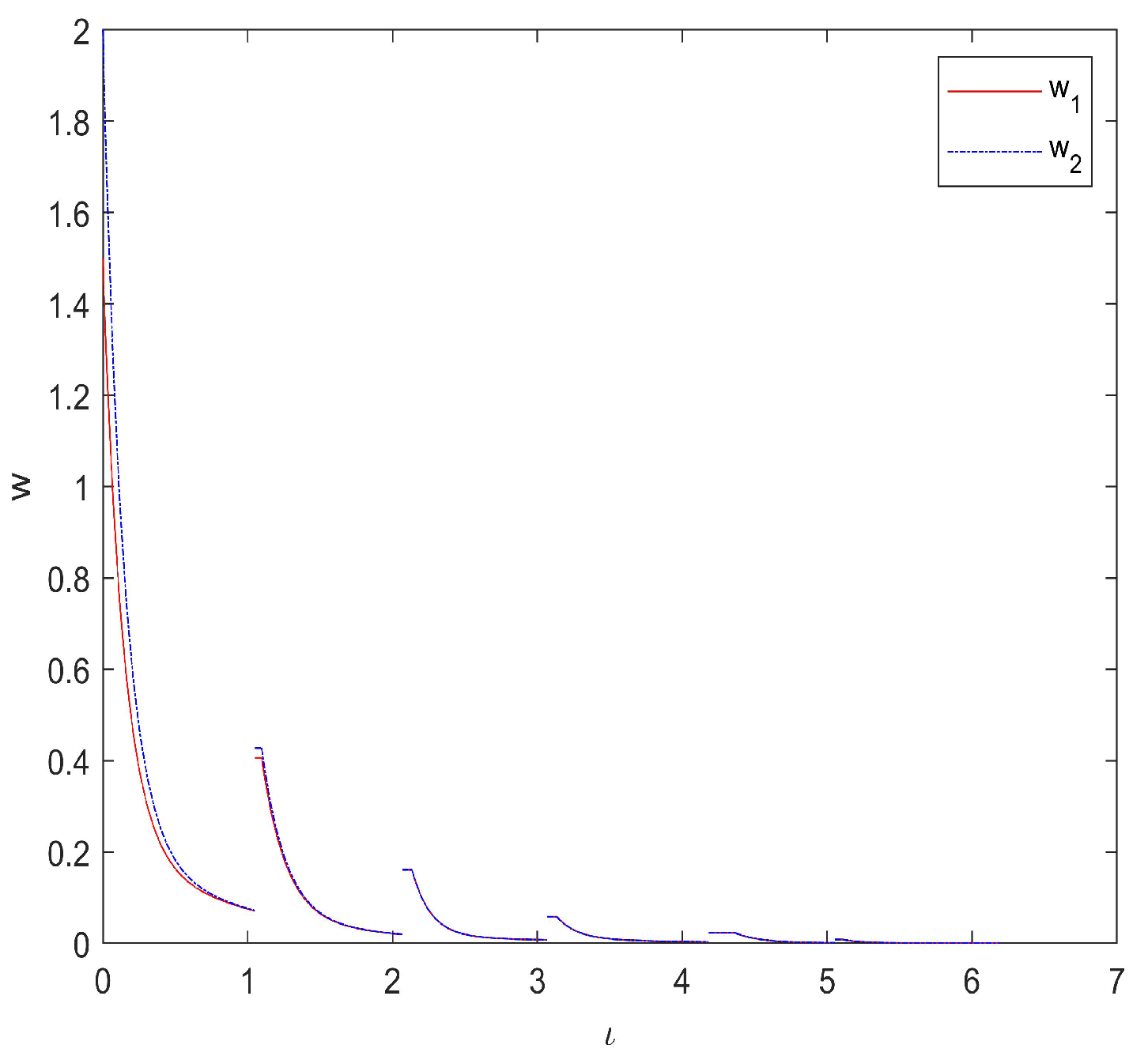
We know that model (8) with the initial condition (9) has a unique AP solution. We use Figure 1 to represent this AP solution.
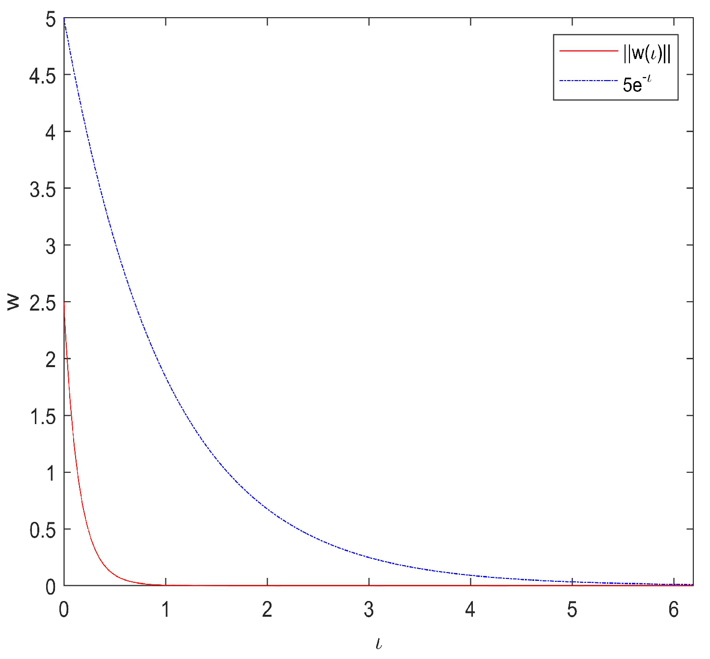
According to Lemma 4, we can conclude that model (8) is exponentially stable and has w ( ι ) 5 e ι when Ξ = 2 , Y = 1 . Then, we can represent this result in Figure 2.
Example 2.
w 1 ( ι ) = ( 7 + sin 2 ι ) w 1 ( ι ) + e ι 100 w 2 ( ι ) + e ι + 1 200 ( sin ι w 1 ( ι ) + e ι w 2 ( ι ) ) , ι ( l i , m i + 1 ] , i N , w 2 ( ι ) = e ι 100 w 1 ( ι ) + ( 7 + sin 2 ι ) w 2 ( ι ) + e ι + 1 200 ( e ι w 1 ( ι ) + sin ι w 2 ( ι ) ) , ι ( l i , m i + 1 ] , i N , w 1 ( m i + ) = | cos i | w 1 ( m i ) + | sin i | w 2 ( m i ) + e i + 1 200 ( sin i w 1 ( m i ) + 1 2 e i w 2 ( m i ) ) , i N + , w 2 ( m i + ) = | sin i | w 1 ( m i ) + | cos i | w 2 ( m i ) + e i + 1 200 ( 1 2 e i w 1 ( m i ) sin i w 2 ( m i ) ) , i N + , w 1 ( ι ) = | cos i | w 1 ( m i ) + | sin i | w 2 ( m i ) + e i + 1 200 ( sin i w 1 ( m i ) + 1 2 e i w 2 ( m i ) ) , ι ( m i , l i ] , i N + , w 2 ( ι ) = | sin i | w 1 ( m i ) + | cos i | w 2 ( m i ) + e i + 1 200 ( 1 2 e i w 1 ( m i ) sin i w 2 ( m i ) ) , ι ( m i , l i ] , i N + , w 1 ( l i + ) = w 1 ( l i ) , i N + , w 2 ( l i + ) = w 2 ( l i ) , i N + .
Assume that w ( ι , μ ) is a solution of model (10) satisfying the initial conditions as follows
w 1 ( ι 0 + , μ ) = 1.5 , ι 0 = 0 , w 2 ( ι 0 + , μ ) = 2 , ι 0 = 0 .
Set l 0 = 0 , { m i } and { l i } , i N as
m i = i + 1 8 | cos i cos ( 2 i ) | , l i = i + 1 4 | cos i cos ( 2 i ) | .
By calculation, we acquire L 1 = 4 and L 2 = 2.25 and
N 1 = sup ι [ 0 , ) i = 1 k ( ι , 0 ) e Y ( ι m i + ) sup ι [ 0 , ) i = 1 k ( ι , 0 ) e Y ( ι l i ) sup ι [ 0 , ) i = 1 k ( ι , 0 ) e 4 ( ι i 1 2 ) e 2 sup ι [ 0 , ) i = 1 k ( ι , 0 ) e 4 ( ι i ) e 2 1 ι e 4 ( ι τ ) d τ e 2 4 .
Then, | μ | Ξ ( L 1 Y + N 1 L 2 ) < 0.08156344056 < 1 . According to Theorem 1, we know that model (10) with initial condition (11) has a unique AP solution. We use Figure 3 to represent this AP solution.
According to Definition 4, the generalized model (10) is presented as follows
w 1 ( ι ) = ( 7 + sin 2 ι ) w 1 ( ι ) + e ι 100 w 2 ( ι ) + e ι , i N , w 2 ( ι ) = e ι 100 w 1 ( ι ) + ( 7 + sin 2 ι ) w 2 ( ι ) + e ι , i N , w 1 ( m i + ) = | cos i | w 1 ( m i ) + | sin i | w 2 ( m i ) + e i , i N + , w 2 ( m i + ) = | sin i | w 1 ( m i ) + | cos i | w 2 ( m i ) + e i , i N + , w 1 ( ι ) = | cos i | w 1 ( m i ) + | sin i | w 2 ( m i ) + e i , ι ( m i , l i ] , i N + , w 2 ( ι ) = | sin i | w 1 ( m i ) + | cos i | w 2 ( m i ) + e i , ι ( m i , l i ] , i N + , w 1 ( l i + ) = w 1 ( l i ) , i N + , w 2 ( l i + ) = w 2 ( l i ) , i N + ,
assume that w ( ι ) is the solution of model (12) satisfying the initial conditions as follows
w 1 ( ι 0 + ) = 1 , ι 0 = 0 , w 2 ( ι 0 + ) = 1.5 , ι 0 = 0 .
There exists 0.0845012179 = N ln ( 1 + | μ | Ξ L 2 ) + | μ | Ξ L 1 < Y = 1 . Then, we can obtain
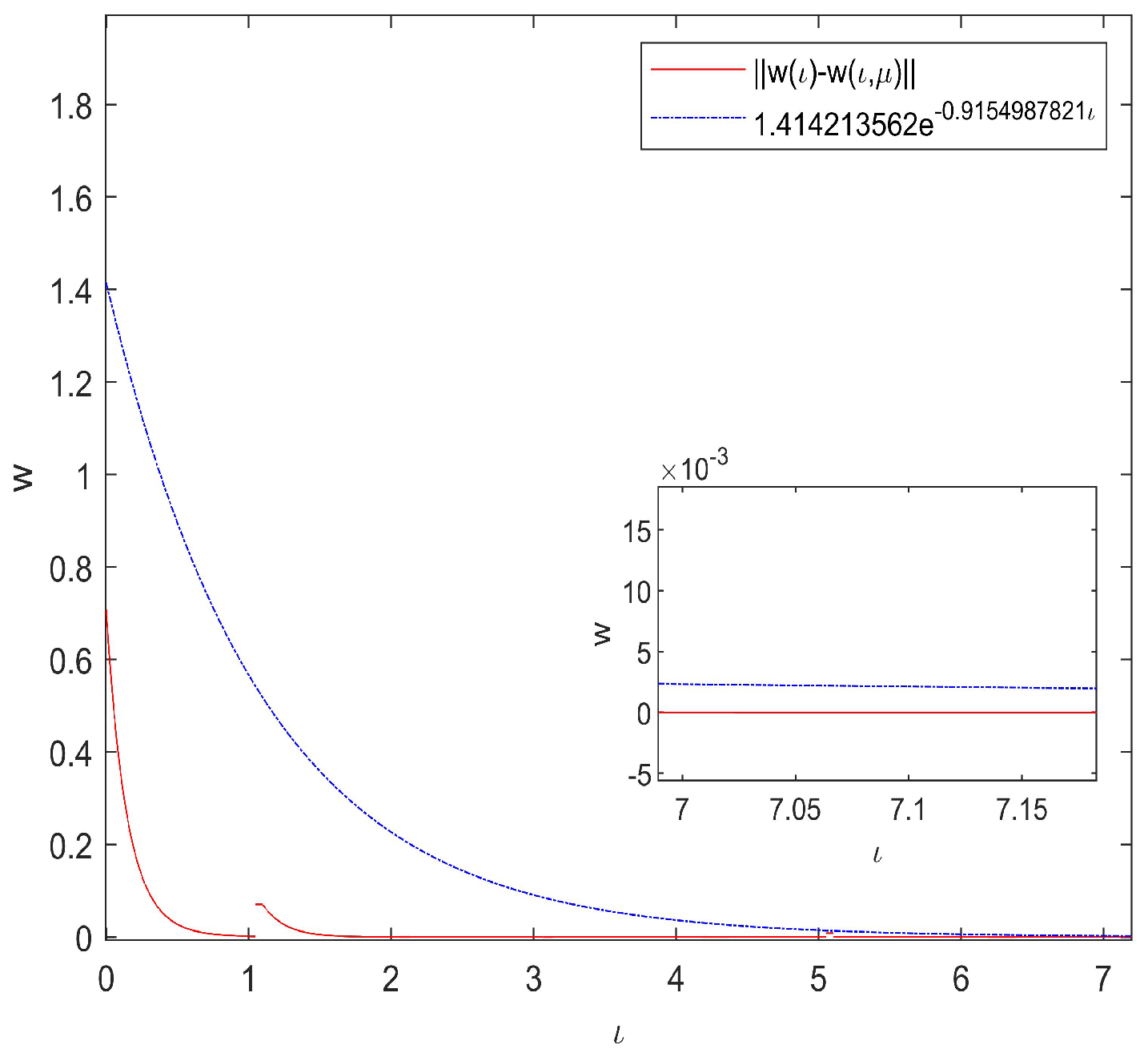
w ( ι ) w ( ι , μ ) Ξ w ( ι 0 ) w ( ι 0 , μ ) e ( N l n ( 1 + | μ | Ξ L 2 ) Y + | μ | Ξ L 1 ) ( ι ι 0 ) 1.414213562 e 0.9154987821 ι
by Theorem 3. Then, we represent (13) in Figure 4.

6. Conclusions

Differential equation models with impulses are usually established to study many phenomena in life [23,24,25,26]. We note that Stamova and Stamov [8] proposed a forced perturbed biological model with impulsive effects at fixed moments, which can be applied to blood models, drug models, and even predator–prey models. They gave the conditions for the existence of a unique AP solution and the exponential stability of the solution for this model. We are very interested in this work.
After careful reading, we introduced the non-instantaneous impulse factor into this model and proposed a forced perturbed non-instantaneous impulsive model. Then, we also provided conditions for the existence of a unique AP solution and the exponential stability of the solution for this model. As far as we know, this work is a generalization of previous works and has not been done before.
There are many limitations to our work. It is known to us that the time delays are inevitable [27]. Therefore, we will gradually consider the dynamic behavior of models with fixed delay, variable delay, single delay and multiple delay in future work. Beyond that, there are some problems that we will consider in the future. For example, are these results applicable to fractional-order differential equations models like [28]? Can we extend our model to the case with randomness like [29]? What will happen if periodic distributions/generalized functions are used?
In addition, we are concerned about the investigations of [30,31,32] and will study in our future work how to solve the differential problem they mentioned.

Author Contributions

The contributions of all authors (Rui Ma and Mengmeng Li) are equal. All the main results were developed together. All authors have read and agreed to the published version of the manuscript.

Funding

This work was supported by the National Natural Science Foundation of China (12201148) and Guizhou Provincial Science and Technology Projects (No.QKHJC-ZK[2022]YB069).

Data Availability Statement

Not applicable.

Conflicts of Interest

The authors declare no conflict of interest.

References

  1. Cushing, J.M. Integrodifferential Equations and Delay Models in Population Dynamics; Springer Science & Business Media: Berlin/Heidelberg, Germany, 2013. [Google Scholar]
  2. Feng, X.M.; Liu, L.L.; Zhang, F.Q. Dynamical behavior of SEIR-SVS epidemic models with nonlinear incidence and vaccination. Acta Math. Appl. Sin. Engl. Ser. 2022, 38, 282–303. [Google Scholar] [CrossRef]
  3. Liu, Z.; Yang, X.F. A linear uncertain pharmacokinetic model driven by Liu process. Appl. Math. Model. 2021, 89, 1881–1899. [Google Scholar] [CrossRef]
  4. Wang, J.R.; Fečkan, M.; Zhang, W.L. On the nonlocal boundary value problem of geophysical fluid flows. Z. Angew. Math. Phys. 2021, 72, 27. [Google Scholar] [CrossRef]
  5. Wang, C.; Agarwal, R.P.; O’Regan, D. Matrix measure on time scales and almost periodic analysis of the impulsive Lasota-Wazewska model with patch structure and forced perturbations. Math. Methods Appl. Sci. 2016, 39, 5651–5669. [Google Scholar] [CrossRef]
  6. Yan, Y.; Wang, K.H.; Gui, Z.J. Periodic solution of impulsive predator-prey model with stage structure for the prey undercrowding effect. J. Phys. Conf. Ser. 2021, 1903, 012032. [Google Scholar] [CrossRef]
  7. Cardinali, T.; Rubbioni, P. The controllability of an impulsive integro-differential process with nonlocal feedback controls. Appl. Math. Comput. 2019, 347, 29–39. [Google Scholar] [CrossRef]
  8. Stamova, I.; Stamov, G. Applied Impulsive Mathematical Models; Springer International Publishing: Berlin/Heidelberg, Germany, 2016. [Google Scholar]
  9. Hernández, E.; O’Regan, D.; Bená, M.A. On a new class of abstract integral equations and applications. Appl. Math. Comput. 2012, 219, 2271–2277. [Google Scholar] [CrossRef]
  10. Wang, J.R.; Fečkan, M. A general class of impulsive evolution equations. Topol. Methods Nonlinear Anal. 2015, 46, 915–933. [Google Scholar] [CrossRef]
  11. Wang, J.R.; Zhou, Y.; Lin, Z. On a new class of impulsive fractional differential equations. Appl. Math. Comput. 2014, 242, 649–657. [Google Scholar] [CrossRef]
  12. Wang, J.R.; Fečkan, M. Non-Instantaneous Impulsive Differential Equations; IOP: London, UK, 2018. [Google Scholar]
  13. Guan, Y.; Fečkan, M.; Wang, J.R. Periodic solutions and Hyers-Ulam stability of atmospheric Ekman flows. Discret. Contin. Dyn. Syst. 2021, 41, 1157–1176. [Google Scholar] [CrossRef]
  14. Li, M.M.; Wang, J.R.; O’Regan, D. Positive almost periodic solution for a noninstantaneous impulsive Lasota-Wazewska model. Bull. Iran. Math. Soc. 2019, 46, 851–864. [Google Scholar] [CrossRef]
  15. Chen, X.X. Almost periodic solutions of nonlinear delay population equation with feedback control. Nonlinear Anal. Real World Appl. 2007, 8, 62–72. [Google Scholar]
  16. Chen, X.X.; Chen, F.D. Almost-periodic solutions of a delay population equation with feedback control. Nonlinear Anal. Real World Appl. 2006, 7, 559–571. [Google Scholar]
  17. Huang, P.; Li, X.; Liu, B. Almost periodic solutions for an asymmetric oscillation. J. Differ. Equ. 2017, 263, 8916–8946. [Google Scholar] [CrossRef]
  18. Zhou, H.; Wang, W.; Yang, L. Stage-structured hematopoiesis model with delays in an almost periodic environment. Appl. Math. Lett. 2021, 120, 107336. [Google Scholar] [CrossRef]
  19. Samoilenko, A.M.; Perestyuk, N.A. Impulsive Differential Equations; World Scientific: Singapore, 1995. [Google Scholar]
  20. Stamova, I. Stability Analysis of Impulsive Functional Differential Equations; Walter de Gruyter: Berlin, Germany, 2009. [Google Scholar]
  21. Ma, R.; Wang, J.R.; Li, M.M. Almost periodic solutions for two non-instantaneous impulsive biological models. Qual. Theory Dyn. Syst. 2022, 21, 84. [Google Scholar] [CrossRef]
  22. Qin, Y. Integral and Discrete Inequalities and Their Applications; Birkhäuser: Berlin, Germany, 2016. [Google Scholar]
  23. Jiao, J.J.; Cai, S.H.; Li, L.M.; Zhang, Y.J. Dynamics of a predator-prey model with impulsive biological control and unilaterally impulsive diffusion. Adv. Differ. Equ. 2016, 2016, 1–19. [Google Scholar] [CrossRef]
  24. He, Z.L.; Li, C.D.; Chen, L.; Cao, Z.G. Dynamic behaviors of the FitzHugh-Nagumo neuron model with state-dependent impulsive effects. Neural Netw. 2020, 121, 497–511. [Google Scholar] [CrossRef]
  25. Xiang, J.; Zhang, J.S.; Zheng, R.Q.; Li, X.Y.; Li, M. NIDM: Network impulsive dynamics on multiplex biological network for disease-gene prediction. Brief. Bioinform. 2021, 22, bbab080. [Google Scholar] [CrossRef]
  26. Shao, Y.F. Dynamics of an impulsive stochastic predator-prey system with the Beddington-DeAngelis functional response. Axioms 2021, 10, 323. [Google Scholar] [CrossRef]
  27. Ji, X.R.; Lu, J.Q.; Jiang, B.X.; Shi, K.B. Distributed synchronization of delayed neural networks: Delay-Dependent hybrid impulsive control. IEEE Trans. Netw. Sci. Eng. 2021, 9, 634–647. [Google Scholar] [CrossRef]
  28. You, Z.L.; Fečkan, M.; Wang, J.R. Relative controllability of fractional delay differential equations via delayed perturbation of Mittag-Leffler functions. J. Comput. Appl. Math. 2020, 378, 112939. [Google Scholar] [CrossRef]
  29. Sathiyaraj, T.; Wang, J.R.; O’Regan, D. Controllability of stochastic nonlinear oscillating delay systems driven by the Rosenblatt distribution. Proc. R. Soc. Edinb. Sect. A Math. 2021, 151, 217–239. [Google Scholar] [CrossRef]
  30. Kim, S.Y.; Ji, W.Q.; Deng, S.L.; Ma, Y.B.; Rackauckas, C. Stiff neural ordinary differential equations, Chaos: An Interdisciplinary. J. Nonlinear Sci. 2021, 31, 093122. [Google Scholar]
  31. Ramos, H.; Rufai, M.A. An adaptive one-point second-derivative Lobatto-type hybrid method for solving efficiently differential systems. Int. J. Comput. Math. 2022, 99, 1687–1705. [Google Scholar] [CrossRef]
  32. Jódar, L.; Villanueva, R.J.; Arenas, A.J.; González, G.C. Nonstandard numerical methods for a mathematical model for influenza disease. Math. Comput. Simul. 2008, 79, 622–633. [Google Scholar] [CrossRef]
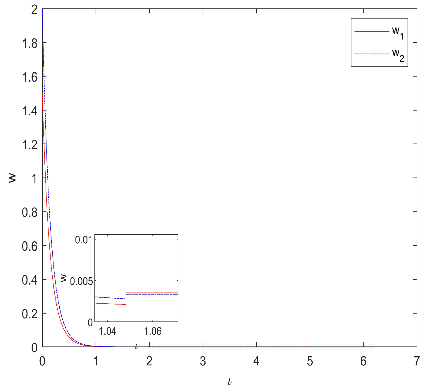
Figure 1. The positive almost periodic solution of model (8).
Axioms 11 00496 g001
Figure 2. The exponentially stable solution of model (8).
Axioms 11 00496 g002
Figure 3. The positive almost periodic solution of model (10).
Axioms 11 00496 g003
Figure 4. The exponentially stable solution of model (10).
Axioms 11 00496 g004
Publisher’s Note: MDPI stays neutral with regard to jurisdictional claims in published maps and institutional affiliations.