A Probabilistic Approach for Solutions of Deterministic PDE’s as Well as Their Finite Element Approximations

Abstract

A probabilistic approach is developed for the exact solution u to a deterministic partial differential equation as well as for its associated approximation $u_h^{(k)}$ performed by $P_k$ Lagrange finite element. Two limitations motivated our approach: On the one hand, the inability to determine the exact solution u relative to a given partial differential equation (which initially motivates one to approximating it) and, on the other hand, the existence of uncertainties associated with the numerical approximation $u_h^{(k)}$. We, thus, fill this knowledge gap by considering the exact solution u together with its corresponding approximation $u_h^{(k)}$ as random variables. By a method of consequence, any function where u and $u_h^{(k)}$ are involved are modeled as random variables as well. In this paper, we focus our analysis on a variational formulation defined on $W^{m,p}$ Sobolev spaces and the corresponding a priori estimates of the exact solution u and its approximation $u_h^{(k)}$ in order to consider their respective $W^{m,p}$-norm as a random variable, as well as the $W^{m,p}$ approximation error with regards to $P_k$ finite elements. This will enable us to derive a new probability distribution to evaluate the relative accuracy between two Lagrange finite elements $P_{k_1}$ and $P_{k_2},(k_1<k_2)$.

1. Introduction

We recently proposed new perspectives on relative finite element accuracy [1,2] by using a mixed geometrical-probabilistic interpretation of the error estimate in the case of finite element approximation (see for example [3] or [4]) derived from the Bramble–Hilbert lemma [5].

In [6], we further extended the results we had derived in the case of $H^1$ to Sobolev spaces $W^{m,p},(p\ne 2)$. To this end, we had to consider a more general framework, which mainly relied on the Banach–Nečas–Babusȟka $(\mathbf{BNB})$ abstract problem [7] devoted to Banach spaces.

This enabled us to obtain two new probability distributions that estimate the relative accuracy between two Lagrange finite elements $P_{k_1}$ and $P_{k_2}$, ($k_1<k_2$), by considering it as a random variable.

Thus, we obtained new results that show, among others, which of $P_{k_1}$ or $P_{k_2}$ is the most likely accurate, depending on the value of the mesh size h; this value is not considered anymore as proceeding towards zero, as in the standard procedure.

However, while obtaining these probability distributions, we only considered the standard error estimate dedicated to $P_k$ Lagrange finite elements, which approximates solution u to a variational problem $(\mathbf{BNB})$, u being formulated in the present case in Sobolev space $W^{m,p}(\Omega )$.

In the current study, we enrich the model published in [6] in multiple manners. Indeed, considering the functional framework $(\mathbf{BNB})$ in the case of the $W^{m,p}$ Sobolev spaces, we take into account the available a priori estimates one can deal with with respect to the solution of this kind of problem as well as for its approximation, together with the approximation error which corresponds to $P_k$ Lagrange finite elements (see Section 2.2). This will enable us to derive a new probabilistic model applied to the relative accuracy between two finite elements $P_{k_1}$ and $P_{k_2},(k_1<k_2)$. To this end, we also generalize the discrete probabilistic framework we considered in [1,6] by introducing continuous probabilistic formalism based on an appropriate density of probability (see Section 3.1).

The paper is organized as follows. In Section 2, we recall the mathematical problem we considered and introduce the basic definitions of functional tools to consider different estimations in $W^{m,p}$ Sobolev spaces. Section 3.1 is dedicated to the analysis of the relative finite elements accuracy based on a probabilistic approach. In Section 4, we detail the contribution of the a priori estimates and their interactions with the error estimate in the probability distributions we derived in Section 3.1. Concluding remarks follow.

2. The Functional and Approximation Frameworks and Their Corresponding Estimates

2.1. Abstract Problem in Banach Spaces and Corresponding Fundamental Results

In this section, we define an abstract framework that will enable us to consider the solution of a variational problem in Banach $W^{m,p}$ Sobolev spaces when $p\ne 2$ and its corresponding approximation computed by $P_k$ Lagrange finite elements.

In order to conduct this, we follow the presentation of A. Ern and J. L. Guermond [7], where two general Banach spaces W and V are involved where V is reflexive. We also recall the different assumptions needed in order to apply the $(\mathbf{BNB})$ Theorem valid in Banach spaces.

Let $u\in W$ be the solution of the variational formulation $(\mathbf{VP})$ defined by the following:

$$(\mathbf{VP})\left\{\begin{array}{c}\text{Find}u\in W\text{such that}:\hfill \\ a(u,v)=l(v),\forall v\in V,\hfill \end{array}\right.$$

(1)

where the following is the case:

• W and V are two Banach spaces equipped with norms denoted by ${\parallel .\parallel }_W$ and ${\parallel .\parallel }_V$, respectively; moreover, V is reflexive;
• a is a continuous bilinear form on $W\times V$, i.e, $a\in \mathcal{L}(W\times V;\mathbb{R}):$

  $$\forall (u,v)\in W\times V,|a(u,v)|\le {\parallel a\parallel }_{W,V}{\parallel u\parallel }_W{\parallel v\parallel }_V,$$

  with ${\displaystyle {\parallel a\parallel }_{W,V}\equiv inf\left\{C\in {\mathbb{R}}_{+}^{*},\forall (u,v)\in W\times V:|a(u,v)|\le {C\parallel u\parallel }_W{\parallel v\parallel }_V\right\}}$.;
• l is a continuous linear form on V, i.e, $l\in V^{\prime }=\mathcal{L}(V;\mathbb{R})$.

We further make the two following assumptions.

(BNB1)

$${\displaystyle \exists \alpha >0,\underset{w\in W}{inf}\underset{v\in V}{sup}\frac{a(w,v)}{{\parallel w\parallel }_W{\parallel v\parallel }_V}\ge \alpha ,}$$

(BNB2)

$$\forall v\in V,(\forall w\in W,a(w,v)=0)⟹(v=0).$$

Then, one can prove the (BNB) Theorem ([7], Theorem 2.6), which claims that the variational problem (VP) has one and only one solution in W and that the following a priori estimate holds.

$$\forall l\in V^{\prime }:{\parallel u\parallel }_W\le \frac{{\parallel l\parallel }_{V^{\prime }}}{\alpha }.$$

(2)

We also define the approximation $u_h^{(k)}$ of u solution to the approximate variational formulation:

$$(\mathbf{VP}{)}_h\left\{\begin{array}{c}\text{Find}{u}_h^{(k)}\in W_h^{(k)}\text{such that}:\hfill \\ a(u_h^{(k)},v_h^{(k)})=l(v_h^{(k)}),\forall v_h^{(k)}\in V_h^{(k)},\hfill \end{array}\right.$$

(3)

where we assume that $W_h^{(k)}$ and $V_h^{(k)}$ are two finite-dimensional subsets of W and V, respectively.

Moreover, as observed in [7] (Remark 2.23, p.92), neither condition (BNB1) nor condition (BNB2) imply its discrete counterpart. Then, the well-posedness of (3) is equivalent to the two following discrete conditions.

(BNB1_h)

$${\displaystyle \exists {\alpha }_h^{(k)}>0,\underset{w_h^{(k)}\in W_h^{(k)}}{inf}\underset{v_h^{(k)}\in V_h^{(k)}}{sup}\frac{a(w_h^{(k)},v_h^{(k)})}{\parallel w_h^{(k)}{\parallel }_{W_h^{(k)}}{\parallel v_h^{(k)}\parallel }_{V_h^{(k)}}}\ge {\alpha }_h^{(k)},}$$

(BNB2_h)

$$\forall v_h^{(k)}\in V_h^{(k)},(\forall w_h^{(k)}\in W_h^{(k)},a(w_h^{(k)},v_h^{(k)})=0)⟹(v_h^{(k)}=0).$$

If we further assume that $\text{dim}(W_h^{(k)})$ = $\text{dim}(V_h^{(k)})$, a direct application of Theorem 2.2 in [7] enables us to write the following a priori estimate.

$$\forall l\in V^{\prime }:{\parallel u_h^{(k)}\parallel }_{W_h}\le \frac{{\parallel l\parallel }_{V^{\prime }}}{{\alpha }_h^{(k)}}.$$

(4)

In the next section, we will apply these results to the particular case where the exact solution u belongs to $W^{m,p}$ Sobolev spaces and the approximation $u_h^{(k)}$ is computed by the help of $P_k$ Lagrange finite elements.

2.2. Application to $W^{m,p}$ Sobolev Spaces and the Corresponding Error Estimate

We introduce an open-bounded subset $\Omega \subset {\mathbb{R}}^n$ exactly recovered by a mesh ${\mathcal{T}}_h$ composed by $N_K$n-simplexes $K_{\mu },(1\le \mu \le N_K),$ which respect the classical rules of regular discretization (see, for example, [4] or [8]). Moreover, we denote by h the mesh size of ${\mathcal{T}}_h$ (the largest diameter in the mesh ${\mathcal{T}}_h$) and the space of polynomials defined on a given n-simplex $K_{\mu }$ of degree less than or equal to k ($k\ge$ 1) by $P_k(K_{\mu })$.

Henceforth, we assume that approximate spaces $W_h^{(k)}$ and $V_h^{(k)}$ satisfy $\text{dim}(W_h^{(k)})$ = $\text{dim}(V_h^{(k)})$ and that they are included in the space of functions defined on $\Omega$ and composed of polynomials belonging to $P_k(K_{\mu }),(1\le \mu \le N_K)$.

Finally, we also specify the functional framework of the abstract problem (VP) by introducing $W^{m,p}$ Sobolev spaces as follows.

For any integer $m\ge 1$ and any $1\le p\le +\infty$, we denote by $W^{m,p}(\Omega )$ the Sobolev space of (class of) real-valued functions that, together with all their partial distributional derivatives of order less or equal to m, belongs to $L^p(\Omega )$:

$${\displaystyle W^{m,p}(\Omega )=\left\{u\in L^p(\Omega )/\forall \alpha ,|\alpha |\le m,{\partial }^{\alpha }u\in L^p(\Omega )\right\},}$$

(5)

$\alpha =({\alpha }_1,{\alpha }_2,\dots ,{\alpha }_n)\in {\mathbb{N}}^n$ being a multi-index for which its length $|\alpha |$ is given by $|\alpha |={\alpha }_1+\cdots +{\alpha }_n$, and ${\partial }^{\alpha }u$ is the the partial derivative of order $|\alpha |$ defined by the following.

$${\displaystyle {\partial }^{\alpha }u\equiv \frac{{\partial }^{|\alpha |}u}{\partial x_1^{{\alpha }_1}\cdots \partial x_n^{{\alpha }_n}}.}$$

(6)

We also consider norm ${\parallel .\parallel }_{m,p,\Omega }$ and semi-norms ${|.|}_{l,p,\Omega }$, which are, respectively, defined by the following:

$${\displaystyle \forall u\in W^{m,p}{(\Omega ):\parallel u\parallel }_{m,p,\Omega }={\left(\sum _{|\alpha |\le m}{\parallel {\partial }^{\alpha }u\parallel }_{L^p}^p\right)}^{1/p},{|u|}_{l,p,\Omega }={\left(\sum _{|\alpha |=l}{\parallel {\partial }^{\alpha }u\parallel }_{L^p}^p\right)}^{1/p},0\le l\le m,}$$

(7)

where ${\parallel .\parallel }_{L^p}$ denotes the standard norm in $L^p(\Omega )$.

Then, in order to fulfill the conditions of the (BNB) Theorem, particularly so that W is a Banach space and V a reflexive one, in the sequel of the paper, the following definitions of spaces W and V hold:

$$W\equiv W^{m,p}(\Omega )\mathrm{and}V\equiv W^{m^{\prime },p^{\prime }}(\Omega ),$$

(8)

where m and $m^{\prime }$ are two non zero integers, and p and $p^{\prime }$ two real positive numbers that satisfy $p\ne 2$ and $p^{\prime }>1$ such that the following is the case.

$${\displaystyle \frac{1}{p}+\frac{1}{p^{\prime }}=1.}$$

(9)

Regarding these choices, Sobolev’s space $\left(W^{m,p}(\Omega ),{\parallel .\parallel }_{m,p,\Omega }\right)$ is a Banach space and $\left(W^{m^{\prime },p^{\prime }}(\Omega ),{\parallel .\parallel }_{m^{\prime },p^{\prime },\Omega }\right)$ is a reflexive one [9]. Moreover, we have: $W_h^{(k)}\subset W^{m,p}(\Omega )$ and $V_h^{(k)}\subset W^{m^{\prime },p^{\prime }}(\Omega )$.

We can now recall the $W^{m,p}$ a priori error estimate for $P_k$ Lagrange finite elements we derived in [6]:

$$\parallel u-u_h^{(k)}{\parallel }_{m,p,\Omega }\le {\mathcal{C}}_k{h}^{k+1-m}{|u|}_{k+1,p,\Omega },$$

(10)

where ${\mathcal{C}}_k$ is a positive constant independent of h.

Remark 1.

Since we noticed that $W_h^{(k)}$ is included in $W^{m,p}(\Omega )$, by considering for the topology of $W_h^{(k)}$ that was induced from $W^{m,p}(\Omega )$ thanks to the triangle inequality, (2)–(4) and (10) result in the following error estimate:

$$\parallel u-u_h^{(k)}{\parallel }_{m,p,\Omega }\le min\left(\left[\frac{1}{\alpha }+\frac{1}{{\alpha }_h^{(k)}}\right]{\parallel l\parallel }_{V^{\prime }},{\mathcal{C}}_k{h}^{k+1-m}{|u|}_{k+1,p,\Omega }\right),$$

(11)

where $V^{\prime }$ is the duality of $W^{m^{\prime },p^{\prime }}(\Omega )$.

As one can observe, the right-hand side of (11) contains ${\alpha }_h^{(k)}$ for which its dependency on h is usually unknown, except for particular cases. This is the reason why we will assume it is bounded from below by a positive constant δ independent of h:

$$\forall h>0,0<\delta \le {\alpha }_h^{(k)}.$$

This uniform boundedness property of ${\alpha }_h^{(k)}$, crucial to guaranteeing optimal error estimates [7], is valid in multiple cases (see Chapters 4 and 5 in [7] or [10]) but not systematically (see for example first-order PDEs in [7]).

Next, from (11), we obtain the following:

$$\parallel u-u_h^{(k)}{\parallel }_{m,p,\Omega }\le min\left(\frac{{\parallel l\parallel }_{V^{\prime }}}{{\alpha }^{*}},{\mathcal{C}}_k{h}^{k+1-m}{|u|}_{k+1,p,\Omega }\right),$$

(12)

where ${\displaystyle \frac{1}{{\alpha }^{*}}=\frac{1}{\alpha }+\frac{1}{\delta }}$.

In the sequel, we will denote by ${\beta }_k$ the following expression.

$${\beta }_k\equiv min\left(\frac{{\parallel l\parallel }_{V^{\prime }}}{{\alpha }^{*}},{\mathcal{C}}_k{h}^{k+1-m}{|u|}_{k+1,p,\Omega }\right).$$

(13)

Finally, we also observe that there exists a critical value ${\hslash }_k$ of h defined by the following:

$${\displaystyle {\hslash }_k\equiv {\left(\frac{{\parallel l\parallel }_{V^{\prime }}}{{\alpha }^{*}{\mathcal{C}}_k{|u|}_{k+1,p,\Omega }}\right)}^{\frac{1}{k+1-m}},}$$

(14)

such that the error estimate (12) can be split according to the following.

$$\parallel u-u_h^{(k)}{\parallel }_{m,p,\Omega }\le \left|\begin{array}{cc}{\displaystyle \frac{{\parallel l\parallel }_{V^{\prime }}}{{\alpha }^{*}},}\hfill & ifh\ge {\hslash }_k,\hfill \\ {\displaystyle {\mathcal{C}}_k{h}^{k+1-m}{|u|}_{k+1,p,\Omega },}\hfill & ifh\le {\hslash }_k.\hfill \end{array}\right.$$

(15)

Based on this error estimate, the following section is devoted to deriving a probabilistic model applied to the relative accuracy between two Lagrange finite elements $P_{k_1}$ and $P_{k_2},(k_1<k_2),$ when the mesh size h has a given and fixed value.

3. The Probabilistic Analysis of the Relative Finite Elements Accuracy

In [6], we proposed two probability distributions that enabled us to obtain an evaluation of the more likely $W^{m,p}$ accurate between two Lagrange finite elements $P_{k_1}$ and $P_{k_2}$, $(k_1<k_2)$. These distributions were essentially derived by considering the error estimate (10).

In the present paper, we generalize these probability distributions by introducing two new inputs, which are the following:

• The error estimate (10) is enriched by the a priori estimates (2) and (4) finally considers (15).
• The probabilistic approach we develop is an extension of those we considered in [1,6]. More precisely, by the help of an ad hoc density probability, we derive the probability distribution of a suitable random variable so that we can compare two approximation errors $\parallel u-u_h^{(k_1)}{\parallel }_{m,p,\Omega }$ and $\parallel u-u_h^{(k_2)}{\parallel }_{m,p,\Omega },(k_1<k_2)$, considered as random variables, as will be introduced now.

3.1. Random Solution and Random Approximations of Deterministic Partial Differential Equation

The purpose of this section is based of the following fundamental remark: the solution u to the variational problem (VP), except for particular cases, is totally unknown (being impossible to calculate it analytically); this motivates the numerical schemes one will choose to implement.

This inability to determine, in most cases, the exact solution u is mainly due to the complexity of the involved PDE’s operator; it indeed depends on complex combinations of integrals, partial derivatives and boundary conditions, as well as on the bent geometrical shape of the domain of integration $\Omega$. All of these ingredients hence participate in the incapability to analytically determine exact solution u as their relationship with u is inextricable and unknown.

As a consequence, this lack of knowledge and information regarding the dependency between these ingredients and solution u motivates us to consider u as a random variable, as well as any function of u. This paper is dedicated to the $W^{m,p}$ approximation error of $u-u_h^{(k)}$, considered as a random variable.

In this frame, we view solution u with respect to variational formulation (VP) defined by (1) in the same manner as it normally is viewed to consider the trajectory and contact point with the ground of any solid body that is thrown, i.e., as random. Indeed, in this case, due to the lack of information concerning the initial conditions of the trajectory of the body, the solution of the concerned inverse kinematic operator is inaccessible and is, thus, observed as a random variable.

In the case analyzed in this paper, the situation is much worse. Indeed, we investigate a general variational formulation (VP) where the analog of the inverse kinematic operator is too complex to enable us to analytically determine the corresponding solution of (VP) by any mathematical expression. It is one of the reasons that motivate us to view solution u and its approximation $u_h^{(k)}$ as random variables, since the corresponding approximate operator conserves the complexity of the original one described above.

3.2. The Probabilistic Distribution of the Relative Finite Elements Accuracy

In the previous section, we expressed the reason for why we consider solution u and its approximation $u_h^{(k)}$ as random variables.

In order to complete the description of the randomness feature of approximation error $\parallel u-u_h^{(k)}{\parallel }_{m,p,\Omega }$, we also remark that since the manner a given mesh grid generator will produce any mesh is random, the corresponding approximation $u_h^{(k)}$ is random too.

For all of these reasons, based on the error estimate (12) and (13), we can only affirm that the value of approximation error $\parallel u_h^{(k)}{-u\parallel }_{m,\Omega }$ is somewhere within interval $[0,{\beta }_k]$.

As a consequence, we decide to view norm $\parallel u-u_h^{(k)}{\parallel }_{m,p,\Omega }$ as a random variable defined as follows.

Let $k,m$ and p be fixed. We introduce the random variable $X_{m,p}^{(k)}$ defined by the following.

$$\begin{array}{}(16)& X_{m,p}^{(k)}:\hfill & \hfill W^{m,p}(\Omega )\times W_h^{(k)}& ⟶& [0,{\beta }_k]\hfill (17)& & \hfill \mathit{\omega }\equiv (u,u_h^{(k)})& ⟼& X_{m,p}^{(k)}(\mathit{\omega })=X_{m,p}^{(k)}(u,u_h^{(k)})={\parallel u-u_h^{(k)}\parallel }_{m,p,\Omega }.\hfill \end{array}$$

Thus, space product $W^{m,p}(\Omega )\times W_h^{(k)}$ plays the role of the usual probability space introduced in this context.

Now, regarding the absence of information concerning the more likely or less likely values of norm $\parallel u-u_h^{(k)}{\parallel }_{m,p,\Omega }$ within interval $[0,{\beta }_k]$, we assume that random variable $X_{m,p}^{(k)}$ is uniformly distributed over interval $[0,{\beta }_k]$ with the following meaning.

$$\forall (a,b)\in {\mathbb{R}}^2,0\le a<b\le {\beta }_k:Prob\left\{X_{m,p}^{(k)}\in [a,b]\right\}=\frac{b-a}{{\beta }_k}.$$

(18)

Equation (18) means that if one slides interval $[a,b]$ anywhere in $[0,{\beta }_k]$, the probability of event ${\displaystyle \left\{X_{m,p}^{(k)}\in [a,b]\right\}}$ does not depend on where interval $[a,b]$ is located in $[0,{\beta }_k]$, but only on its length; this corresponds to the property of uniformity of random variable $X_{m,p}^{(k)}$.

Let us now consider two families of Lagrange finite elements $P_{k_1}$ and $P_{k_2}$ corresponding to a set of values $(k_1,k_2)\in {\mathbb{N}}^2$ such that $0<k_1<k_2$.

The two corresponding inequalities given by (12) and (13), assuming that solution u to (VP) belong to $H^{k_2+1}(\Omega )$, are as follows:

$$\begin{array}{ccc}\hfill X_{m,p}^{(k_1)}\equiv {\parallel u-u_h^{(k_1)}\parallel }_{m,p,\Omega }& \le & {\beta }_{k_1},\hfill \end{array}$$

(19)

$$\begin{array}{ccc}\hfill X_{m,p}^{(k_2)}\equiv {\parallel u-u_h^{(k_2)}\parallel }_{m,p,\Omega }& \le & {\beta }_{k_2},\hfill \end{array}$$

(20)

where $u_h^{(k_1)}$ and $u_h^{(k_2)}$, respectively, denote $P_{k_1}$ and $P_{k_2}$ Lagrange finite element approximations of u and ${\beta }_{k_i},(i=1,2),$ as defined by (13).

Remark 2.

If one considers a given mesh for finite element $P_{k_2}$ that contains that of $P_{k_1}$, then for the particular class of problems where $(\mathbf{VP})$ is equivalent to a minimization formulation $(\mathbf{MP})$ (see for example [11]), one can show that the approximation error of the $P_{k_2}$ finite element is always smaller than that of $P_{k_1}$, and $P_{k_2}$ is more accurate than $P_{k_1}$ for all values of the mesh size h.

Therefore, in order to avoid this situation, for a given value of h, we consider two independent meshes built by a mesh generator for $P_{k_1}$ and $P_{k_2}$. Now, usually, in order to compare the accuracy between these two finite elements, one asymptotically considers inequalities (19) and (20) to conclude that, when h proceeds to zero, $P_{k_2}$ is more accurate than $P_{k_1}$, since $h^{k_2}$ proceeds faster to zero than $h^{k_1}$.

However, for a given application, h has a given and fixed value; thus, this method of comparison is not valid anymore. For this reason, our purpose is to determine the relative accuracy between two finite elements $P_{k_1}$ and $P_{k_2},(k_1<k_2)$ for a fixed value of h corresponding to two independent meshes.

Moreover, since we chose to consider two random variables $X_{m,p}^{(k_i)},(i=1,2),$ as uniformly distributed on their respective interval of values $[0,{\beta }_{k_i}],(i=1,2)$, we also assume that they are independent. This assumption is, once again, the result of the lack of information which led us to model the relationship between these two variables as independent, since any knowledge is available for more precisely localizing the value of $\parallel u-u_h^{(k_1)}{\parallel }_{m,p,\Omega }$ if the value of $\parallel u-u_h^{(k_2)}{\parallel }_{m,p,\Omega }$ was known and vice versa.

By the following result, we establish the density of probability of the random variable Z defined by the following: $Z=X_{m,p}^{(k_1)}-X_{m,p}^{(k_2)}$.

Theorem 1.

Let $X_{m,p}^{(k_i)},(i=1,2),$ be the two uniform and independent random variables defined by (16) and (17): $X_{m,p}^{(k_i)}\sim U([0,{\beta }_{k_i}])$, where ${\beta }_{k_i}$ is defined by (13).

Then, random variable Z defined on $\mathbb{R}$ has the following density of probability.

$$f_Z(z)=|\begin{array}{}(21)& \hfill 0& if& \left(z\le -{\beta }_{k_2}orz\ge {\beta }_{k_1}\right),\hfill (22)& \hfill \frac{{\beta }_{k_2}+z}{{\beta }_{k_1}{\beta }_{k_2}}& if& \left({\beta }_{k_1}\le {\beta }_{k_2}:-{\beta }_{k_2}\le z\le {\beta }_{k_1}-{\beta }_{k_2}\right)or\left({\beta }_{k_1}\ge {\beta }_{k_2}:-{\beta }_{k_2}\le z\le 0\right),\hfill (23)& \hfill \frac{1}{{\beta }_{k_2}}& if& \left({\beta }_{k_1}\le {\beta }_{k_2}:{\beta }_{k_1}-{\beta }_{k_2}\le z\le 0\right),\hfill (24)& \hfill \frac{1}{{\beta }_{k_1}}& if& \left({\beta }_{k_1}\ge {\beta }_{k_2}:0\le z\le {\beta }_{k_1}-{\beta }_{k_2}\right),\hfill (25)& \hfill \frac{{\beta }_{k_1}-z}{{\beta }_{k_1}{\beta }_{k_2}}& if& \left({\beta }_{k_1}\le {\beta }_{k_2}:0\le z\le {\beta }_{k_1}\right)or\left({\beta }_{k_1}\ge {\beta }_{k_2}:{\beta }_{k_1}-{\beta }_{k_2}\le z\le {\beta }_{k_1}\right).\hfill \end{array}$$

Proof. 

Let us now remark that since the support of two random variables $X_{m,p}^{(k_i)},$$(i=1,2),$ is $[0,{\beta }_{k_i}]$, the support of density $f_Z$ is, therefore, $[-{\beta }_{k_2},{\beta }_{k_1}]$, which corresponds to (21).

Let us consider the case where ${\beta }_{k_1}\le {\beta }_{k_2}$.

If $f_{X_{m,p}^{(k_i)}}(x_i)$ denotes the density of probability defined on $\mathbb{R}$ associated to each random variable $X_{m,p}^{(k_i)}$, since we assume that they are independent variables, density $f_Z(z)$ is given by the following:

$${\displaystyle f_Z(z)={\int }_{\mathbb{R}}{f}_{X_{m,p}^{(k_2)}}(x_2)f_{X_{m,p}^{(k_1)}}(x_2+z)d{x}_2,}$$

(26)

where

$${\displaystyle f_{X_{m,p}^{(k_i)}}(x_i)=\frac{1}{{\beta }_{k_i}}{\mathrm{𝟙}}_{[0,{\beta }_{k_i}]}(x_i),(i=1,2),}$$

(27)

and ${\mathrm{𝟙}}_{[c,d]}$ is the indicator function of the interval $[c,d],\forall (c,d)\in {\mathbb{R}}^2$.

Furthermore, due to the definition (27) of the density for each variable $X_{m,p}^{(k_i)},(i=1,2),$ the integrand of (26) can be expressed as follows:

$$f_{X_{m,p}^{(k_2)}}(x_2)f_{X_{m,p}^{(k_1)}}(x_2+z)=|\begin{array}{}(28)\hfill & \hfill \frac{1}{{\beta }_{k_1}{\beta }_{k_2}}& \mathrm{if}& 0\le x_2\le {\beta }_{k_2}\text{and}0\le x_2+z\le {\beta }_{k_1},\hfill (29)\hfill & \hfill 0& \mathrm{if}& \text{not}.\hfill \end{array}$$

As a consequence, $x_2\in [0,{\beta }_{k_2}]\cap [-z,-z+{\beta }_{k_1}]$, which leads one to consider the five following cases corresponding to the significant relative positions between intervals $[0,{\beta }_{k_2}]$ and $[-z,-z+{\beta }_{k_1}]$:

• Let us assume that $-z+{\beta }_{k_1}\le 0$. If $z\ge {\beta }_{k_1}$, then $[0,{\beta }_{k_2}]\cap [-z,-z+{\beta }_{k_1}]=⌀$ and $f_Z(z)=0$, which is again a result of (21);
• We consider now the values of z such that $-z\le 0$ and $0\le -z+{\beta }_{k_1}\le {\beta }_{k_2}$.
  If $0\le z\le {\beta }_{k_1}$, then $x_2\in [0,-z+{\beta }_{k_1}]$ and by (26) we obtain the expected expression of (25) since we have the following.

  $${\displaystyle f_Z(z)={\int }_0^{-z+{\beta }_{k_1}}\frac{d{x}_2}{{\beta }_{k_1}{\beta }_{k_2}}=\frac{{\beta }_{k_1}-z}{{\beta }_{k_1}{\beta }_{k_2}},(0\le z\le {\beta }_{k_1}).}$$

  (30)
• The following case concerns the values of z such that $-z\ge 0$ and $-z+{\beta }_{k_1}\le {\beta }_{k_2}$. If ${\beta }_{k_1}-{\beta }_{k_2}\le z\le 0$, then $x_2\in [-z,-z+{\beta }_{k_1}]$ and we obtain (23) since the following is the case.

  $${\displaystyle f_Z(z)={\int }_{-z}^{-z+{\beta }_{k_1}}\frac{d{x}_2}{{\beta }_{k_1}{\beta }_{k_2}}=\frac{1}{{\beta }_{k_2}},({\beta }_{k_1}-{\beta }_{k_2}\le z\le 0).}$$

  (31)
• If $-z\le 0$ and $-z+{\beta }_{k_1}\ge {\beta }_{k_2}$, then $0\le z\le {\beta }_{k_1}-{\beta }_{k_2}$, which is impossible since ${\beta }_{k_1}\le {\beta }_{k_2}$.
• We consider now the values of z such that $0\le -z\le {\beta }_{k_2}$ and $-z+{\beta }_{k_1}\ge {\beta }_{k_2}$.
  If $-{\beta }_{k_2}\le z\le {\beta }_{k_1}-{\beta }_{k_2}$, then $x_2\in [-z,{\beta }_{k_2}]$ and since we have the following:

  $${\displaystyle f_Z(z)={\int }_{-z}^{{\beta }_{k_2}}\frac{d{x}_2}{{\beta }_{k_1}{\beta }_{k_2}}=\frac{{\beta }_{k_2}+z}{{\beta }_{k_1}{\beta }_{k_2}},(-{\beta }_{k_2}\le z\le {\beta }_{k_1}-{\beta }_{k_2}),}$$

  (32)

  we obtain the expected expression of (22).
• Finally, if $-z\ge {\beta }_{k_2}$, then $[0,{\beta }_{k_2}]\cap [-z,-z+{\beta }_{k_1}]=⌀$ and $f_Z(z)=0$, which corresponds to (21).

The other cases corresponding to ${\beta }_{k_1}\ge {\beta }_{k_2}$ can be deduced by using the same arguments. □

From Theorem 1, one can infer the entire cumulative distribution function $F_Z(z)$ defined by the following.

$$F_Z(z)={\int }_{-\infty }^z{f}_Z(z)dz.$$

(33)

However, since we are interested in determining the more likely finite element between $P_{k_1}$ and $P_{k_2},(k_1<k_2)$, we focus the following corollary to the value of $F_Z(0)$, which corresponds to $Prob\left\{X_{m,p}^{(k_1)}\le X_{m,p}^{(k_2)}\right\}$.

Corollary 1.

Let $X_{m,p}^{(k_i)},(i=1,2),$ be the two uniform and independent random variables defined by (16)–(17): $X_{m,p}^{(k_i)}\sim U([0,{\beta }_{k_i}])$, where ${\beta }_{k_i}$ is defined by (13). Then, we have:

$$Prob\left\{X_{m,p}^{(k_1)}\le X_{m,p}^{(k_2)}\right\}=|\begin{array}{}(34)\hfill & \hfill 1-\frac{1}{2}\frac{{\beta }_{k_1}}{{\beta }_{k_2}}& if& {\beta }_{k_1}\le {\beta }_{k_2},\hfill (35)\hfill & \hfill \frac{1}{2}\frac{{\beta }_{k_2}}{{\beta }_{k_1}}& if& {\beta }_{k_1}\ge {\beta }_{k_2}.\hfill \end{array}$$

Proof. 

 

—

Let us consider the case where ${\beta }_{k_1}\le {\beta }_{k_2}$. Then, by definition (33) of the entire cumulative distribution function $F_Z(z)$, at $z=0$, we have the following:

$${\displaystyle F_Z(0)={\int }_{-\infty }^0{f}_Z(z)dz={\int }_{-{\beta }_{k_2}}^{{\beta }_{k_1}-{\beta }_{k_2}}\frac{{\beta }_{k_2}+z}{{\beta }_{k_1}{\beta }_{k_2}}dz+{\int }_{{\beta }_{k_1}-{\beta }_{k_2}}^0\frac{dz}{{\beta }_{k_2}}=1-\frac{1}{2}\frac{{\beta }_{k_1}}{{\beta }_{k_2}},}$$

(36)

where we used the values of the density $f_Z(z)$ given by (22) and (23).

—

In the same manner, when ${\beta }_{k_1}\ge {\beta }_{k_2}$, we have the following.

$${\displaystyle F_Z(0)={\int }_{-\infty }^0{f}_Z(z)dz={\int }_{-{\beta }_{k_2}}^0\frac{{\beta }_{k_2}+z}{{\beta }_{k_1}{\beta }_{k_2}}dz=\frac{1}{2}\frac{{\beta }_{k_2}}{{\beta }_{k_1}}.}$$

(37)

□

We can now explicate the probability distribution of event ${\displaystyle \left\{X_{m,p}^{(k_1)}\le X_{m,p}^{(k_2)}\right\}}$ given by (34) and (35) as a function of the mesh size h.

To this end, we remark that, since each ${\beta }_{k_i}(i=1,2)$ has two possible values depending on the relative position between h and ${\hslash }_{k_i}$ defined by (14), the probability distribution we are looking for must be splitted in the corresponding cases as well.

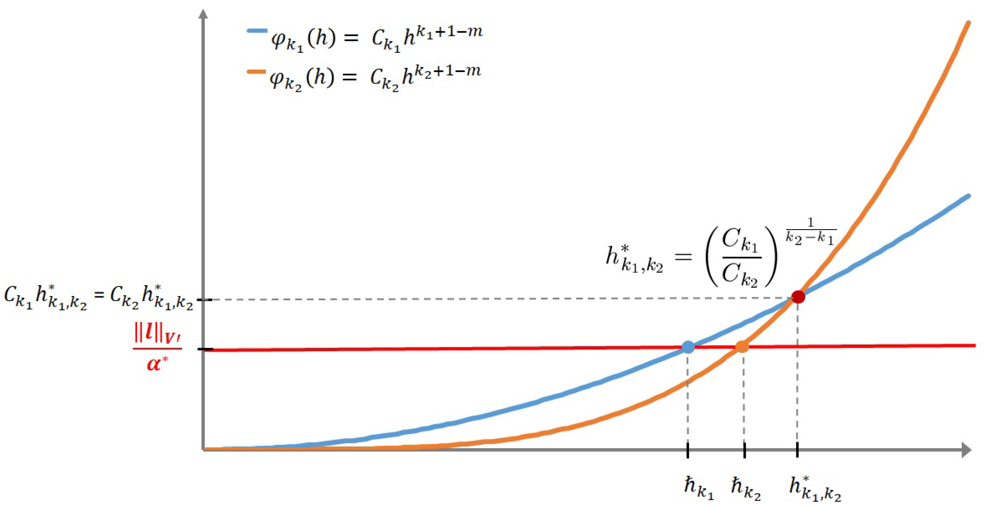
Let us, hence, introduce constants $C_{k_i},(i=1,2),$ defined by the following:

$$C_{k_i}={\mathcal{C}}_{k_i}{|u|}_{k_i+1,p,\Omega },$$

(38)

and the specific value $h_{k_1,k_2}^{*}$ of h which corresponds to the intersection of the curves ${\phi }_{k_i},(i=1,2),$ defined by ${\phi }_{k_i}(h)\equiv C_{k_i}{h}^{k_i+1-m}$ (see Figure 1).

Then, we have the following.

$${\displaystyle h_{k_1,k_2}^{*}={\left(\frac{C_{k_1}}{C_{k_2}}\right)}^{\frac{1}{k_2-k_1}}\equiv {\left(\frac{{\mathcal{C}}_{k_1}}{{\mathcal{C}}_{k_2}}\frac{{|u|}_{k_1+1,p,\Omega }}{{|u|}_{k_2+1,p,\Omega }}\right)}^{\frac{1}{k_2-k_1}}.}$$

(39)

We notice that $h_{k_1,k_2}^{*}$ and ${\hslash }_{k_i},(i=1,2),$ strongly depend on m and p, since ${\mathcal{C}}_{k_i}$ and ${\beta }_{k_i}$ depend on these two parameters as well. As a consequence, in the following theorem, the different formulas of $Prob\left\{X_{m,p}^{(k_1)}\le X_{m,p}^{(k_2)}\right\}$ will contain this dependency on m and p.

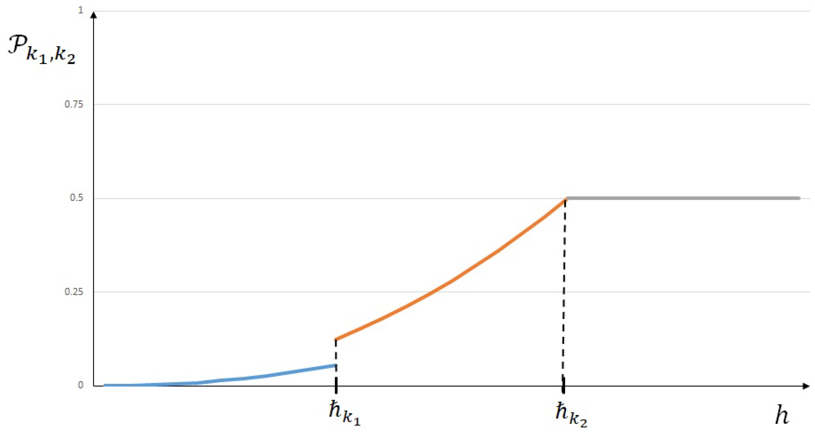
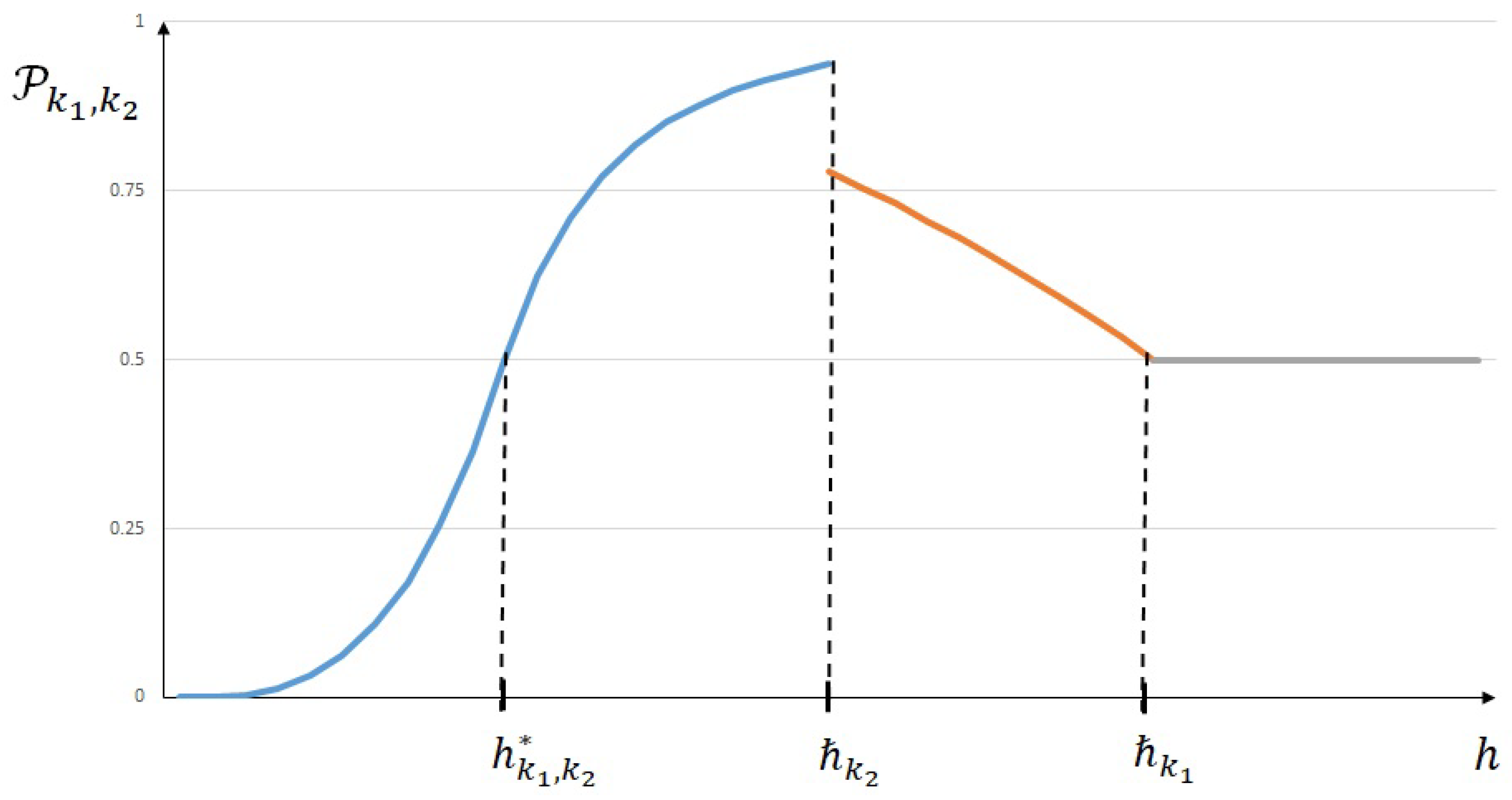
Theorem 2.

Let $X_{m,p}^{(k_i)},(i=1,2),$ be the two uniform and independent random variables defined by (16) and (17). Then, ${\displaystyle {\mathcal{P}}_{k_1,k_2}(h)\equiv Prob\left\{X_{m,p}^{(k_1)}\le X_{m,p}^{(k_2)}\right\}}$ is determined by the following.

If $h_{k_1,k_2}^{*}\ge max({\hslash }_{k_1},{\hslash }_{k_2})$, then ${\hslash }_{k_1}\le {\hslash }_{k_2}$ and we have:

$${\mathcal{P}}_{k_1,k_2}(h)=|\begin{array}{}(40)& \frac{1}{2}{\left(\frac{h}{h_{k_1,k_2}^{*}}\right)}^{k_2-k_1}\hfill & if& 0\le h\le {\hslash }_{k_1},\hfill (41)& \frac{1}{2}{\left(\frac{h}{{\hslash }_{k_2}}\right)}^{k_2+1-m}\hfill & if& {\hslash }_{k_1}\le h\le {\hslash }_{k_2},\hfill (42)& \frac{1}{2}& if& h\ge {\hslash }_{k_2}.\hfill \end{array}$$

If $h_{k_1,k_2}^{*}\le min({\hslash }_{k_1},{\hslash }_{k_2})$, then ${\hslash }_{k_2}\le {\hslash }_{k_1}$ and the following.

$${\mathcal{P}}_{k_1,k_2}(h)=|\begin{array}{}(43)& \frac{1}{2}{\left(\frac{h}{h_{k_1,k_2}^{*}}\right)}^{k_2-k_1}& if& 0\le h\le h_{k_1,k_2}^{*},\hfill (44)& 1-\frac{1}{2}{\left(\frac{h_{k_1,k_2}^{*}}{h}\right)}^{k_2-k_1}& if& h_{k_1,k_2}^{*}\le h\le {\hslash }_{k_2},\hfill (45)& 1-\frac{1}{2}{\left(\frac{h}{{\hslash }_{k_1}}\right)}^{k_1+1-m}& if& {\hslash }_{k_2}\le h\le {\hslash }_{k_1},\hfill (46)& \frac{1}{2}& if& h\ge {\hslash }_{k_1}.\hfill \end{array}$$

Proof. 

In order to establish the proof of Theorem 2, we will consider a geometrical interpretation of error estimate (19) and (20).

These two inequalities can indeed be geometrically viewed with the help of the relative position between the two curves ${\phi }_{k_i}(h),(i=1,2),$ introduced above and the horizontal line defined by ${\displaystyle \psi (h)\equiv \frac{{\parallel l\parallel }_{V^{\prime }}}{{\alpha }^{*}}}$ (see Figure 1).

Then, depending on the position of the horizontal line $\psi (h)$ with particular value $C_{k_i}{h}_{k_1,k_2}^{*},(i=1,2),$ we have to consider the two following cases:

—

If ${\displaystyle \frac{{\parallel l\parallel }_{V^{\prime }}}{{\alpha }^{*}}\le C_{k_1}{h}_{k_1,k_2}^{*}=C_{k_2}{h}_{k_1,k_2}^{*}}$, then ${\hslash }_{k_1}\le {\hslash }_{k_2}\le h_{k_1,k_2}^{*}$;

—

If ${\displaystyle \frac{{\parallel l\parallel }_{V^{\prime }}}{{\alpha }^{*}}\ge C_{k_1}{h}_{k_1,k_2}^{*}=C_{k_2}{h}_{k_1,k_2}^{*}}$, then $h_{k_1,k_2}^{*}\le {\hslash }_{k_2}\le {\hslash }_{k_1}$.

Thus, let us consider the first case when ${\displaystyle \frac{{\parallel l\parallel }_{V^{\prime }}}{{\alpha }^{*}}\le C_{k_1}{h}_{k_1,k_2}^{*}=C_{k_2}{h}_{k_1,k_2}^{*}}$ or equivalently $h_{k_1,k_2}^{*}\ge max({\hslash }_{k_1},{\hslash }_{k_2})$. Therefore, due to the relative positions between the three curves ${\phi }_{k_1},{\phi }_{k_2}$ and $\psi$, we have the following results:

• ${\displaystyle \forall h\le {\hslash }_{k_1}:C_{k_2}{h}^{k_2+1-m}\le C_{k_1}{h}^{k_1+1-m}\le \frac{{\parallel l\parallel }_{V^{\prime }}}{{\alpha }^{*}}}$ and ${\beta }_{k_2}\le {\beta }_{k_1}$ with ${\beta }_{k_i}=C_{k_i}{h}^{k_i+1-m},$$(i=1,2)$. Then, from (35), we obtain (40);
• ${\displaystyle \forall {\hslash }_{k_1}\le h\le {\hslash }_{k_2}:C_{k_2}{h}^{k_2+1-m}\le \frac{{\parallel l\parallel }_{V^{\prime }}}{{\alpha }^{*}}\le C_{k_1}{h}^{k_1+1-m}}$ and ${\beta }_{k_2}\le {\beta }_{k_1}$ with ${\displaystyle {\beta }_{k_1}=\frac{{\parallel l\parallel }_{V^{\prime }}}{{\alpha }^{*}}}$ and ${\beta }_{k_2}=C_{k_2}{h}^{k_2+1-m}$. Then, again from (35), we obtain (41);
• ${\displaystyle \forall {\hslash }_{k_2}\le h\le h_{k_1,k_2}^{*}:\frac{{\parallel l\parallel }_{V^{\prime }}}{{\alpha }^{*}}\le C_{k_2}{h}^{k_2+1-m}\le C_{k_1}{h}^{k_1+1-m}}$ and ${\displaystyle {\beta }_{k_1}={\beta }_{k_2}=\frac{{\parallel l\parallel }_{V^{\prime }}}{{\alpha }^{*}}}$. Then, from (34) or (35), we obtain (42);
• ${\displaystyle \forall h_{k_1,k_2}^{*}\le h:\frac{{\parallel l\parallel }_{V^{\prime }}}{{\alpha }^{*}}\le C_{k_1}{h}^{k_1+1-m}\le C_{k_2}{h}^{k_2+1-m}}$ and ${\displaystyle {\beta }_{k_1}={\beta }_{k_2}=\frac{{\parallel l\parallel }_{V^{\prime }}}{{\alpha }^{*}}}$. Then, again from (34) or (35), we also obtain (42).

We now consider the case where ${\displaystyle \frac{{\parallel l\parallel }_{V^{\prime }}}{{\alpha }^{*}}\ge C_{k_1}{h}_{k_1,k_2}^{*}=C_{k_2}{h}_{k_1,k_2}^{*}}$ which corresponds to $h_{k_1,k_2}^{*}\le min({\hslash }_{k_1},{\hslash }_{k_2})$. Therefore, using once again the relative positions between curves ${\phi }_{k_1},{\phi }_{k_2}$ and $\psi$, we deduce the following results:

• ${\displaystyle \forall h\le h_{k_1,k_2}^{*}:C_{k_2}{h}^{k_2+1-m}\le C_{k_1}{h}^{k_1+1-m}\le \frac{{\parallel l\parallel }_{V^{\prime }}}{{\alpha }^{*}}}$ and ${\beta }_{k_2}\le {\beta }_{k_1}$ with ${\beta }_{k_i}=C_{k_i}{h}^{k_i+1-m},$$(i=1,2)$. Then, from (35), we obtain (43);
• ${\displaystyle \forall h_{k_1,k_2}^{*}\le h\le {\hslash }_{k_2}:C_{k_1}{h}^{k_1+1-m}\le C_{k_2}{h}^{k_2+1-m}\le \frac{{\parallel l\parallel }_{V^{\prime }}}{{\alpha }^{*}}}$ and ${\beta }_{k_1}\le {\beta }_{k_2}$ with ${\beta }_{k_i}=C_{k_i}{h}^{k_i+1-m},(i=1,2)$. Then, from (34), we obtain (44);
• ${\displaystyle \forall {\hslash }_{k_2}\le h\le {\hslash }_{k_1}:C_{k_1}{h}^{k_1+1-m}\le \frac{{\parallel l\parallel }_{V^{\prime }}}{{\alpha }^{*}}\le C_{k_2}{h}^{k_2+1-m}}$ and ${\beta }_{k_1}\le {\beta }_{k_2}$ with ${\beta }_{k_1}=C_{k_1}{h}^{k_1+1-m}$ and ${\displaystyle {\beta }_{k_2}=\frac{{\parallel l\parallel }_{V^{\prime }}}{{\alpha }^{*}}}$. Then, again from (34), we obtain (45);
• ${\displaystyle \forall h\ge {\hslash }_{k_1}:\frac{{\parallel l\parallel }_{V^{\prime }}}{{\alpha }^{*}}\le C_{k_1}{h}^{k_1+1-m}\le C_{k_2}{h}^{k_2+1-m}}$ and ${\displaystyle {\beta }_{k_1}={\beta }_{k_2}=\frac{{\parallel l\parallel }_{V^{\prime }}}{{\alpha }^{*}}}$. Then, from (34) or (35), we obtain (46).

□

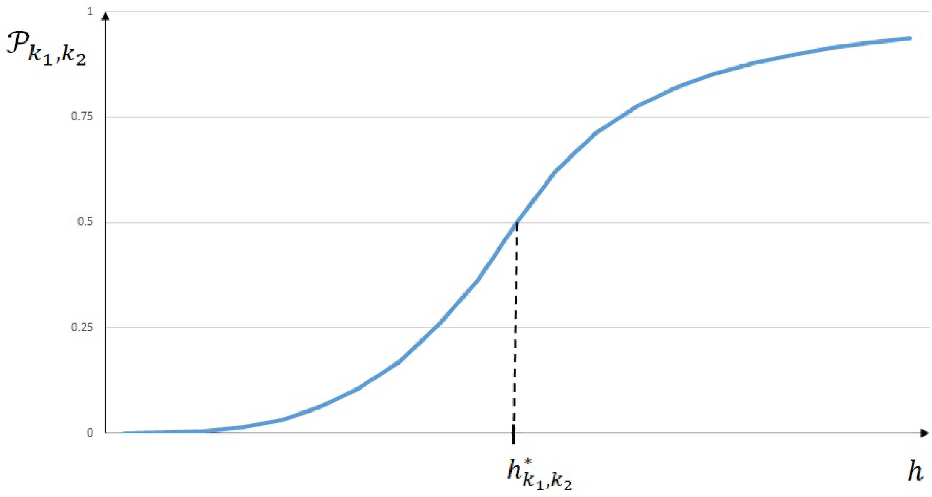
Remark 3.

We notice that the probability distribution ${\mathcal{P}}_{k_1,k_2}(h)$ given by Theorem 2 generalizes those that we found in [1,6]. Indeed, when we derived probability distribution ${\mathcal{P}}_{k_1,k_2}(h)$ without taking into account the a priori estimates (2) and (4), we obtained the following.

$${\mathcal{P}}_{k_1,k_2}(h)=|\begin{array}{}(47)& \hfill \frac{1}{2}{\left(\frac{h}{h_{k_1,k_2}^{*}}\right)}^{k_2-k_1}& if& 0\le h\le h_{k_1,k_2}^{*},\hfill (48)& \hfill 1-\frac{1}{2}{\left(\frac{h_{k_1,k_2}^{*}}{h}\right)}^{k_2-k_1}& if& h\ge h_{k_1,k_2}^{*}.\hfill \end{array}$$

In this case, we showed in [12] two numerical examples based on PDE’s formulation where exact solutions may be computed to illustrate probabilistic law (47) and (48).

In particular, we highlighted the statistical methodology that enabled us to determine a statistical estimator of the threshold $h_{k_1,k_2}^{*}$ given by (39).

Based on this study, one may adapt it in order to obtain applications that will illustrate the new probabilistic value we derived in Theorem 2.

Moreover, in Theorem 2, the contribution of a priori estimates (2) and (4) modifies the probability distribution given by (47) and (48), since the horizontal line ${\displaystyle \psi (h)=\frac{{\parallel l\parallel }_{V^{\prime }}}{{\alpha }^{*}}}$ interferes with the two polynomials $C_{k_i}{h}^{k_i+1-m},(i=1,2)$ (see Figure 1).

This phenomenon will be analyzed in the following section.

4. Discussion

First of all, let us plot the shape of the two cases of the probability distribution we derived in Theorem 2 and those we obtained in [1,6] that we recalled in (47) and (48).

As one can observe, the distribution (47) and (48) plotted in Figure 4 resembles more of the second case of Theorem 2 plotted in Figure 3 than its first case, as plotted in Figure 2.

In fact, in the latter case, when ${\hslash }_{k_1}\le {\hslash }_{k_2}$, line ${\displaystyle \psi (h)=\frac{{\parallel l\parallel }_{V^{\prime }}}{{\alpha }^{*}}}$ interacts with two polynomials $C_{k_i}{h}^{k_i+1-m},(i=1,2),$ before critical value $h_{k_1,k_2}^{*}$. As a consequence, its contribution correspondingly takes place in the expression of the probability distribution for $h\ge {\hslash }_{k_1}$.

On the contrary, when ${\hslash }_{k_1}\ge {\hslash }_{k_2}$, the contribution of line ${\displaystyle \psi (h)=\frac{{\parallel l\parallel }_{V^{\prime }}}{{\alpha }^{*}}}$ only has to be taken into account after the value of $h_{k_1,k_2}^{*}$. However, in this case, when $h\ge {\hslash }_{k_2}$, once again line $\psi (h)$ interacts with two polynomials $C_{k_i}{h}^{k_i+1-m},(i=1,2),$ and the equivalent distribution we found in (47) and (48) is cut to provide the corresponding one in (45) and (46) plotted in Figure 3.

This shows the importance of the a priori estimates (2) and (4), which are not considered in the classical point of view limited to the asymptotic behavior of error estimate (10), when the mesh size h proceeds to zero. The reason for this is the fact that the right hand sides of (2) and (4) do not depend on h; it does not bring any influence for the desired asymptotic behavior.

The goal of the probabilistic approach we developed in this paper is to evaluate, for any fixed value of the mesh size h, the relative accuracy between two Lagrange finite elements $P_{k_1}$ and $P_{k_2},(k_1\le k_2)$. The probability distributions of Theorem 2 adjust those that we had found in [1,6].

Indeed, probability distribution (47) and (48) claim that finite element $P_{k_1}$ is more likely to be accurate than $P_{k_2}$ with a high level of probability when $h\ge h_{k_1,k_2}^{*}$. Actually, this probability can reach the value of one, as it can be observed in Figure 4 and $P_{k_1}$ could be almost surely more accurate than $P_{k_2}$. Thus, distributions (40)–(42) and (43)–(46) limit the value of this probability.

More precisely, if ${\hslash }_{k_1}\le {\hslash }_{k_2}$, then the probability such that $P_{k_1}$ is more likely accurate than $P_{k_2}$ will never be greater than 0.5 (see Figure 2), and if ${\hslash }_{k_1}\ge {\hslash }_{k_2}$, then for $h\ge {\hslash }_{k_2}$ the corresponding probability will decrease to the limit value of 0.5, even if it increases with values greater than 0.5 for h values between $h_{k_1,k_2}^{*}$ and ${\hslash }_{k_2}$ (see Figure 3).

5. Conclusions

5.1. The Relative Accuracy between Two Finite Elements

In this paper, we presented a generalized probability distribution that takes into account the three available standard estimates one can confront with respect to solution u to a variational formulation together with its approximation $u_h^{(k)}$ performed by Lagrange finite elements $P_k$.

Those include the a priori estimates for solution u and its approximation $u_h^{(k)}$ carried out by finite elements, on the one hand, and the error estimate, on the other hand.

More precisely, by taking into account a priori estimates (2) and (4), we enriched probability distribution (47) and (48) that we obtained in [1,6] to find new ones (40)–(46), which were derived in Theorem 2.

As we observed in the previous paragraph, if the contribution of a priori estimates (2) and (4) are not considered when one limits the analysis of the relative accuracy between two finite elements to the asymptotic rate of convergence when the mesh size h proceeds to zero, one must deal with these two estimates in order to conclude about the more likely accurate one when h has a fixed value.

Moreover, regarding the probabilistic approach we developed in this paper, the a priori estimates (2) and (4) brought a more realistic behavior of distributions (40)–(46) in comparison with (47) and (48). Indeed, the probability given by (40)–(46) cannot reach a value of one since it was quite a surprise in (47) and (48) to obtain this theoretical value. This result meant that event “$P_{k_1}$ is more accurate than $P_{k_2}$” is an almost certain event when $k_1<k_2$.

5.2. Generalization to Other Numerical Methods

Finally, we would like to mention that the probabilistic approach we proposed in this study is not restricted to the finite elements method but may be extended to other types of approximation: given a class of numerical schemes and their corresponding approximation error estimates, one is able to order them not only in terms of asymptotic rate of convergence but also by evaluating the most probably accurate one.

It is, for example, the case of the numerical integration where the composite quadrature error has a mathematical structure, which looks similar to error estimate (10) we considered in the present study.

More precisely, as an example, for a composite quadrature of order k on a given interval $[a,b]$, if $f\in C^{k+1}([a,b])$ is a given function, the corresponding composite quadrature error can be written [13] as follows:

$${\displaystyle \left|{\int }_a^{b}f(x)dx-\sum _{i=0}^N{\lambda }_{i}f(x_i)\right|\le C_k{h}^{k+1},}$$

(49)

where h denotes the size of the equally spaced panels that discretized the interval $[a,b]$, $({\lambda }_i,x_i),(i=0,N),$ are $(2N+2)$ given numbers such that all $x_i$ belong to $[a,b]$, and $C_k$ is a constant independent of h that mainly depends on f and k.

As a consequence, due to the similar mathematical structure between (10) and (49), with the same arguments we introduced to compare the accuracy between two Lagrange finite elements $P_{k_1}$ and $P_{k_2},(k_1<k_2),$ one can evaluate the probability of the more accurate numerical composite quadrature associated to two different parameters $k_1$ and $k_2,(k_1\le k_2)$ for a fixed value of h.

This will make sense because, normally, to bypass the lack of information associated with the unknown value of the left hand side of (49) in interval $[0,C_k{h}^{k+1}]$, only the asymptotic convergence rate comparison is concerned for evaluating the relative accuracy between two numerical quadratures of order $k_1$ and $k_2,(k_1<k_2)$.

Nevertheless, this procedure is no longer available when one wants to compare two composite quadratures in the case when the size of the equally panels h is fixed, as it is for any application. Thus, the probabilistic approach we propose here could be a relevant alternative.

The same consideration may be developed in order to compare the accuracy between two numerical schemes of order $k_1$ and $k_2$, which are performed to approximate the exact solution of ordinary differential equations. To make precise these ideas, let us consider solution y of the first order ordinary differential initial value problem defined on a given interval $[t_0,t_0+T]$:

$$(\mathbf{CP})\left\{\begin{array}{ccc}{y}^{\prime }(t)\hfill & =\hfill & f(t,y(t)),t\in [t_0,t_0+T],\hfill \\ y(t_0)\hfill & =\hfill & y_0,\hfill \end{array}\right.$$

(50)

where $y_0$ is given.

Let us also restrict ourselves by considering one-step numerical methods to approximate function y solution to problem (CP).

Namely, if we introduce a constant mesh size $h=t_{n+1}-t_n$, where ${(t_n)}_{n=0,N}$ denotes the sequence of $(N+1)$ values of t within the interval $[t_0,t_0+T]$, then the corresponding one-step numerical scheme is given by the following:

$${(\mathbf{CP})}_h\left\{\begin{array}{ccc}{y}_{n+1}\hfill & =\hfill & y_n+h\Phi (t_n,y_n),n>0,\hfill \\ y_0\hfill & =\hfill & y_0,\hfill \end{array}\right.$$

(51)

where $\Phi$ is a given function “sufficiently” smooth that characterizes the numerical scheme (CP)_h.

Moreover, (CP)_h is called a numerical scheme of order k if [13]:

$${\displaystyle \sum _{n=0}^{N-1}|y(t_{n+1})-y(t_n)-h\Phi (t_n,y(t_n))|\le C_k{h}^k,}$$

(52)

where $C_k$ is a constant independent of h that depends on y, $\Phi$ and k (see [14] for the dependency on k).

Thus, when considering two one-step numerical methods of order $k_1$ and $k_2,(k_1<k_2),$ defined by two functions ${\Phi }_1$ and ${\Phi }_2$, and due to the similar structure between (10) and (52), one would be able to evaluate the probability of the more accurate scheme with the same arguments we implemented when comparing accuracy between $P_{k_1}$ and $P_{k_2}$ Lagrange finite elements.

In summary, when one wants to evaluate the relative accuracy between two numerical methods that belong to a given family of approximations, the probabilistic approach we propose in this study essentially depends on the ability to determine the constant $C_k$, which appears in different corresponding approximation errors (10), (49) or (52).

Indeed, for each of these errors of approximation, the complexity of the constant $C_k$ will suggest appropriate investigations. In the current study, we were devoted to the finite elements method, and we pointed out the important role of the a priori estimates (2) and (4), which are usually neglected, since they do not bring any asymptotic information/behavior when mesh size h proceeds to zero.

As a consequence, in order to render probability distribution (40)–(46) derived in Theorem 2, one will have to consider appropriate techniques that will make the determination (or at least the approximation) of different constants that are involved in (40)–(46) possible. This is mainly due to the contribution of the three estimates (2), (4) and (10), which results in (12), namely, ${\hslash }_{k_1},{\hslash }_{k_2}$ and $h_{k_1,k_2}^{*}$.

References

1. Chaskalovic, J.; Assous, F. A new probabilistic interpretation of Bramble-Hilbert lemma. Comput. Methods Appl. Math. 2019, 20, 79–87. [Google Scholar] [CrossRef] [Green Version]
2. Chaskalovic, J.; Assous, F. A new mixed functional-probabilistic approach for finite element accuracy. arXiv 2018, arXiv:1803.09552. [Google Scholar] [CrossRef]
3. Ciarlet, P.G. Basic error estimates for elliptic problems. In Handbook of Numerical Analysis; Ciarlet, P.G., Lions, J.L., Eds.; North Holland: Amsterdam, The Netherlands, 1991; Volume II. [Google Scholar]
4. Raviart, P.A.; Thomas, J.M. Introduction à L’analyse Numérique des Équations aux Dérivées Partielles; Masson: Issy-les-Moulineaux, France, 1982. [Google Scholar]
5. Bramble, J.H.; Hilbert, S.R. Estimation of linear functionals on Sobolev spaces with application to Fourier transforms and spline interpolation. SIAM J. Numer. Anal. 1970, 7, 112–124. [Google Scholar] [CrossRef]
6. Chaskalovic, J.; Assous, F. Explicit k-dependenc for Pk finite elements in Wm,p error estimates: Application to probability distributions for accuracy analysis. Appl. Anal. 2019, 100, 2825–2843. [Google Scholar] [CrossRef]
7. Ern, A.; Guermond, J.L. Theory and Practice of Finite Elements; Springer: New York, USA, 2004. [Google Scholar]
8. Ciarlet, P.G. The Finite Element Method for Elliptic Problems; Classics In Applied Mathematics; SIAM: Philadelphia, PA, USA, 2002. [Google Scholar]
9. Brezis, H. Analyse Fonctionnelle—Théorie et Applications; Masson: Paris, France, 1992. [Google Scholar]
10. Toundykov, D.; Avalos, G. A uniform discrete inf-sup inequality for finite element hydro-elastic models. Evol. Equ. Control Theory 2016, 5, 515–531. [Google Scholar] [CrossRef] [Green Version]
11. Chaskalovic, J. Mathematical and Numerical Methods for Partial Differential Equations; Springer: Basel, Switzerland, 2013. [Google Scholar]
12. Chaskalovic, J.; Assous, F. Numerical validation of probabilistic laws to evaluate finite element error estimates. Math. Model. Anal. 2021, 26, 684–694. [Google Scholar] [CrossRef]
13. Crouzeix, M.; Mignot, A.L. Analyse Numérique des Équations Diffécentielles; Masson: Issy-les-Moulineaux, France, 1984. [Google Scholar]
14. Stroud, A.H. Numerical Quadrature and Solution of Ordinary Differential Equations; Springer: Basel, Switzerland, 1974. [Google Scholar]
Figure 1. Relative positions between the curves C k i h k i + 1 m and the line l V / α * .
Axioms 10 00349 g001
Figure 2. Probability distribution P k 1 , k 2 ( h ) when h k 1 , k 2 * max ( k 1 , k 2 ) .
Axioms 10 00349 g002
Figure 3. Probability distribution P k 1 , k 2 ( h ) when h k 1 , k 2 * min ( k 1 , k 2 ) .
Axioms 10 00349 g003
Figure 4. Probability distribution P k 1 , k 2 ( h ) published in [1].
Axioms 10 00349 g004
Publisher’s Note: MDPI stays neutral with regard to jurisdictional claims in published maps and institutional affiliations.