Generalized Hypergeometric Function ₃F₂ Ratios and Branched Continued Fraction Expansions

Abstract

The paper is related to the classical problem of the rational approximation of analytic functions of one or several variables, particulary the issues that arise in the construction and studying of continued fraction expansions and their multidimensional generalizations—branched continued fraction expansions. We used combinations of three- and four-term recurrence relations of the generalized hypergeometric function ${}_3{F}_2$ to construct the branched continued fraction expansions of the ratios of this function. We also used the concept of correspondence and the research method to extend convergence, already known for a small region, to a larger region. As a result, we have established some convergence criteria for the expansions mentioned above. It is proved that the branched continued fraction expansions converges to the functions that are an analytic continuation of the ratios mentioned above in some region. The constructed expansions can approximate the solutions of certain differential equations and analytic functions, which are represented by generalized hypergeometric function ${}_3{F}_2.$ To illustrate this, we have given a few numerical experiments at the end.

1. Introduction

Questions that arise in economics, physics, biology, etc., lead to mathematical models, which are often formulated in the form of functional equations of various types, in particular, differential, integro-differential and difference equations (see, for example, [1,2,3,4,5,6,7]). One of the fundamental problems in approaches to finding solutions of such equations is the reconstruction of functions of one or several variables, as well as problems that arise in the development and implementation of effective methods and algorithms for representing and approximating the functions of one or several variables. There are many various tools for representing and approximating the above-mentioned functions, among which, perhaps, one of the most effective are continued fractions [8,9,10,11,12,13,14,15,16,17], and their multidimensional generalizations—branched continued fractions [18,19,20,21,22,23,24,25,26,27,28].

The concept of constructing continued fraction expansions of the ratios of hypergeometric functions was first introduced by C.F. Gauss in 1812 [29] as a composition of their three-term recurrence relations. This contributed to the construction and study of continued fraction expansions of many special functions, including those that are solutions of various differential equations (see more examples in ([8], Part III: Special Functions)).

The first branched continued fraction expansion for the Appell’s hypergeometric function $F_1$ proposed by N.S. Dronyuk in 1966 (see, ([21], pp. 244-252)). In a similarly way, using three- and four-term recurrence relations of the function $F_2$, its branched continued fraction expansions were constructed in [30]. Here also pointed out which three- and four-term recurrent relations give similar expansions for Appell’s hypergeometric function $F_4.$ Finally, the branched continued fraction expansions for function $F_3$ can be found in [31]. Note that the above-mentioned expansions have the same structure. The expansions of other structures were studied in [32] for Appell’s hypergeometric function $F_4,$ in [33,34] for Lauricella’s hypergeometric function $F_D,$ in [35] for Lauricella-Saran’s hypergeometric function $F_S,$ in [36] for Horn’s hypergeometric function $H_3.$ In the work [26], the branched continued fraction expansions were found for some ratios of generalized hypergeometric function ${}_r{F}_s$ and these results were generalized to the basic hypergeometric function ${}_r{\varphi }_s.$

We consider a generalized hypergeometric function

$${}_3{F}_2(\mathbf{a};\mathbf{b};z)={}_3{F}_2(a_1,a_2,a_3;b_1,b_2;z)=\sum _{n=0}^{\infty }\frac{{\left(a_1\right)}_n{\left(a_2\right)}_n{\left(a_3\right)}_n}{{\left(b_1\right)}_n{\left(b_2\right)}_n}\frac{z^n}{n!},$$

(1)

where $a_1,$$a_2,$$a_3,$$b_1,$ and $b_2$ are complex constants, $b_1,$$b_2$ are not equal to a non-positive integer, $z\in \mathbb{C},$${(·)}_k$ is the Pochhammer symbol defined for any complex number $\alpha$ and non-negative integer n by ${\left(\alpha \right)}_0=1$ and ${\left(\alpha \right)}_n=\alpha (\alpha +1)\dots (\alpha +n-1),$ which is the solution of differential equation (see, for example, ([37], p. 8))

$$z^3(1-z)\frac{d^{3}u}{d{z}^3}+z(a_{2}z-b_2)\frac{d^{2}u}{d{z}^2}+(a_{1}z-b_1)\frac{du}{dz}+a_{3}u=0,$$

(2)

where $u=u\left(z\right)$ is an unknown function of $z.$ It is know that the series (1) converges for all $\left|z\right|<1$ and that for $\left|z\right|=1$ its convergence depends on the parameters $a_1,$$a_2,$$a_3,$$b_1,$ and $b_2$ as follows:

(a)

if $\mathrm{Re}(b_1+b_2-a_1-a_1-a_3)>1,$ the series (1) converges for all $\left|z\right|=1;$

(b)

if $0<\mathrm{Re}(b_1+b_2-a_1-a_1-a_3)\le 1,$ the series (1) converges for $\left|z\right|=1$ and $z\ne 1;$

(c)

if $\mathrm{Re}(b_1+b_2-a_1-a_1-a_3)\le 0,$ the series (1) diverges for all $\left|z\right|=1.$

Note that in [26] the authors found, in particular, the branched continued expansions of three different types of ratios of generalized hypergeometric function:

$$\begin{array}{c}\frac{{}_3{F}_2(\mathbf{a};\mathbf{b};z)}{{}_3{F}_2(a_1,a_2,a_3+1;b_1,b_2+1;z)},\\ \frac{{}_3{F}_2(\mathbf{a};\mathbf{b};z)}{{}_3{F}_2(a_1,a_2,a_3+1;\mathbf{b};z)},\frac{{}_3{F}_2(\mathbf{a};\mathbf{b};z)}{{}_3{F}_2(\mathbf{a};b_1,b_2+1;z)}.\end{array}$$

(3)

In this paper, we construct and study the branched continued fraction expansions for four ratios of generalized hypergeometric function (1), among them two ratios of type (3), and two more of a new type. Explicit formulas for calculating the coefficients of constructed expansion by the coefficients of the function (1) will also be given. In Section 2.3, we derive some convergence criteria for the above-mentioned branched continued fractions and prove their convergence to functions, which are an analytic continuation of the ratios of generalized hypergeometric function ${}_3{F}_2$ in a certain region (here, region is an domain (open connected set) together with all, part or none of its boundary). Finally, we show an effective approximation of the analytic function, which under certain conditions is the solution of the differential Equation (2), using the constructed expansion.

2. Main Results

One of the problems in approaches to constructing branched continued fraction expansions for special functions of one or several variables (such as generalized hypergeometric functions, hypergeometric functions of Appell, Lauricella and Horn, etc.) is to obtain the simplest structure of branched continued fractions (elements of which are simple polynomials), as well as problems that arise in the development and implementation of effective methods for investigating the convergence of branched continued fractions.

Let us start with recurrence relations, which are the starting point in constructing the expansions of ratios of hypergeometric functions.

2.1. Recurrence Relations

It is know (see, for example, ([26], Lemma 14.1)) that for function (1) the following three-term recurrence relations hold

$$\begin{array}{c}{}_3{F}_2(\mathbf{a};\mathbf{b};z)={}_3{F}_2(a_1+1,a_2,a_3;b_1+1,b_2;z)-\frac{(b_1-a_1)a_2{a}_3}{(b_1+1)b_1{b}_2}z{}_3{F}_2(a_1+1,a_2+1,a_3+1;b_1+2,b_2+1;z),\end{array}$$

(4)

$$\begin{array}{c}{}_3{F}_2(\mathbf{a};\mathbf{b};z)={}_3{F}_2(a_1,a_2+1,a_3;b_1,b_2+1;z)-\frac{(b_2-a_2)a_1{a}_3}{(b_2+1)b_1{b}_2}z{}_3{F}_2(a_1+1,a_2+1,a_3+1;b_1+1,b_2+2;z),\end{array}$$

(5)

$$\begin{array}{c}{}_3{F}_2(\mathbf{a};\mathbf{b};z)={}_3{F}_2(a_1,a_2,a_3+1;b_1+1,b_2;z)-\frac{(b_1-a_3)a_1{a}_2}{(b_1+1)b_1{b}_2}z{}_3{F}_2(a_1+1,a_2+1,a_3+1;b_1+2,b_2+1;z),\end{array}$$

(6)

$$\begin{array}{c}{}_3{F}_2(\mathbf{a};\mathbf{b};z)={}_3{F}_2(a_1,a_2,a_3+1;b_1,b_2+1;z)-\frac{(b_2-a_3)a_1{a}_2}{(b_2+1)b_1{b}_2}z{}_3{F}_2(a_1+1,a_2+1,a_3+1;b_1+1,b_2+2;z).\end{array}$$

(7)

We note that these relations can be checked by direct verification.

Lemma 1.

The following four-term recurrence relations hold

$$\begin{array}{cc}\hfill {}_3{F}_2(\mathbf{a};\mathbf{b};z)& ={}_3{F}_2(a_1,a_2+1,a_3+1;b_1+1,b_2+1;z)-\frac{(b_1-a_3)a_1{a}_2}{(b_1+1)b_1{b}_2}z{}_3{F}_2(a_1+1,a_2+1,a_3+1;b_1+2,b_2+1;z)\hfill \end{array}$$

$$\begin{array}{cc}\hfill & -\frac{(b_2-a_2)(a_3+1)a_1}{(b_1+1)(b_2+1)b_2}z{}_3{F}_2(a_1+1,a_2+1,a_3+2;b_1+2,b_2+2;z),\hfill \\ \hfill {}_3{F}_2(\mathbf{a};\mathbf{b};z)& ={}_3{F}_2(a_1+1,a_2,a_3+1;b_1+1,b_2+1;z)-\frac{(b_2-a_3)a_1{a}_2}{(b_2+1)b_1{b}_2}z{}_3{F}_2(a_1+1,a_2+1,a_3+1;b_1+1,b_2+2;z)\hfill \end{array}$$

(8)

$$\begin{array}{cc}\hfill & -\frac{(b_1-a_1)(a_3+1)a_2}{(b_1+1)(b_2+1)b_2}z{}_3{F}_2(a_1+1,a_2+1,a_3+2;b_1+2,b_2+2;z).\hfill \end{array}$$

(9)

Proof. 

From the formula (5), replacing $a_3$ by $a_3+1$ and $b_1$ by $b_1+1,$ we get

$$\begin{array}{cc}\hfill {}_3{F}_2(a_1,a_2,a_3+1;b_1+1,b_2;z)& ={}_3{F}_2(a_1,a_2+1,a_3+1;b_1+1,b_2+1;z)\hfill \\ \hfill & -\frac{(b_2-a_2)a_1(a_3+1)}{(b_2+1)(b_1+1)b_2}z{}_3{F}_2(a_1+1,a_2+1,a_3+2;b_1+2,b_2+2;z).\hfill \end{array}$$

Applying this relation to the formula (6), we obtain the relation (8).

By analogy, combining the formulas (4) and (7), we have the relation (9). □

2.2. Expansions

In this subsection, we construct four closely related formal branched continued fraction expansions for the ratios of function (1).

Let ${\left(ij\right)}_0=(i_0,j_0)$ and

$$\mathcal{I}=\left\{\right(1,1);(1,2);(2,1);(2,2\left)\right\}.$$

Then, for each pair $(i_0,j_0)\in \mathcal{I}$ we set

$$R_{{\left(ij\right)}_0}(\mathbf{a};\mathbf{b};z)=\frac{{}_3{F}_2(\mathbf{a};\mathbf{b};z)}{{}_3{F}_2(a_1+{\delta }_{i_0}^1{\delta }_{j_0}^1+{\delta }_{i_0}^2{\delta }_{j_0}^2,a_2+{\delta }_{i_0}^1{\delta }_{j_0}^2+{\delta }_{i_0}^2{\delta }_{j_0}^1,a_3+{\delta }_{i_0}^2;b_1+{\delta }_{i_0}^1{\delta }_{j_0}^1+{\delta }_{i_0}^2,b_2+{\delta }_{i_0}^1{\delta }_{j_0}^2+{\delta }_{i_0}^2;z)},$$

(10)

where ${\delta }_k^p$ is the Kronecker symbol.

Applying the formula (4) to the relation (10) with $i_0=j_0=1$ one obtains

$$\begin{array}{cc}\hfill R_{1,1}(\mathbf{a};\mathbf{b};z)& =1-{\displaystyle \frac{(b_1-a_1)a_2{a}_3}{(b_1+1)b_1{b}_2}}z\frac{{}_3{F}_2(a_1+1,a_2+1,a_3+1;b_1+2,b_2+1;z)}{{}_3{F}_2(a_1+1,a_2,a_3;b_1+1,b_2;z)}\hfill \\ \hfill & =1-{\displaystyle \frac{(b_1-a_1)a_2{a}_3}{(b_1+1)b_1{b}_2}}z\frac{1}{R_{2,1}(a_1+1,a_2,a_3;b_1+1,b_2;z)}.\hfill \end{array}$$

(11)

By analogy, with the use of the formula (5) to (10) the following relation gives

$$R_{1,2}(\mathbf{a};\mathbf{b};z)=1-{\displaystyle \frac{(b_2-a_2)a_1{a}_3}{(b_2+1)b_1{b}_2}}z\frac{1}{R_{2,2}(a_1,a_2+1,a_3;b_1,b_2+1;z)}.$$

(12)

Dividing formula (8) by ${}_3{F}_2(a_1,a_2+1,a_3+1;b_1+1,b_2+1;z)$ we obtain

$$\begin{array}{cc}\hfill R_{2,1}(\mathbf{a};\mathbf{b};z)& =1-{\displaystyle \frac{(b_1-a_3)a_1{a}_2}{(b_1+1)b_1{b}_2}}z\frac{{}_3{F}_2(a_1+1,a_2+1,a_3+1;b_1+2,b_2+1;z)}{{}_3{F}_2(a_1,a_2+1,a_3+1;b_1+1,b_2+1;z)}\hfill \\ \hfill & -{\displaystyle \frac{(b_2-a_2)(a_3+1)a_1}{(b_1+1)(b_2+1)b_2}}z\frac{{}_3{F}_2(a_1+1,a_2+1,a_3+2;b_1+2,b_2+2;z)}{{}_3{F}_2(a_1,a_2+1,a_3+1;b_1+1,b_2+1;z)}\hfill \\ \hfill & =1-{\displaystyle \frac{(b_1-a_3)a_1{a}_2}{(b_1+1)b_1{b}_2}}z\frac{1}{R_{1,1}(a_1,a_2+1,a_3+1;b_1+1,b_2+1;z)}\hfill \\ \hfill & -{\displaystyle \frac{(b_2-a_2)(a_3+1)a_1}{(b_1+1)(b_2+1)b_2}}z\frac{1}{R_{2,2}(a_1,a_2+1,a_3+1;b_1+1,b_2+1;z)}.\hfill \end{array}$$

(13)

By analogy, dividing formula (9) by ${}_3{F}_2(a_1,a_2+1,a_3+1;b_1+1,b_2+1;z),$ the following relation gives

$$\begin{array}{cc}\hfill R_{2,2}(\mathbf{a};\mathbf{b};z)& =1-{\displaystyle \frac{(b_2-a_3)a_1{a}_2}{(b_2+1)b_1{b}_2}}z\frac{1}{R_{1,2}(a_1+1,a_2,a_3+1;b_1+1,b_2+1;z)}\hfill \\ \hfill & -{\displaystyle \frac{(b_1-a_1)(a_3+1)a_2}{(b_1+1)(b_2+1)b_1}}z\frac{1}{R_{2,1}(a_1+1,a_2,a_3+1;b_1+1,b_2+1;z)}.\hfill \end{array}$$

(14)

Now we combine formulas (11)–(14) into one. To this end, for each pair $(i_0,j_0)\in \mathcal{I}$ let us introduce the following set of multiindices

$${\mathcal{I}}_{{\left(ij\right)}_0}{=\{\left(ij\right)}_k:{\left(ij\right)}_k=(i_1,j_1,i_2,j_2,\dots ,i_k,j_k),1+{\delta }_{i_{k-1}}^1\le i_k\le 2,j_k\in \{1,2\},|i_k-j_k|\ne |i_{k-1}-j_{k-1}|,k\ge 1\}.$$

Then, for all $k\ge 1$ and for all ${\left(ij\right)}_k\in {\mathcal{I}}_{{\left(ij\right)}_0},$ ${\left(ij\right)}_0\in \mathcal{I}$ we set

$$\begin{array}{c}{\mathbf{a}}_{{\left(ij\right)}_k}^{{\left(ij\right)}_0}=\left(a_1+\sum _{p=0}^{k-1}({\delta }_{i_p}^1{\delta }_{j_p}^1+{\delta }_{i_p}^2{\delta }_{j_p}^2),a_2+\sum _{p=0}^{k-1}({\delta }_{i_p}^1{\delta }_{j_p}^2+{\delta }_{i_p}^2{\delta }_{j_p}^1),a_3+\sum _{p=0}^{k-1}{\delta }_{i_p}^2\right),\\ {\mathbf{b}}_{{\left(ij\right)}_k}^{{\left(ij\right)}_0}=\left(b_1+\sum _{p=0}^{k-1}({\delta }_{i_p}^1{\delta }_{j_p}^1+{\delta }_{i_p}^2),b_2+\sum _{p=0}^{k-1}({\delta }_{i_p}^1{\delta }_{j_p}^2+{\delta }_{i_p}^2)\right),\end{array}$$

and also we set

$$\begin{array}{c}{c}_{{\left(ij\right)}_k}^{{\left(ij\right)}_0}={\displaystyle \frac{(b_1-a_3+{\sum }_{p=0}^{k-2}{\delta }_{i_p}^1{\delta }_{j_p}^1)(a_1+{\sum }_{p=0}^{k-2}({\delta }_{i_p}^1{\delta }_{j_p}^1+{\delta }_{i_p}^2{\delta }_{j_p}^2))(a_2+{\sum }_{p=0}^{k-2}({\delta }_{i_p}^1{\delta }_{j_p}^2+{\delta }_{i_p}^2{\delta }_{j_p}^1))}{(b_1+1+{\sum }_{p=0}^{k-2}({\delta }_{i_p}^1{\delta }_{j_p}^1+{\delta }_{i_p}^2))(b_1+{\sum }_{p=0}^{k-2}({\delta }_{i_p}^1{\delta }_{j_p}^1+{\delta }_{i_p}^2))(b_2+{\sum }_{p=0}^{k-2}({\delta }_{i_p}^1{\delta }_{j_p}^2+{\delta }_{i_p}^2))}},\end{array}$$

(15)

if $i_{k-1}=2,$$j_{k-1}=i_k=j_k=1,$

$$\begin{array}{c}{c}_{{\left(ij\right)}_k}^{{\left(ij\right)}_0}={\displaystyle \frac{(b_2-a_3+{\sum }_{p=0}^{k-2}{\delta }_{i_p}^1{\delta }_{j_p}^2)(a_1+{\sum }_{p=0}^{k-2}({\delta }_{i_p}^1{\delta }_{j_p}^1+{\delta }_{i_p}^2{\delta }_{j_p}^2))(a_2+{\sum }_{p=0}^{k-2}({\delta }_{i_p}^1{\delta }_{j_p}^2+{\delta }_{i_p}^2{\delta }_{j_p}^1))}{(b_2+1+{\sum }_{p=0}^{k-2}({\delta }_{i_p}^1{\delta }_{j_p}^2+{\delta }_{i_p}^2))(b_1+{\sum }_{p=0}^{k-2}({\delta }_{i_p}^1{\delta }_{j_p}^1+{\delta }_{i_p}^2))(b_2+{\sum }_{p=0}^{k-2}({\delta }_{i_p}^1{\delta }_{j_p}^2+{\delta }_{i_p}^2))}},\end{array}$$

(16)

if $i_{k-1}=j_{k-1}=j_k=2,$$i_k=1,$

$$\begin{array}{c}{c}_{{\left(ij\right)}_k}^{{\left(ij\right)}_0}={\displaystyle \frac{(b_1-a_1+{\sum }_{p=0}^{k-2}{\delta }_{i_p}^2{\delta }_{j_p}^1)(a_2+{\sum }_{p=0}^{k-2}({\delta }_{i_p}^1{\delta }_{j_p}^2+{\delta }_{i_p}^2{\delta }_{j_p}^1))(a_3+{\sum }_{p=0}^{k-2}{\delta }_{i_p}^2)}{(b_1+1+{\sum }_{p=0}^{k-2}({\delta }_{i_p}^1{\delta }_{j_p}^1+{\delta }_{i_p}^2))(b_1+{\sum }_{p=0}^{k-2}({\delta }_{i_p}^1{\delta }_{j_p}^1+{\delta }_{i_p}^2))(b_2+{\sum }_{p=0}^{k-2}({\delta }_{i_p}^1{\delta }_{j_p}^2+{\delta }_{i_p}^2))}},\end{array}$$

(17)

if $i_{k-1}=j_{k-1}=j_k=1,$$i_k=2,$

$$\begin{array}{c}{c}_{{\left(ij\right)}_k}^{{\left(ij\right)}_0}={\displaystyle \frac{(b_1-a_1+{\sum }_{p=0}^{k-2}{\delta }_{i_p}^2{\delta }_{j_p}^1)(a_3+1+{\sum }_{p=0}^{k-2}{\delta }_{i_p}^2)(a_2+{\sum }_{p=0}^{k-2}({\delta }_{i_p}^1{\delta }_{j_p}^2+{\delta }_{i_p}^2{\delta }_{j_p}^1))}{(b_1+1+{\sum }_{p=0}^{k-2}({\delta }_{i_p}^1{\delta }_{j_p}^1+{\delta }_{i_p}^2))(b_2+1+{\sum }_{p=0}^{k-2}({\delta }_{i_p}^1{\delta }_{j_p}^2+{\delta }_{i_p}^2))(b_1+{\sum }_{p=0}^{k-2}({\delta }_{i_p}^1{\delta }_{j_p}^1+{\delta }_{i_p}^2))}},\end{array}$$

(18)

if $i_{k-1}=j_{k-1}=i_k=2,$$j_k=1,$

$$\begin{array}{c}{c}_{{\left(ij\right)}_k}^{{\left(ij\right)}_0}={\displaystyle \frac{(b_2-a_2+{\sum }_{p=0}^{k-2}{\delta }_{i_p}^2{\delta }_{j_p}^2)(a_1+{\sum }_{p=0}^{k-2}({\delta }_{i_p}^1{\delta }_{j_p}^1+{\delta }_{i_p}^2{\delta }_{j_p}^2))(a_3+{\sum }_{p=0}^{k-2}{\delta }_{i_p}^2)}{(b_2+1+{\sum }_{p=0}^{k-2}({\delta }_{i_p}^1{\delta }_{j_p}^2+{\delta }_{i_p}^2))(b_1+{\sum }_{p=0}^{k-2}({\delta }_{i_p}^1{\delta }_{j_p}^1+{\delta }_{i_p}^2))(b_2+{\sum }_{p=0}^{k-2}({\delta }_{i_p}^1{\delta }_{j_p}^2+{\delta }_{i_p}^2))}},\end{array}$$

(19)

if $i_{k-1}=1,$$j_{k-1}=i_k=j_k=2,$

$$\begin{array}{c}{c}_{{\left(ij\right)}_k}^{{\left(ij\right)}_0}={\displaystyle \frac{(b_2-a_2+{\sum }_{p=0}^{k-2}{\delta }_{i_p}^2{\delta }_{j_p}^2)(a_3+1+{\sum }_{p=0}^{k-2}{\delta }_{i_p}^2)(a_1+{\sum }_{p=0}^{k-2}({\delta }_{i_p}^1{\delta }_{j_p}^1+{\delta }_{i_p}^2{\delta }_{j_p}^2))}{(b_1+1+{\sum }_{p=0}^{k-2}({\delta }_{i_p}^1{\delta }_{j_p}^1+{\delta }_{i_p}^2))(b_2+1+{\sum }_{p=0}^{k-2}({\delta }_{i_p}^1{\delta }_{j_p}^2+{\delta }_{i_p}^2))(b_2+{\sum }_{p=0}^{k-2}({\delta }_{i_p}^1{\delta }_{j_p}^2+{\delta }_{i_p}^2))}},\end{array}$$

(20)

if $j_{k-1}=1,$$i_{k-1}=i_k=j_k=2.$

This allows us to write the relations (11)–(14) in the form

$$R_{{\left(ij\right)}_0}(\mathbf{a};\mathbf{b};z)=1-\sum _{\genfrac{}{}{0pt}{}{i_1=1+{\delta }_{i_0}^1}{|i_1-j_1|\ne |i_0-j_0|,j_1\in \{1,2\}}}^2\frac{c_{{\left(ij\right)}_1}^{{\left(ij\right)}_0}z}{R_{i_1,j_1}({\mathbf{a}}_{{\left(ij\right)}_1}^{{\left(ij\right)}_0};{\mathbf{b}}_{{\left(ij\right)}_1}^{{\left(ij\right)}_0};z)}\mathrm{for} \mathrm{all}{\left(ij\right)}_0\in \mathcal{I},$$

(21)

where $c_{{\left(ij\right)}_1}^{{\left(ij\right)}_0},$${\left(ij\right)}_1\in {\mathcal{I}}_{{\left(ij\right)}_0},$ ${\left(ij\right)}_0\in \mathcal{I},$ are defined by formulas (15)–(20) for $k=1.$

By analogy, it is clear that for any $k\ge 2$ and for any ${\left(ij\right)}_{k-1}\in {\mathcal{I}}_{{\left(ij\right)}_0},$${\left(ij\right)}_0\in \mathcal{I}$ the following recurrence relation holds

$$R_{i_{k-1},j_{k-1}}({\mathbf{a}}_{{\left(ij\right)}_{k-1}}^{{\left(ij\right)}_0};{\mathbf{b}}_{{\left(ij\right)}_{k-1}}^{{\left(ij\right)}_0};z)=1-\sum _{\genfrac{}{}{0pt}{}{i_k=1+{\delta }_{i_{k-1}}^1}{|i_k-j_k|\ne |i_{k-1}-j_{k-1}|,j_k\in \{1,2\}}}^2\frac{c_{{\left(ij\right)}_k}^{{\left(ij\right)}_0}z}{R_{i_k,j_k}({\mathbf{a}}_{{\left(ij\right)}_k}^{{\left(ij\right)}_0};{\mathbf{b}}_{{\left(ij\right)}_k}^{{\left(ij\right)}_0};z)},$$

(22)

where $c_{{\left(ij\right)}_k}^{{\left(ij\right)}_0},$${\left(ij\right)}_k\in {\mathcal{I}}_{{\left(ij\right)}_0},$ ${\left(ij\right)}_0\in \mathcal{I},$ are defined by formulas (15)–(20).

Next, we will construct branched continued fraction expansions for $R_{{\left(ij\right)}_0}(\mathbf{a};\mathbf{b};z)$ for all ${\left(ij\right)}_0\in \mathcal{I}.$ Let ${\left(ij\right)}_0$ be arbitrary pair from the set $\mathcal{I}.$ Then, substituting relation (22) at $k=2$ in formula (21) on the first step we obtain

$$R_{{\left(ij\right)}_0}(\mathbf{a};\mathbf{b};z)=1-\sum _{\genfrac{}{}{0pt}{}{i_1=1+{\delta }_{i_0}^1}{|i_1-j_1|\ne |i_0-j_0|,j_1\in \{1,2\}}}^2\frac{c_{{\left(ij\right)}_1}^{{\left(ij\right)}_0}z}{{\displaystyle 1-\sum _{\genfrac{}{}{0pt}{}{i_2=1+{\delta }_{i_1}^1}{|i_2-j_2|\ne |i_1-j_1|,j_2\in \{1,2\}}}^2{\displaystyle \frac{c_{{\left(ij\right)}_2}^{{\left(ij\right)}_0}z}{R_{i_2,j_2}({\mathbf{a}}_{{\left(ij\right)}_2}^{{\left(ij\right)}_0};{\mathbf{b}}_{{\left(ij\right)}_2}^{{\left(ij\right)}_0};z)}}}},$$

where $c_{{\left(ij\right)}_r}^{{\left(ij\right)}_0},$${\left(ij\right)}_r\in {\mathcal{I}}_{{\left(ij\right)}_0},$ $r=1,2,$ are defined by formulas (15)–(20).

Next, applying recurrence relation (22) after $(n-1)$ steps, we get

$$R_{{\left(ij\right)}_0}(\mathbf{a};\mathbf{b};z)=1-\sum _{\genfrac{}{}{0pt}{}{i_1=1+{\delta }_{i_0}^1}{|i_1-j_1|\ne |i_0-j_0|,j_1\in \{1,2\}}}^2\frac{c_{{\left(ij\right)}_1}^{{\left(ij\right)}_0}z}{1}\genfrac{}{}{0pt}{}{}{-}\dots \genfrac{}{}{0pt}{}{}{-}\sum _{\genfrac{}{}{0pt}{}{i_n=1+{\delta }_{i_{n-1}}^1}{|i_n-j_n|\ne |i_{n-1}-j_{n-1}|,j_n\in \{1,2\}}}^2\frac{c_{{\left(ij\right)}_n}^{{\left(ij\right)}_0}z}{R_{i_n,j_n}({\mathbf{a}}_{{\left(ij\right)}_n}^{{\left(ij\right)}_0};{\mathbf{b}}_{{\left(ij\right)}_n}^{{\left(ij\right)}_0};z)},$$

(23)

where $c_{{\left(ij\right)}_r}^{{\left(ij\right)}_0},$${\left(ij\right)}_r\in {\mathcal{I}}_{{\left(ij\right)}_0},$ $1\le r\le n,$ are defined by formulas (15)–(20). Note that here we used the more convenient notation of branched continued fraction, proposed by J.F.W. Herschel ([38], p. 148) following the example of H.H. Bürmann.

Finally, by the relation (22), one obtains

$$R_{{\left(ij\right)}_0}(\mathbf{a};\mathbf{b};z)\sim 1-\sum _{\genfrac{}{}{0pt}{}{i_1=1+{\delta }_{i_0}^1}{|i_1-j_1|\ne |i_0-j_0|,j_1\in \{1,2\}}}^2\frac{c_{{\left(ij\right)}_1}^{{\left(ij\right)}_0}z}{1}\genfrac{}{}{0pt}{}{}{-}\sum _{\genfrac{}{}{0pt}{}{i_2=1+{\delta }_{i_1}^1}{|i_2-j_2|\ne |i_1-j_1|,j_2\in \{1,2\}}}^2{\displaystyle \frac{c_{{\left(ij\right)}_2}^{{\left(ij\right)}_0}z}{1}}\genfrac{}{}{0pt}{}{}{-}\dots \genfrac{}{}{0pt}{}{}{-}\sum _{\genfrac{}{}{0pt}{}{i_k=1+{\delta }_{i_{k-1}}^1}{|i_k-j_k|\ne |i_{k-1}-j_{k-1}|,j_k\in \{1,2\}}}^2\frac{c_{{\left(ij\right)}_k}^{{\left(ij\right)}_0}z}{1}\genfrac{}{}{0pt}{}{}{-}\dots ,$$

(24)

where the symbol ∼ denotes a formal branched continued fraction expansion, the coefficients $c_{{\left(ij\right)}_k}^{{\left(ij\right)}_0},$ ${\left(ij\right)}_k\in {\mathcal{I}}_{{\left(ij\right)}_0},$ are defined by formulas (15)–(20).

Thus, in (24) for each pair $(i_0,j_0)\in \mathcal{I}$ we have a formal expansion, which is used to construct branched continued fraction. For example, for $R_{1,1}(\mathbf{a};\mathbf{b};z)$ we have the following formal expansion

$$1-{\displaystyle \frac{c_{2,1}^{1,1}z}{1-{\displaystyle \frac{c_{2,1,1,1}^{1,1}z}{1-{\displaystyle \frac{c_{2,1,1,1,2,1}^{1,1}z}{1-{\displaystyle \frac{c_{2,1,1,1,2,1,1,1}^{1,1}z}{1-{}_{\ddots }}}-{\displaystyle \frac{c_{2,1,1,1,2,1,2,2}^{1,1}z}{1-{}_{\ddots }}}}}}}-{\displaystyle \frac{c_{2,1,2,2}^{1,1}z}{1-{\displaystyle \frac{c_{2,1,2,2,1,2}^{1,1}z}{1-{\displaystyle \frac{c_{2,1,2,2,1,2,2,2}^{1,1}z}{1-{}_{\ddots }}}}}-{\displaystyle \frac{c_{2,1,2,2,2,1}^{1,1}z}{1-{\displaystyle \frac{c_{2,1,2,2,2,1,1,1}^{1,1}z}{1-{}_{\ddots }}}-{\displaystyle \frac{c_{2,1,2,2,2,1,2,2}^{1,1}z}{1-{}_{\ddots }}}}}}}}}.$$

(25)

We note one of the interesting properties of this branched continued fraction. To formulate it, we will give a few definitions ([18], p. 17).

The ratios $c_{{\left(ij\right)}_k}^{{\left(ij\right)}_0}z/1,$ ${\left(ij\right)}_k\in {\mathcal{I}}_{{\left(ij\right)}_0},$ are called the kth partial quotients, and the set of all kth quotients forms the kth floor on the branched continued fraction (25).

Proposition 1.

Let $Q_k$ be the numbers of all kth partial quotients of the kth floor of the branched continued fraction (25). Then the sequence $\left\{Q_k\right\}$ is a sequence of Fibonacci numbers starting from the third number.

Proof. 

In view on (11)–(14), the partial quotient in the corresponding ratio with first index equal to 1, generates one partial quotient on the next floor, and with an index equal to 2, generates two partial quotients.

Therefore, according to (11) on the first floor is only one partial quotient, which, in turn, according to (13) on the second floor generates two partial quotients.

Let $p_k$ and $q_k$ be the numbers of partial quotients of the kth floor of finite branched continued fraction (25), the denominators of which have ratios with the first index equal to 1 and 2, respectively. It is obvious that $p_1=0$ and $q_1=1.$ Then on kth floor we have $Q_k=p_k+q_k$ partial quotients. Each of the $p_k$ partial quotients generates one partial quotient with the first index equal to 2, and each of the $q_k$ partial quotients generates two partial quotients with the first index equal to 1 and 2 in the corresponding ratios in the denominators.

Thus, if $k\ge 2,$ then

$$p_{k+1}=q_{k}and{q}_{k+1}=p_k+q_k.$$

It follows that for $k\ge 2$

$$Q_{k+1}=p_{k+1}+q_{k+1}=p_k+q_k+q_k=Q_k+p_{k-1}+q_{k-1}=Q_k+Q_{k-1},$$

that proves this proposition. □

It is clear that the other three expansions in the right-hand side (24) also have similar properties.

2.3. Convergence

One of the fundamental problems of the study of branched continued fractions is the proving of their convergence. New methods were developed and applied in [39,40,41,42,43,44,45] to establish convergence criteria and in [46,47,48,49,50] to find estimates of convergence rate.

We will remind some concepts on the theory of branched continued fractions (see, for example, [18]).

Let here and further ${\left(ij\right)}_0$ be an arbitrary pair from the set $\mathcal{I}.$ Let ${}^n{Q}_{{\left(ij\right)}_k}^{{\left(ij\right)}_0}\left(z\right)$ denote the ’tails’ of branched continued fraction

$$1-\sum _{\genfrac{}{}{0pt}{}{i_1=1+{\delta }_{i_0}^1}{|i_1-j_1|\ne |i_0-j_0|,j_1\in \{1,2\}}}^2\frac{c_{{\left(ij\right)}_1}^{{\left(ij\right)}_0}z}{1}\genfrac{}{}{0pt}{}{}{-}\sum _{\genfrac{}{}{0pt}{}{i_2=1+{\delta }_{i_1}^1}{|i_2-j_2|\ne |i_1-j_1|,j_2\in \{1,2\}}}^2{\displaystyle \frac{c_{{\left(ij\right)}_2}^{{\left(ij\right)}_0}z}{1}}\genfrac{}{}{0pt}{}{}{-}\dots ,$$

(26)

that is

$${}^n{Q}_{{\left(ij\right)}_n}^{{\left(ij\right)}_0}\left(z\right)=1,{\left(ij\right)}_n\in {\mathcal{I}}_{{\left(ij\right)}_0},n\ge 1,$$

(27)

and

$${}^n{Q}_{{\left(ij\right)}_k}^{{\left(ij\right)}_0}\left(z\right)=1-\sum _{\genfrac{}{}{0pt}{}{i_{k+1}=1+{\delta }_{i_k}^1}{|i_{k+1}-j_{k+1}|\ne |i_k-j_k|,j_{k+1}\in \{1,2\}}}^2\frac{c_{{\left(ij\right)}_{k+1}}^{{\left(ij\right)}_0}z}{1}\genfrac{}{}{0pt}{}{}{-}\dots \genfrac{}{}{0pt}{}{}{-}\sum _{\genfrac{}{}{0pt}{}{i_n=1+{\delta }_{i_{n-1}}^1}{|i_n-j_n|\ne |i_{n-1}-j_{n-1}|,j_n\in \{1,2\}}}^2\frac{c_{{\left(ij\right)}_n}^{{\left(ij\right)}_0}z}{1},$$

(28)

where ${\left(ij\right)}_k\in \mathcal{I},$$1\le k\le n-1,$$n\ge 2.$ Then it is clear that the following recurrence relation holds

$${}^n{Q}_{{\left(ij\right)}_k}^{{\left(ij\right)}_0}\left(z\right)=1-\sum _{\genfrac{}{}{0pt}{}{i_{k+1}=1+{\delta }_{i_k}^1}{|i_{k+1}-j_{k+1}|\ne |i_k-j_k|,j_{k+1}\in \{1,2\}}}^2\frac{c_{{\left(ij\right)}_{k+1}}^{{\left(ij\right)}_0}z}{{}^n{Q}_{{\left(ij\right)}_{k+1}}^{{\left(ij\right)}_0}\left(z\right)},{\left(ij\right)}_k\in \mathcal{I},1\le k\le n-1,n\ge 2.$$

(29)

If $f_n$ denotes the nth approximant of (26), then

$$\begin{array}{cc}\hfill f_n^{{\left(ij\right)}_0}\left(z\right)& =1-\sum _{\genfrac{}{}{0pt}{}{i_1=1+{\delta }_{i_0}^1}{|i_1-j_1|\ne |i_0-j_0|,j_1\in \{1,2\}}}^2\frac{c_{{\left(ij\right)}_1}^{{\left(ij\right)}_0}z}{1}\genfrac{}{}{0pt}{}{}{-}\sum _{\genfrac{}{}{0pt}{}{i_2=1+{\delta }_{i_1}^1}{|i_2-j_2|\ne |i_1-j_1|,j_2\in \{1,2\}}}^2\frac{c_{{\left(ij\right)}_2}^{{\left(ij\right)}_0}z}{1}\genfrac{}{}{0pt}{}{}{-}\dots \genfrac{}{}{0pt}{}{}{-}\sum _{\genfrac{}{}{0pt}{}{i_n=1+{\delta }_{i_{n-1}}^1}{|i_n-j_n|\ne |i_{n-1}-j_{n-1}|,j_n\in \{1,2\}}}^2\frac{c_{{\left(ij\right)}_n}^{{\left(ij\right)}_0}z}{1}\hfill \\ & =1-\sum _{\genfrac{}{}{0pt}{}{i_1=1+{\delta }_{i_0}^1}{|i_1-j_1|\ne |i_0-j_0|,j_1\in \{1,2\}}}^2\frac{c_{{\left(ij\right)}_1}^{{\left(ij\right)}_0}z}{{}^n{Q}_{{\left(ij\right)}_1}^{{\left(ij\right)}_0}\left(z\right)},n\ge 1.\hfill \end{array}$$

The branched continued fraction (26) is said to converges at $z=z_0$ if its sequence of approximants $\left\{f_n^{{\left(ij\right)}_0}\left(z\right)\right\}$ converges, and

$$\underset{n\to \infty }{lim}{f}_n^{{\left(ij\right)}_0}\left(z\right)$$

is called its value.

The branched continued fraction (26), whose elements are functions in the certain domain $D,$$D\subset \mathbb{C},$ is called uniformly convergent on set $E,$$E\subset D,$ if its sequence of approximants $\left\{f_n^{{\left(ij\right)}_0}\left(z\right)\right\}$ converges uniformly on $E.$ When this occurs for an arbitrary set E such that $\overline{E}\subset D$ (here $\overline{E}$ is the closure of the set E) we say that the branched continued fraction converges uniformly on every compact subset of $D.$

We adopt the convention that a branched continued fraction (26) and all of its approximants have value 1 at $z=0.$

If ${}^n{Q}_{{\left(ij\right)}_k}^{{\left(ij\right)}_0}\left(z\right)\ne 0$ for all ${\left(ij\right)}_k\in \mathcal{I},$$1\le k\le n,$$n\ge 1,$ and for all z in the certain set $D,$$D\subset \mathbb{C},$ then for each $m>n\ge 1$ the following formula is valid (see ([18], p. 28))

$$\begin{array}{cc}\hfill f_m^{{\left(ij\right)}_0}\left(z\right)-f_n^{{\left(ij\right)}_0}\left(z\right)& ={(-1)}^n\sum _{\genfrac{}{}{0pt}{}{i_1=1+{\delta }_{i_0}^1}{|i_1-j_1|\ne |i_0-j_0|,j_1\in \{1,2\}}}^2\frac{c_{{\left(ij\right)}_1}^{{\left(ij\right)}_0}·(-z)}{{}^m{Q}_{{\left(ij\right)}_1}^{{\left(ij\right)}_0}\left(z\right)·{}^n{Q}_{{\left(ij\right)}_1}^{{\left(ij\right)}_0}\left(z\right)}\dots \sum _{\genfrac{}{}{0pt}{}{i_n=1+{\delta }_{i_{n-1}}^1}{|i_n-j_n|\ne |i_{n-1}-j_{n-1}|,j_n\in \{1,2\}}}^2\frac{c_{{\left(ij\right)}_n}^{{\left(ij\right)}_0}·(-z)}{{}^m{Q}_{{\left(ij\right)}_n}^{{\left(ij\right)}_0}\left(z\right)·{}^n{Q}_{{\left(ij\right)}_n}^{{\left(ij\right)}_0}\left(z\right)}\hfill \end{array}$$

$$\begin{array}{c}\hfill \times \sum _{\genfrac{}{}{0pt}{}{i_{n+1}=1+{\delta }_{i_n}^1}{|i_{n+1}-j_{n+1}|\ne |i_n-j_n|,j_{n+1}\in \{1,2\}}}^2\frac{c_{{\left(ij\right)}_{n+1}}^{{\left(ij\right)}_0}·(-z)}{{}^m{Q}_{{\left(ij\right)}_{n+1}}^{{\left(ij\right)}_0}\left(z\right)}.\end{array}$$

(30)

The following result is valid.

Theorem 1.

Let (26) be a branched continued fraction with $c_{{\left(ij\right)}_k}^{{\left(ij\right)}_0},$${\left(ij\right)}_k\in {\mathcal{I}}_{{\left(ij\right)}_0},$ defined by (15)–(20) and such that

$$b_r\ge a_r\ge 0,b_r\ge a_3\ge 0,b_r\ne 0,r=1,2.$$

(31)

Then:

(A) 

the branched continued fraction (26) converges to a finite value $f^{{\left(ij\right)}_0}\left(z\right)$ for each $z\in D,$ where

$$D=\{z\in \mathbb{R}:z\le 0\},$$

(32)

and it converges uniformly on every compact subset of $IntD$;

(B) 

if $f_n^{{\left(ij\right)}_0}\left(z\right)$ denotes the nth approximant of the branched continued fraction (26), then for each $z\in D$

$$|f^{{\left(ij\right)}_0}\left(z\right)-f_n^{{\left(ij\right)}_0}\left(z\right)|\le \frac{{\left(2\right|z\left|\right)}^{n+1}}{{\left(2\right|z|+1)}^n},n\ge 1.$$

Proof. 

We will find the upper bound of $|f_m^{{\left(ij\right)}_0}\left(z\right)-f_n^{{\left(ij\right)}_0}\left(z\right)|$ for $m>n\ge 1$ and $z\in D.$

From (15)–(20) it is clear that for each ${\left(ij\right)}_k\in {\mathcal{I}}_{{\left(ij\right)}_0}$ the coefficients $c_{{\left(ij\right)}_k}^{{\left(ij\right)}_0}$ of branched continued fraction (26) take non-negative values in the assumption of this theorem. And, consequently, in view of the formulas (27) and (28) it follows that

$${}^n{Q}_{{\left(ij\right)}_k}^{{\left(ij\right)}_0}\left(z\right)\ge 1 \mathrm{for} \mathrm{all}z\in D \mathrm{and} {\left(ij\right)}_k\in \mathcal{I},1\le k\le n,n\ge 1.$$

(33)

In addition, the following inequality holds

$$c_{{\left(ij\right)}_k}^{{\left(ij\right)}_0}\le 1 \mathrm{for} \mathrm{all} {\left(ij\right)}_k\in {\mathcal{I}}_{{\left(ij\right)}_0}.$$

(34)

Indeed, for any ${\left(ij\right)}_{k-1}\in {\mathcal{I}}_{{\left(ij\right)}_0}$ if $k>1$ and $i_{k-1}=2,$$j_{k-1}=i_k=j_k=1$ we have

$$\begin{array}{cc}\hfill b_1-a_3+\sum _{p=0}^{k-2}{\delta }_{i_p}^1{\delta }_{j_p}^1& \le b_1-a_3+\sum _{p=0}^{k-2}({\delta }_{i_p}^1{\delta }_{j_p}^1+{\delta }_{i_p}^2)\hfill \\ & \le b_1+\sum _{p=0}^{k-2}({\delta }_{i_p}^1{\delta }_{j_p}^1+{\delta }_{i_p}^2),\hfill \\ \hfill a_1+\sum _{p=0}^{k-2}({\delta }_{i_p}^1{\delta }_{j_p}^1+{\delta }_{i_p}^2{\delta }_{j_p}^2)& \le a_1+\sum _{p=0}^{k-2}({\delta }_{i_p}^1{\delta }_{j_p}^1+{\delta }_{i_p}^2)\hfill \\ & \le b_1+\sum _{p=0}^{k-2}({\delta }_{i_p}^1{\delta }_{j_p}^1+{\delta }_{i_p}^2),\hfill \\ \hfill a_2+\sum _{p=0}^{k-2}({\delta }_{i_p}^1{\delta }_{j_p}^2+{\delta }_{i_p}^2{\delta }_{j_p}^1)& \le a_2+\sum _{p=0}^{k-2}({\delta }_{i_p}^1{\delta }_{j_p}^2+{\delta }_{i_p}^2)\hfill \\ & \le b_2+\sum _{p=0}^{k-2}({\delta }_{i_p}^1{\delta }_{j_p}^2+{\delta }_{i_p}^2).\hfill \end{array}$$

In view of the formula (15), in this case it follows (34). Now, since

$$\begin{array}{cc}\hfill b_2-a_3+\sum _{p=0}^{k-2}{\delta }_{i_p}^1{\delta }_{j_p}^2& \le b_2-a_3+\sum _{p=0}^{k-2}({\delta }_{i_p}^1{\delta }_{j_p}^2+{\delta }_{i_p}^2)\hfill \\ & \le b_2+\sum _{p=0}^{k-2}({\delta }_{i_p}^1{\delta }_{j_p}^2+{\delta }_{i_p}^2),\hfill \end{array}$$

from (16) we get (34), when $i_{k-1}=j_{k-1}=j_k=2$ and $i_k=1.$ Finally, by analogy, we are convinced of the validity of inequality (34) in other cases (see formulas (17)–(20)).

From the inequality (33) it follows that ${}^n{Q}_{{\left(ij\right)}_k}^{{\left(ij\right)}_0}\left(z\right)\ne 0$ for all ${\left(ij\right)}_k\in \mathcal{I},$$1\le k\le n,$$n\ge 1,$ and $z\in D.$ Therefore, from (30) for each $m>n\ge 1$ and $z\in D$ we get

$$\begin{array}{cc}\hfill f_m^{{\left(ij\right)}_0}\left(z\right)-f_n^{{\left(ij\right)}_0}\left(z\right)& ={(-1)}^n\sum _{\genfrac{}{}{0pt}{}{i_1=1+{\delta }_{i_0}^1}{|i_1-j_1|\ne |i_0-j_0|,j_1\in \{1,2\}}}^2\frac{c_{{\left(ij\right)}_1}^{{\left(ij\right)}_0}·(-z)}{{}^r{Q}_{{\left(ij\right)}_1}^{{\left(ij\right)}_0}\left(z\right)}\dots \sum _{\genfrac{}{}{0pt}{}{i_n=1+{\delta }_{i_{n-1}}^1}{|i_n-j_n|\ne |i_{n-1}-j_{n-1}|,j_n\in \{1,2\}}}^2\frac{c_{{\left(ij\right)}_n}^{{\left(ij\right)}_0}·(-z)}{{}^n{Q}_{{\left(ij\right)}_{n-1}}^{{\left(ij\right)}_0}\left(z\right)·{}^n{Q}_{{\left(ij\right)}_n}^{{\left(ij\right)}_0}\left(z\right)}\hfill \end{array}$$

$$\begin{array}{c}\hfill \times \sum _{\genfrac{}{}{0pt}{}{i_{n+1}=1+{\delta }_{i_n}^1}{|i_{n+1}-j_{n+1}|\ne |i_n-j_n|,j_{n+1}\in \{1,2\}}}^2\frac{c_{{\left(ij\right)}_{n+1}}^{{\left(ij\right)}_0}·(-z)}{{}^m{Q}_{{\left(ij\right)}_n}^{{\left(ij\right)}_0}\left(z\right)·{}^m{Q}_{{\left(ij\right)}_{n+1}}^{{\left(ij\right)}_0}\left(z\right)},\end{array}$$

(35)

where $r=m,$ if n is even, and $r=n,$ if n is odd.

Next, using the inequality (34), for any $z\in D$ and $k\ge 1$ we have

$$\underset{{\left(ij\right)}_k\in {\mathcal{I}}_{{\left(ij\right)}_0}}{max}\sum _{\genfrac{}{}{0pt}{}{i_{k+1}=1+{\delta }_{i_k}^1}{|i_{k-1}-j_{k-1}|\ne |i_k-j_k|,j_{k+1}\in \{1,2\}}}^2{c}_{{\left(ij\right)}_{k+1}}^{{\left(ij\right)}_0}·(-z)\le 2\left|z\right|,$$

which by the relations (28) and (29) and the inequality (33), for any $r\ge k+1$ and ${\left(ij\right)}_k\in {\mathcal{I}}_{{\left(ij\right)}_0}$ gives us

$$\begin{array}{cc}\hfill \sum _{\genfrac{}{}{0pt}{}{i_{k+1}=1+{\delta }_{i_k}^1}{|i_{k+1}-j_{k+1}|\ne |i_k-j_k|,j_{k+1}\in \{1,2\}}}^2\frac{c_{{\left(ij\right)}_{k+1}}^{{\left(ij\right)}_0}·(-z)}{{}^r{Q}_{{\left(ij\right)}_{k+1}}^{{\left(ij\right)}_0}\left(z\right)·{}^r{Q}_{{\left(ij\right)}_k}^{{\left(ij\right)}_0}\left(z\right)}& \le \frac{{\displaystyle \sum _{\genfrac{}{}{0pt}{}{i_{k+1}=1+{\delta }_{i_k}^1}{|i_{k+1}-j_{k+1}|\ne |i_k-j_k|,j_{k+1}\in \{1,2\}}}^2{c}_{{\left(ij\right)}_{k+1}}^{{\left(ij\right)}_0}·(-z)}}{{\displaystyle 1+\sum _{\genfrac{}{}{0pt}{}{i_{k+1}=1+{\delta }_{i_k}^1}{|i_{k+1}-j_{k+1}|\ne |i_k-j_k|,j_{k+1}\in \{1,2\}}}^2{c}_{{\left(ij\right)}_{k+1}}^{{\left(ij\right)}_0}·(-z)}}\hfill \end{array}$$

$$\begin{array}{c}\hfill \le \frac{2\left|z\right|}{1+2\left|z\right|}.\end{array}$$

(36)

Now, by a successive application of inequality (36) and relations (33) and (34) to the formula (35), for any $m>n\ge 1$ and $z\in D$ we arrive at

$$\begin{array}{cc}\hfill |f_m^{{\left(ij\right)}_0}\left(z\right)-f_n^{{\left(ij\right)}_0}\left(z\right)|& \le {\left(\frac{2\left|z\right|}{1+2\left|z\right|}\right)}^n\sum _{\genfrac{}{}{0pt}{}{i_1=1+{\delta }_{i_0}^1}{|i_1-j_1|\ne |i_0-j_0|,j_1\in \{1,2\}}}^2\frac{c_{{\left(ij\right)}_1}^{{\left(ij\right)}_0}·\left|z\right|}{{}^r{Q}_{{\left(ij\right)}_1}^{{\left(ij\right)}_0}\left(z\right)}\hfill \\ & \le \frac{{\left(2\right|z\left|\right)}^{n+1}}{{(1+2|z\left|\right)}^n},\hfill \end{array}$$

where $r=m,$ if n is even, and $r=n,$ if n is odd. Hence, due to the arbitrariness of m and taking into account that for any fixed $z\in D$

$$\frac{{\left(2\right|z\left|\right)}^{n+1}}{{(1+2|z\left|\right)}^n}\to 0\mathrm{as}n\to \infty ,$$

it follows that the branched continued fraction (26) converges to a finite value $f^{{\left(ij\right)}_0}\left(z\right)$ for each $z\in D.$

Let K be an arbitrary compact subset of $IntD.$ Then there exists $M>0$ such that for any $m>n\ge 1$

$$|f_m^{{\left(ij\right)}_0}\left(z\right)-f_n^{{\left(ij\right)}_0}\left(z\right)|\le \frac{{\left(2M\right)}^{n+1}}{{(1+2M)}^n}\mathrm{for} \mathrm{all}z\in K.$$

In addition, if m and r are arbitrary natural numbers such that $m>r\ge n,$ then

$$|f_m^{{\left(ij\right)}_0}\left(z\right)-f_r^{{\left(ij\right)}_0}\left(z\right)|\le |f_m^{{\left(ij\right)}_0}\left(z\right)-f_n^{{\left(ij\right)}_0}\left(z\right)|+|f_r^{{\left(ij\right)}_0}\left(z\right)-f_n^{{\left(ij\right)}_0}\left(z\right)| \mathrm{for} \mathrm{all} z\in K.$$

Hence, taking into account that

$$\frac{{\left(2M\right)}^{n+1}}{{(1+2M)}^n}\to 0\mathrm{as}n\to \infty ,$$

it follows that the branched continued fraction (26) converges uniformly on every compact subset of $IntD.$

Finally, passing to the limit as $m\to \infty ,$ we obtain (B). □

Note that it follows from the proof of Theorem 1 that (26) is a branched continued fraction with positive elements for each nonzero $z=z_0$ from the set (32). This means that (see, ([18], p. 29))

$$f_{2n-2}^{{\left(ij\right)}_0}\left(z_0\right)<f_{2n}^{{\left(ij\right)}_0}\left(z_0\right)<f_{2n+1}^{{\left(ij\right)}_0}\left(z_0\right)<f_{2n-1}^{{\left(ij\right)}_0}\left(z_0\right), n\ge 1,$$

(here $f_0^{{\left(ij\right)}_0}\left(z_0\right)=1$), so that the even and odd parts of (26) both converge to finite value $f^{{\left(ij\right)}_0}\left(z_0\right).$ This system of inequalities expresses a so-called ‘fork property’ for branched continued fractions.

Theorem 2.

Let (1) be a generalized hypergeometric function ${}_3{F}_2(\mathbf{a};\mathbf{b};z)$ with parameters satisfying the inequalities (31).

Then:

(A) 

for each $z\in H_{\epsilon },$ where

$$\begin{array}{c}{H}_{\epsilon }=\bigcup _{-\pi /(2+2\epsilon )<\phi <\pi /(2+2\epsilon )}{H}_{\phi ,\epsilon },\end{array}$$

(37)

$$\begin{array}{c}{H}_{\phi ,\epsilon }=\left\{z\in \mathbb{C}:\left|z\right|+\mathrm{Re}\left(z{e}^{-2i\phi }\right)\le \frac{1-\epsilon }{4}{cos}^2\phi \right\},0<\epsilon <1,\end{array}$$

(38)

the branched continued fraction (26), where $c_{{\left(ij\right)}_k}^{{\left(ij\right)}_0},$${\left(ij\right)}_k\in {\mathcal{I}}_{{\left(ij\right)}_0},$ defined by (15)–(20), converges to a finite value $f^{{\left(ij\right)}_0}\left(z\right)$;

(B) 

the convergence is uniform on every compact subset of $Int{H}_{\epsilon },$ and $f^{{\left(ij\right)}_0}\left(z\right)$ is holomorphic on $Int{H}_{\epsilon }$;

(C) 

the function $f^{{\left(ij\right)}_0}\left(z\right)$ is an analytic continuation of (10) in $H_{\epsilon }.$

In our proof we will use the auxiliary lemma, which follows from ([51], Theorem 2).

Lemma 2.

Let the elements $d_{{\left(ij\right)}_k}^{{\left(ij\right)}_0},$ ${\left(ij\right)}_k\in {\mathcal{I}}_{{\left(ij\right)}_0},$ of branched continued fraction

$$\sum _{\genfrac{}{}{0pt}{}{i_1=1+{\delta }_{i_0}^1}{|i_1-j_1|\ne |i_0-j_0|,j_1\in \{1,2\}}}^2\frac{d_{{\left(ij\right)}_1}^{{\left(ij\right)}_0}}{1}\genfrac{}{}{0pt}{}{}{-}\sum _{\genfrac{}{}{0pt}{}{i_2=1+{\delta }_{i_1}^1}{|i_2-j_2|\ne |i_1-j_1|,j_2\in \{1,2\}}}^2{\displaystyle \frac{d_{{\left(ij\right)}_2}^{{\left(ij\right)}_0}}{1}}\genfrac{}{}{0pt}{}{}{-}\dots$$

(39)

satisfy the following conditions

$$\sum _{\genfrac{}{}{0pt}{}{i_k=1+{\delta }_{i_{k-1}}^1}{|i_k-j_k|\ne |i_{k-1}-j_{k-1}|,j_k\in \{1,2\}}}^2\frac{|d_{{\left(ij\right)}_k}^{{\left(ij\right)}_0}|-Re\left(d_{{\left(ij\right)}_k}^{{\left(ij\right)}_0}{e}^{-i({\phi }_{{\left(ij\right)}_{k-1}}+{\phi }_{{\left(ij\right)}_k})}\right)}{p_{{\left(ij\right)}_{k-1}}(cos{\phi }_{{\left(ij\right)}_k}-p_{{\left(ij\right)}_k})}\le 2(1-\epsilon ),{\left(ij\right)}_k\in {\mathcal{I}}_{{\left(ij\right)}_0},$$

where ${\phi }_{{\left(ij\right)}_0},$$p_{{\left(ij\right)}_0},$ and ${\phi }_{{\left(ij\right)}_k},$ $p_{{\left(ij\right)}_k},$${\left(ij\right)}_k\in {\mathcal{I}}_{{\left(ij\right)}_0},$ are real numbers such that

$$|{\phi }_{{\left(ij\right)}_0}|\le {\phi }^{*},p_{{\left(ij\right)}_0}\ge 0,\left|{\phi }_{{\left(ij\right)}_k}\right|\le {\phi }^{*},0\le p_{{\left(ij\right)}_k}\le (1-\epsilon )cos{\phi }_{{\left(ij\right)}_k},{\left(ij\right)}_k\in {\mathcal{I}}_{{\left(ij\right)}_0},$$

where ε and ${\phi }^{*}$ are constants such that $0<\epsilon <1$ and $0<{\phi }^{*}<\pi /(2+2\epsilon ).$

Then:

(A) 

the approximants of branched continued fraction (39) are all finite and lie in the half-plane

$$V_{{\phi }_{{\left(ij\right)}_0},p_{{\left(ij\right)}_0}}=\{\varpi :Re\left(\varpi e^{-i{\phi }_{{\left(ij\right)}_0}}\right)\ge -p_{{\left(ij\right)}_0}\};$$

(B) 

a branched continued fraction (39) converges if the series

$$\sum _{k=1}^{\infty }{\left(\underset{{\left(ij\right)}_k\in {\mathcal{I}}_{{\left(ij\right)}_0}}{max}\left|d_{{\left(ij\right)}_k}^{{\left(ij\right)}_0}\right|\right)}^{-1}$$

diverges.

We will now add the necessary notations and definitions. Let

$$L\left(z\right)=\sum _{k=0}^{\infty }{a}_k{z}^k,$$

where $a_k\in \mathbb{C},$$k\ge 0,$$z\in \mathbb{C},$ be a formal power series at $z=0.$ Let $F\left(z\right)$ be a function holomorphic in a neighbourhood of the origin $(z=0).$ Let the mapping $\mathrm{\Lambda }:F\left(z\right)\to \mathrm{\Lambda }\left(F\right)$ associate with $F\left(z\right)$ its Taylor expansion in a neighbourhood of the origin.

A sequence $\left\{F_n\left(z\right)\right\}$ of functions holomorphic at the origin is said to correspond at $z=0$ to a formal power series $L\left(z\right)$ if

$$\underset{n\to \infty }{lim}\lambda \left(L-\mathrm{\Lambda }\left(F_n\right)\right)=\infty ,$$

where $\lambda$ is the function defined as follows: $\lambda :\mathbb{L}\to {\mathbb{Z}}_{\ge 0}\cup \{\infty \}$; if $L\left(z\right)\equiv 0$ then $\lambda \left(L\right)=\infty ;$ if $L\left(z\right)\not\equiv 0$ then $\lambda \left(L\right)=m,$ where m is the smallest degree of terms for which $a_k\ne 0,$ that is $m=k+l.$

If $\left\{F_n\left(z\right)\right\}$ corresponds at $z=0$ to a formal power series $L\left(z\right),$ then the order of correspondence of $F_n\left(z\right)$ is defined to be

$${\nu }_n=\lambda \left(L-\mathrm{\Lambda }\left(F_n\right)\right).$$

By the definition of $\lambda ,$ the series $L\left(z\right)$ and $\mathrm{\Lambda }\left(F_n\right)$ agree for all terms up to and including degree $({\nu }_n-1).$

A branched continued fraction is said to correspond at $z=0$ to a formal double power series $L\left(z\right)$ if its sequence of approximants corresponds to $L\left(z\right).$

For more details on the concept of correspondence, we refer to ([12], pp. 148–160) (see, also ([8], pp. 30–35)).

Proof of Theorem 2. 

Let $\phi$ be an arbitrary real in $(-\pi /(2+2\epsilon ),\pi /(2+\epsilon \left)\right)$ and z be an arbitrary point in (38). We choose

$$p_{{\left(ij\right)}_0}=\frac{1}{2}cos\phi ,p_{{\left(ij\right)}_k}=\frac{1}{2}cos\phi ,{\left(ij\right)}_k\in {\mathcal{I}}_{{\left(ij\right)}_0}.$$

(40)

Then for any ${\left(ij\right)}_k\in {\mathcal{I}}_{{\left(ij\right)}_0}$ we have

$$\begin{array}{cc}\hfill \sum _{\genfrac{}{}{0pt}{}{i_k=1+{\delta }_{i_{k-1}}^1}{|i_k-j_k|\ne |i_{k-1}-j_{k-1}|,j_k\in \{1,2\}}}^2\frac{|c_{{\left(ij\right)}_k}^{{\left(ij\right)}_0}z|-Re\left(c_{{\left(ij\right)}_k}^{{\left(ij\right)}_0}(-z)e^{-2i\phi }\right)}{cos\phi -p_{{\left(ij\right)}_k}}& =\sum _{\genfrac{}{}{0pt}{}{i_k=1+{\delta }_{i_{k-1}}^1}{|i_k-j_k|\ne |i_{k-1}-j_{k-1}|,j_k\in \{1,2\}}}^2\frac{2c_{{\left(ij\right)}_k}^{{\left(ij\right)}_0}\left(\right|z|+Re\left(z{e}^{-2i\phi }\right))}{cos\phi }\hfill \\ \hfill & \le \frac{1}{2}(1-\epsilon )cos\phi \sum _{\genfrac{}{}{0pt}{}{i_k=1+{\delta }_{i_{k-1}}^1}{|i_k-j_k|\ne |i_{k-1}-j_{k-1}|,j_k\in \{1,2\}}}^2{c}_{{\left(ij\right)}_k}^{{\left(ij\right)}_0}\hfill \\ \hfill & \le (1-\epsilon )cos\phi \hfill \\ \hfill & \le 2(1-\epsilon )p_{{\left(ij\right)}_{k-1}}.\hfill \end{array}$$

Thus, the elements of (26) satisfy the conditions of Lemma 2, with ${\phi }_{{\left(ij\right)}_0}=\phi$ and ${\phi }_{{\left(ij\right)}_k}=\phi ,$${\left(ij\right)}_k\in {\mathcal{I}}_{{\left(ij\right)}_0},$ iff $z\in H_{\phi ,\epsilon }.$

By the inequality (34) we obtain

$$\underset{{\left(ij\right)}_k\in {\mathcal{I}}_{{\left(ij\right)}_0}}{max}|c_{{\left(ij\right)}_k}^{{\left(ij\right)}_0}·(-z)|\le |z|,$$

that gives us

$$\sum _{k=1}^{\infty }{\left(\underset{{\left(ij\right)}_k\in {\mathcal{I}}_{{\left(ij\right)}_0}}{max}|c_{{\left(ij\right)}_k}^{{\left(ij\right)}_0}·(-z)|\right)}^{-1}\ge \frac{1}{\left|z\right|}\sum _{k=1}^{\infty }1,$$

this means that this series is divergent for each nonzero $z\in H_{\phi ,\epsilon }.$

Recall that we adopted the convention according to which a branched continued fraction (26) and all of its approximants have value 1 at $z=0.$

Thus, it follows from (B) of Lemma 2 that the branched continued fraction (26) converges to finite value for all $z\in H_{\phi ,\epsilon }$ and, consequently, for all $z\in H_{\epsilon }$ by virtue of arbitrariness $\phi .$ This proves (A).

Now, we prove (B). From (A) of Lemma 2 it follows that for every index ${\left(ij\right)}_1\in {\mathcal{I}}_{{\left(ij\right)}_0}$ and point $z\in H_{\phi ,\epsilon }$ the values of all ‘tails’ ${}^n{Q}_{{\left(ij\right)}_1}^{{\left(ij\right)}_0}\left(z\right),$$n\ge 1,$ of (26) are finite and lie in the half-plane

$$V_{{\left(ij\right)}_1}(\phi ,p_{{\left(ij\right)}_1})=\left\{\varpi :\mathrm{Re}\left(\varpi e^{-i\phi }\right)\ge cos\phi -p_{{\left(ij\right)}_1}\right\}.$$

(41)

It follows from (40) that ${}^n{Q}_{{\left(ij\right)}_1}^{{\left(ij\right)}_0}\left(z\right)\ne 0$ for all indices and points $z\in H_{\phi ,\epsilon }.$ Thus, the approximants $f_n^{{\left(ij\right)}_0}\left(z\right),$$n\ge 1,$ of (26) form a sequence of holomorphic functions in $Int{H}_{\phi ,\epsilon }$ and, consequently, in $Int{H}_{\epsilon }$ by virtue of arbitrariness $\phi .$

Let K be an arbitrary compact subset of $Int{H}_{\epsilon }.$ Then there exists an open disk

$$Q_r=\{z\in \mathbb{C}:|z|<r\},$$

containing $K.$ Let us cover K with domains of the form $P_{\phi ,\epsilon ,r}=Int{H}_{\phi ,\epsilon }\bigcap Q_r.$ From this cover we choose the finite subcover

$$P_{{\phi }_1,\epsilon ,r},P_{{\phi }_2,\epsilon ,r},\dots ,P_{{\phi }_k,\epsilon ,r}.$$

Using (34), (40) and (41), for the arbitrary $s\in \{1,2,\dots ,k\}$ we obtain for any $z\in P_{{\phi }_s,\epsilon ,r}$ and $n\ge 1$

$$\begin{array}{cc}\hfill |f_n^{{\left(ij\right)}_0}\left(z\right)|& \le 1+\sum _{\genfrac{}{}{0pt}{}{i_1=1+{\delta }_{i_0}^1}{|i_1-j_1|\ne |i_0-j_0|,j_1\in \{1,2\}}}^2\frac{c_{{\left(ij\right)}_1}^{{\left(ij\right)}_0}\left|z\right|}{Re\left({}^n{Q}_{{\left(ij\right)}_1}^{{\left(ij\right)}_0}\left(z\right)e^{-i{\phi }_s}\right)}\hfill \\ & <1+\sum _{\genfrac{}{}{0pt}{}{i_1=1+{\delta }_{i_0}^1}{|i_1-j_1|\ne |i_0-j_0|,j_1\in \{1,2\}}}^2\frac{\left|z\right|}{cos{\phi }_s-p_{{\left(ij\right)}_1}}\hfill \\ & <1+\frac{4r}{cos{\phi }_s}\hfill \\ & =M\left(P_{{\phi }_s,\epsilon ,r}\right).\hfill \end{array}$$

Set

$$M\left(K\right)=\underset{1\le s\le k}{max}M\left(P_{{\phi }_s,\epsilon ,r}\right).$$

Then for arbitrary $z\in K$ we obtain $|f_n^{{\left(ij\right)}_0}\left(z\right)|\le M\left(K\right),$ for $n\ge 1,$ i.e., the sequence $\left\{f_n^{{\left(ij\right)}_0}\left(z\right)\right\}$ is uniformly bounded on every compact subset of $Int{H}_{\epsilon }.$ An application of Theorem 24.2 [16] yields the uniform convergence of (26) to holomorphic functions on all compact subsets of $Int{H}_{\epsilon }.$ This proves (B).

Finally, we prove (C). We set

$${}^n{F}_{{\left(ij\right)}_n}^{{\left(ij\right)}_0}\left(z\right)=R_{i_n,j_n}({\mathbf{a}}_{{\left(ij\right)}_n}^{{\left(ij\right)}_0};{\mathbf{b}}_{{\left(ij\right)}_n}^{{\left(ij\right)}_0};z),{\left(ij\right)}_n\in \mathcal{I},n\ge 1,$$

(42)

where the expression in the right-hand side is defined by (23), and

$${}^n{F}_{{\left(ij\right)}_k}^{{\left(ij\right)}_0}\left(z\right)=1-\sum _{\genfrac{}{}{0pt}{}{i_{k+1}=1+{\delta }_{i_k}^1}{|i_{k+1}-j_{k+1}|\ne |i_k-j_k|,j_{k+1}\in \{1,2\}}}^2\frac{c_{{\left(ij\right)}_{k+1}}^{{\left(ij\right)}_0}z}{1}\genfrac{}{}{0pt}{}{}{-}\dots \genfrac{}{}{0pt}{}{}{-}\sum _{\genfrac{}{}{0pt}{}{i_n=1+{\delta }_{i_{n-1}}^1}{|i_n-j_n|\ne |i_{n-1}-j_{n-1}|,j_n\in \{1,2\}}}^2\frac{c_{{\left(ij\right)}_n}^{{\left(ij\right)}_0}z}{{}^n{F}_{{\left(ij\right)}_n}^{{\left(ij\right)}_0}\left(z\right)},$$

where ${\left(ij\right)}_k\in \mathcal{I},$$1\le k\le n-1,$$n\ge 2.$ Then for all $i\left(k\right)\in \mathcal{I},$$1\le k\le n-1,$ and $n\ge 2$

$${}^n{F}_{{\left(ij\right)}_k}^{{\left(ij\right)}_0}\left(z\right)=1-\sum _{\genfrac{}{}{0pt}{}{i_{k+1}=1+{\delta }_{i_k}^1}{|i_{k+1}-j_{k+1}|\ne |i_k-j_k|,j_{k+1}\in \{1,2\}}}^2\frac{c_{{\left(ij\right)}_{k+1}}^{{\left(ij\right)}_0}z}{{}^n{F}_{{\left(ij\right)}_{k+1}}^{{\left(ij\right)}_0}\left(z\right)}.$$

(43)

From (10) and (23) it follows that for each $n\ge 1$

$$R_{{\left(ij\right)}_0}(\mathbf{a};\mathbf{b};z)=1-\sum _{\genfrac{}{}{0pt}{}{i_1=1+{\delta }_{i_0}^1}{|i_1-j_1|\ne |i_0-j_0|,j_1\in \{1,2\}}}^2\frac{c_{{\left(ij\right)}_1}^{{\left(ij\right)}_0}z}{{}^{n+1}{F}_{{\left(ij\right)}_1}^{{\left(ij\right)}_0}\left(z\right)}.$$

Since ${}^n{F}_{{\left(ij\right)}_k}^{{\left(ij\right)}_0}\left(0\right)=1$ and ${}^n{Q}_{{\left(ij\right)}_k}^{{\left(ij\right)}_0}\left(0\right)=1$ for any ${\left(ij\right)}_k\in \mathcal{I},$$1\le k\le n,$$n\ge 1,$ there exist $\mathrm{\Lambda }(1/{}^n{F}_{{\left(ij\right)}_k}^{{\left(ij\right)}_0})$ and $\mathrm{\Lambda }(1/{}^n{Q}_{{\left(ij\right)}_k}^{{\left(ij\right)}_0}),$ i.e., the $1/{}^n{F}_{{\left(ij\right)}_k}^{{\left(ij\right)}_0}\left(z\right)$ and $1/{}^n{Q}_{{\left(ij\right)}_k}^{{\left(ij\right)}_0}\left(z\right)$ have Taylor expansions in a neighbourhood of the origin. In addition, since ${}^n{F}_{{\left(ij\right)}_k}^{{\left(ij\right)}_0}\left(0\right)\ne 0$ and ${}^n{Q}_{{\left(ij\right)}_k}^{{\left(ij\right)}_0}\left(0\right)\ne 0$ for all indices, taking into account (27), (29), (42), and (43), from (30) for each $n\ge 1$ one obtains

$$\begin{array}{cc}\hfill R_{{\left(ij\right)}_0}(\mathbf{a};\mathbf{b};z)-f_n^{{\left(ij\right)}_0}\left(z\right)& =\sum _{\genfrac{}{}{0pt}{}{i_1=1+{\delta }_{i_0}^1}{|i_1-j_1|\ne |i_0-j_0|,j_1\in \{1,2\}}}^2\frac{{(-1)}^n{c}_{{\left(ij\right)}_1}^{{\left(ij\right)}_0}·(-z)}{{}^{n+1}{F}_{{\left(ij\right)}_1}^{{\left(ij\right)}_0}\left(z\right)·{}^n{Q}_{{\left(ij\right)}_1}^{{\left(ij\right)}_0}\left(z\right)}\dots \sum _{\genfrac{}{}{0pt}{}{i_n=1+{\delta }_{i_{n-1}}^1}{|i_n-j_n|\ne |i_{n-1}-j_{n-1}|,j_n\in \{1,2\}}}^2\frac{c_{{\left(ij\right)}_n}^{{\left(ij\right)}_0}·(-z)}{{}^{n+1}{F}_{{\left(ij\right)}_n}^{{\left(ij\right)}_0}\left(z\right)·{}^n{Q}_{{\left(ij\right)}_n}^{{\left(ij\right)}_0}\left(z\right)}\hfill \\ & \times \sum _{\genfrac{}{}{0pt}{}{i_{n+1}=1+{\delta }_{i_n}^1}{|i_{n+1}-j_{n+1}|\ne |i_n-j_n|,j_{n+1}\in \{1,2\}}}^2\frac{c_{{\left(ij\right)}_{n+1}}^{{\left(ij\right)}_0}·(-z)}{{}^{n+1}{F}_{{\left(ij\right)}_{n+1}}^{{\left(ij\right)}_0}\left(z\right)}.\hfill \end{array}$$

From this formula for any $n\ge 1$ at $z=0$ we have

$$\mathrm{\Lambda }\left(R_{{\left(ij\right)}_0}\right)-\mathrm{\Lambda }\left(f_n^{{\left(ij\right)}_0}\right)=\sum _{k=n+1}^{+\infty }{\alpha }_k^{\left(n\right)}{z}^k,$$

where $a_k^{\left(n\right)},$$k\ge n,$ are some coefficients. It follows that

$${\nu }_n=\lambda \left(\mathrm{\Lambda }\left(R_{{\left(ij\right)}_0}\right)-\mathrm{\Lambda }\left(f_n^{{\left(ij\right)}_0}\right)\right)=n+1$$

tends monotonically to ∞ as $n\to \infty .$

Thus, the branched continued fraction (26) corresponds at $z=0$ to a formal power series $\mathrm{\Lambda }\left(R_{{\left(ij\right)}_0}\right).$ Therefore (C) is an immediate consequence of Theorem 5.13 [12]. □

Setting $i_0=j_0=1,$$a_1=0$ and replacing $b_1$ by $b_1-1$ in Theorem 2, we obtain a corollary.

Corollary 1.

Let (1) be a generalized hypergeometric function ${}_3{F}_2(1,a_2,a_3;\mathbf{b};z)$ with parameters satisfying inequalities

$$b_1>1,b_1-1\ge a_3\ge 0,b_2\ne 0,b_2\ge a_k\ge 0,k=2,3.$$

(44)

Then:

(A) 

for each $z\in H_{\epsilon },$ where $H_{\epsilon }$ defined by (37), the branched continued fraction

$${\displaystyle \frac{1}{1-{\displaystyle \frac{c_{2,1}^{1,1}z}{1-{\displaystyle \frac{c_{2,1,1,1}^{1,1}z}{1-{\displaystyle \frac{c_{2,1,1,1,2,1}^{1,1}z}{1-{}_{\ddots }}}}}-{\displaystyle \frac{c_{2,1,2,2}^{1,1}z}{1-{\displaystyle \frac{c_{2,1,2,2,1,2}^{1,1}z}{1-{}_{\ddots }}}-{\displaystyle \frac{c_{2,1,2,2,2,1}^{1,1}z}{1-{}_{\ddots }}}}}}}}},$$

(45)

where $c_{{\left(ij\right)}_k}^{1,1},$${\left(ij\right)}_k\in {\mathcal{I}}_{1,1},$ defined by formulas (15)–(20), where $a_1=0$ and $b_1$ replaced by $b_1-1,$ converges to a finite value $f^{1,1}\left(z\right)$;

(B) 

the convergence is uniform on every compact subset of $Int{H}_{\epsilon },$ and $f^{1,1}\left(z\right)$ is holomorphic on $Int{H}_{\epsilon }$;

(C) 

the function $f^{1,1}\left(z\right)$ is an analytic continuation of ${}_3{F}_2(1,a_2,a_3;\mathbf{b};z)$ in $H_{\epsilon }.$

It is clear that we will get similar corollaries if:

(a)

$i_0=1,$$j_0=2,$$a_2=0$ and $b_2$ replaced by $b_2-1$;

(b)

$i_0=2,$$j_0=1,$$a_2=0$ (or $a_3=0$) and $a_3$ (or $a_2$), $b_1,$$b_2$ replaced by $a_3-1$ (or $a_2-1$), $b_1-1,$$b_2-1,$ respectively;

(c)

$i_0=2,$$j_0=2,$$a_1=0$ (or $a_3=0$) and $a_1$ (or $a_3$), $b_1,$$b_2$ replaced by $a_1-1$ (or $a_3-1$), $b_1-1,$$b_2-1,$ respectively.

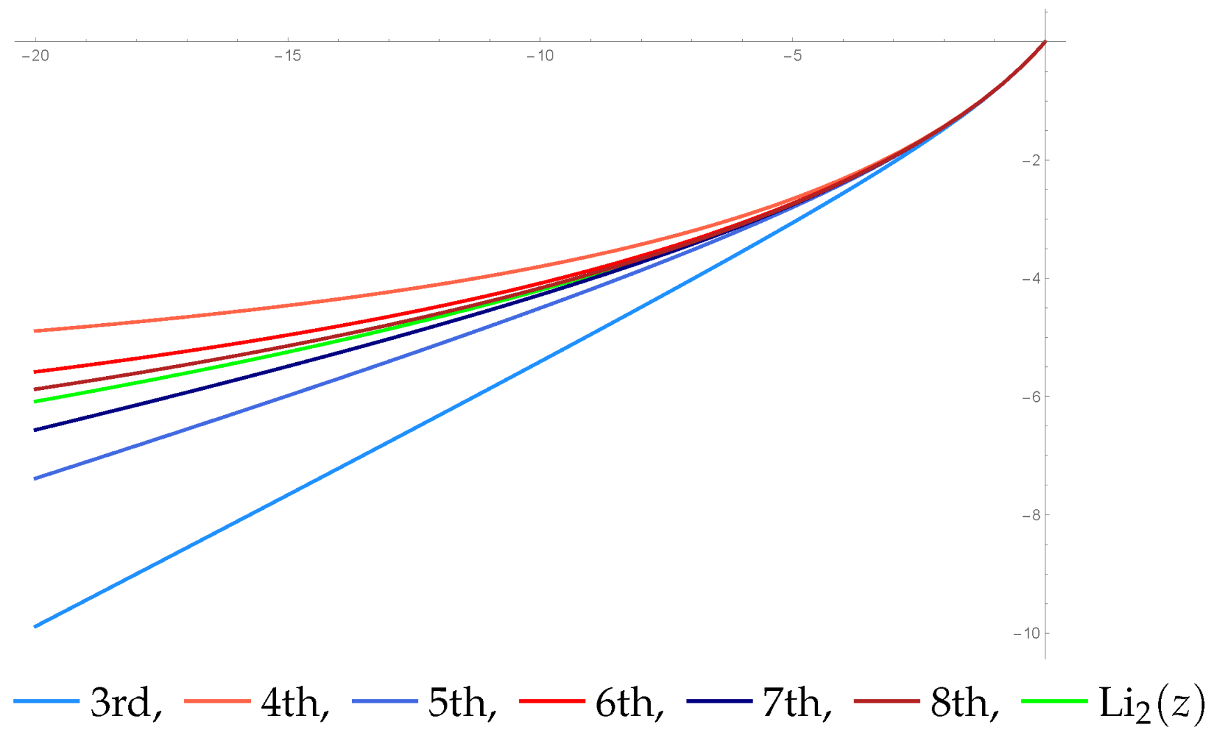
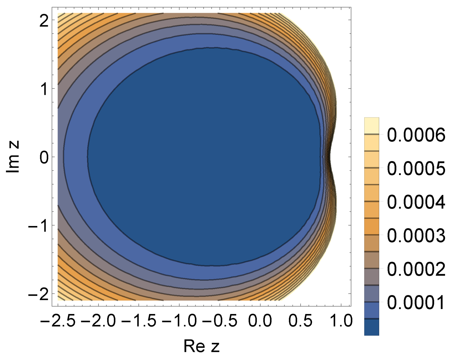
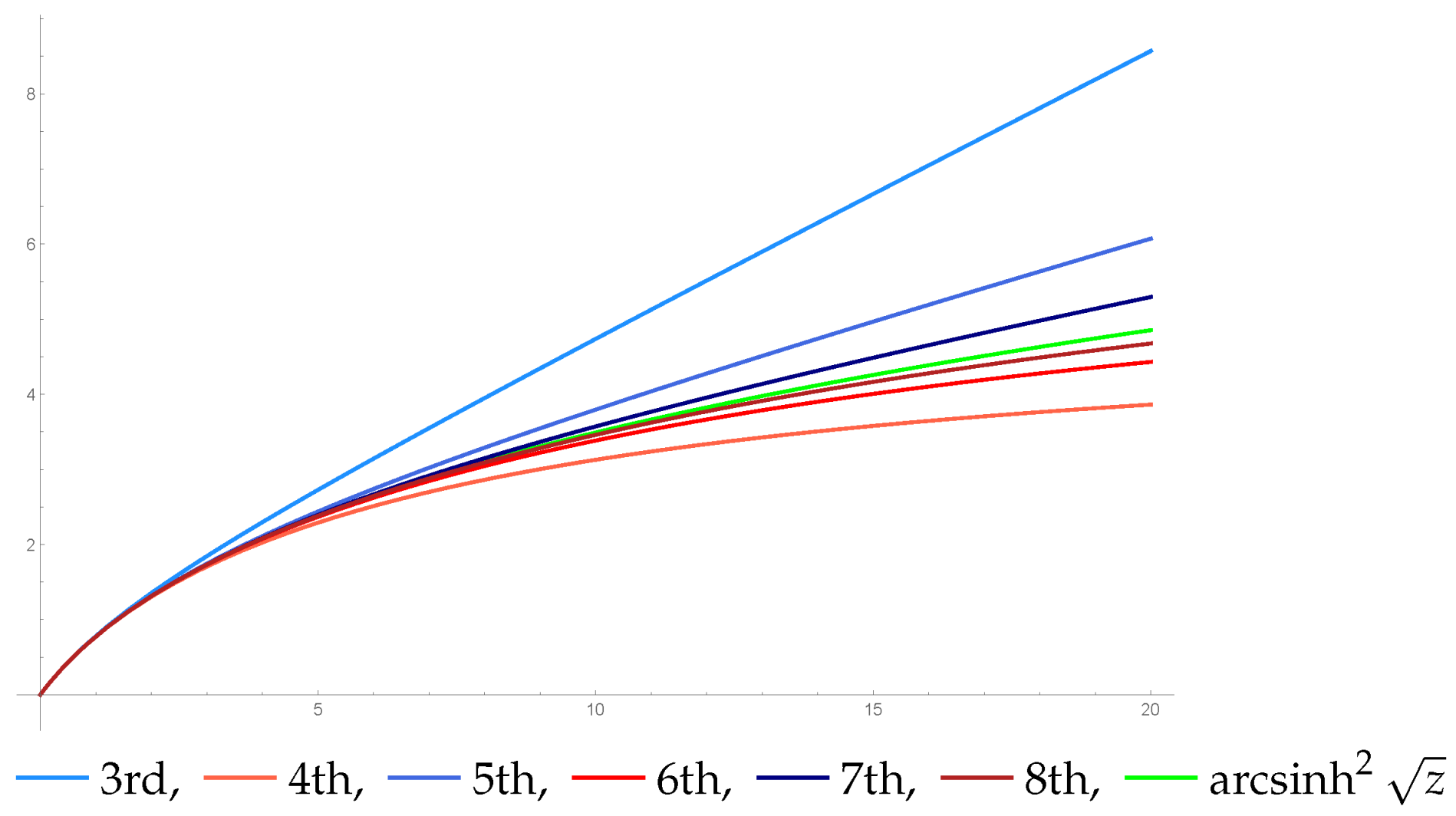
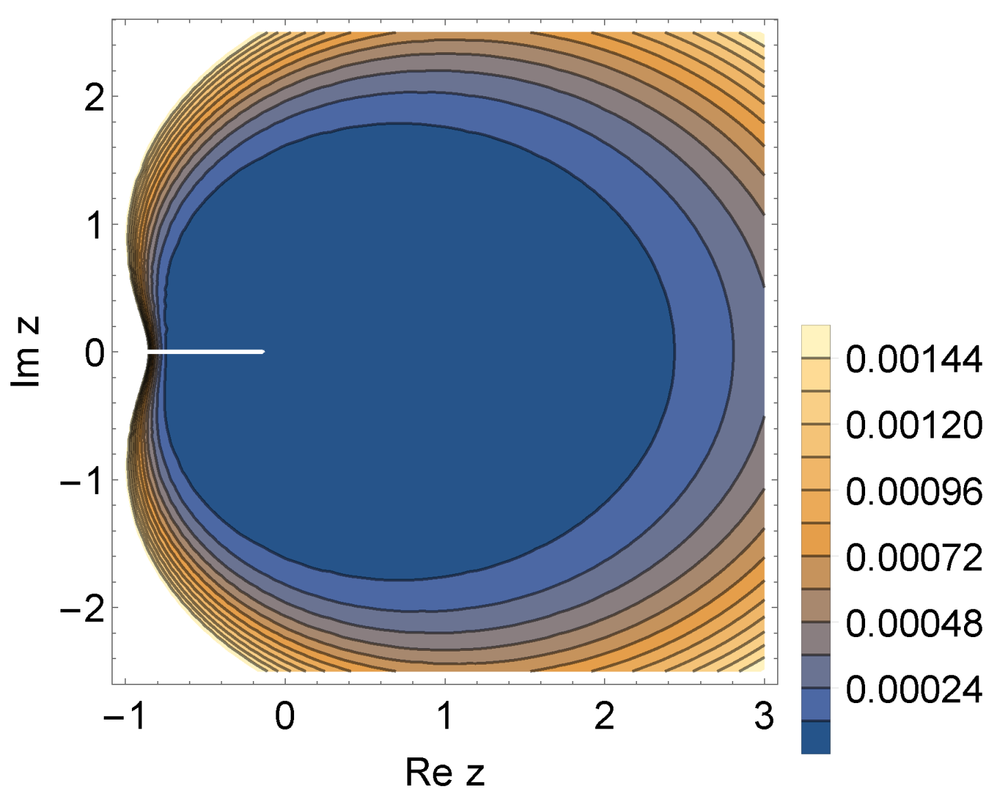
3. Numerical Experiments

In this section, we illustrate the use of branched continued fractions to approximate the solutions of differential equations. Approximation of some analytic functions by branched continued fractions can be found in [42,52,53,54].

It should be noted that if the conditions of Corollary 1 are satisfied, then the branched continued fraction (45) satisfies the differential Equation (2) in which $a_1=1.$ This means that the approximations of (45) can be used to approximate the solution of this differential equation in the region (37).

For example, we set $a_2=1/2,$$a_3=1,$$b_1=6,$$b_2=2.$ Then, it is obvious that the parameters satisfy the conditions (44) and, therefore, from (15)–(20), where $a_1=0$ and $b_1$ replaced by $b_1-1,$ we have such approximations

$$f_1^{1,1}\left(z\right)=1,f_2^{1,1}\left(z\right)=\frac{28}{28-z},f_3^{1,1}\left(z\right)=\frac{168-11z}{168-18z},etc.,$$

for the solution $u\left(z\right)$ of differential equation

$$z^3(1-z)\frac{d^{3}u}{d{z}^3}+z\left(\frac{z}{2}-2\right)\frac{d^{2}u}{d{z}^2}+(z-6)\frac{du}{dz}+u=0.$$

(46)

The values of these approximations are given in

Table 1. Approximation of the solution of differential Equation (46) by the branched continued fraction (45) and the generalized hypergeometric series ${}_3{F}_2(1,1/2,1;6,2;z)$.

n	${\mathit{f}}_{\mathit{n}}^{1,1}\left(0.1\right)$	${\mathit{S}}_{\mathit{n}}\left(0.1\right)$	${\mathit{f}}_{\mathit{n}}^{1,1}(-1.0)$	${\mathit{S}}_{\mathit{n}}(-1.0)$	${\mathit{f}}_{\mathit{n}}^{1,1}(-4.0)$	${\mathit{S}}_{\mathit{n}}(-4.0)$
1	1.000000000000	1.000000000000	1.000000000000	1.000000000000	1.000000000000	1.000000000000
2	1.004184100418	1.004166666667	0.960000000000	0.958333333333	0.857142857143	0.833333333333
3	1.004227053140	1.004226190476	0.963541666667	0.964285714290	0.893939393940	0.928571428570
4	1.004227621300	1.004227585565	0.963169003257	0.962890625000	0.883767535070	0.839285714286
5	1.004227630503	1.004227628968	0.963214851933	0.963324652778	0.886929122814	0.950396825397
6	1.004227630666	1.004227630596	0.963208892004	0.963161892361	0.885923553202	0.783730158730
7	1.004227630669	1.004227630666	0.963209728694	0.963231646825	0.886262535450	1.069444444444
8	1.004227630669	1.004227630669	0.963209609365	0.963198586116	0.886148086455	0.527777777778
9	1.004227630669	1.004227630669	0.963209627248	0.963215540326	0.886188283668	1.638888888889
10	1.004227630669	1.004227630669	0.963209624564	0.963206276061	0.886174256708	−0.789682539683
11	1.004227630669	1.004227630669	0.963209624981	0.963211610032	0.886179300167	4.803391053391
12	1.004227630669	1.004227630669	0.963209624917	0.963208401315	0.886177503402	−8.654942279943
13	1.004227630669	1.004227630669	0.963209624927	0.963210404948	0.886178158992	24.960442335442

together with the values of the partial sums $S_n\left(z\right)$ of ${}_3{F}_2(1,1/2,1;6,2;z)$ for $1\le n\le 13$ and for the various value of $z.$ Those numbers illustrate the rate of convergence of $f_n^{1,1}\left(z\right)$ and $S_n\left(z\right)$ to $u\left(z\right)$ as n increases. Comparing them, we see that the branched continued fraction (45) gives better approximations of the solution of differential Equation (46) than the generalized hypergeometric series ${}_3{F}_2(1,1/2,1;6,2;z).$

It should be noted that analogous results can be observed in cases (a)–(c) given at the end of Section 2.3.

Finally, we consider the approximation of functions by constructed expansions.

The dilogarithm is the function defined by the power series (see, for example, [55])

$${Li}_2\left(z\right)=\sum _{k=1}^{\infty }\frac{z^k}{k^2}\mathrm{for}\left|z\right|<1$$

with an analytic continuation given by

$${Li}_2\left(z\right)=-{\int }_0^z\frac{ln(1-u)}{u}du\mathrm{for}z\in \mathbb{C}\backslash [1,+\infty ).$$

(47)

In [56], it is shown that

$${Li}_2\left(z\right)=\frac{z}{1}\genfrac{}{}{0pt}{}{}{+}\frac{a_{2}z}{1}\genfrac{}{}{0pt}{}{}{+}\frac{a_{3}z}{1}\genfrac{}{}{0pt}{}{}{+}\dots \mathrm{for}z\in \mathbb{C}\backslash [1,+\infty ),$$

(48)

where

$$a_{2n}=\frac{A_n^{\left(1\right)}{A}_{n-1}^{\left(0\right)}}{A_n^{\left(0\right)}{A}_{n-1}^{\left(1\right)}},a_{2n+1}=\frac{A_{n-1}^{\left(1\right)}{A}_{n+1}^{\left(0\right)}}{A_n^{\left(0\right)}{A}_n^{\left(1\right)}},A_n^{\left(r\right)}=det{∥\frac{{(-1)}^{i+j+r}}{{(r+i+j-1)}^2}∥}_{1\le i,j\le n}.$$

In addition, ${Li}_2\left(z\right)$ can be expressed as (see, ([57], Section 2.6))

$${Li}_2\left(z\right)=z{}_3{F}_2(1,1,1;2,2;z).$$

(49)

It follows from Corollary 1 that in the region (37) the function ${Li}_2\left(z\right)$ is represented by a branched continued fraction of the form

$${\displaystyle \frac{z}{1-{\displaystyle \frac{c_{2,1}^{1,1}z}{1-{\displaystyle \frac{c_{2,1,1,1}^{1,1}z}{1-{\displaystyle \frac{c_{2,1,1,1,2,1}^{1,1}z}{1-{}_{\ddots }}}}}-{\displaystyle \frac{c_{2,1,2,2}^{1,1}z}{1-{\displaystyle \frac{c_{2,1,2,2,1,2}^{1,1}z}{1-{}_{\ddots }}}-{\displaystyle \frac{c_{2,1,2,2,2,1}^{1,1}z}{1-{}_{\ddots }}}}}}}}},$$

(50)

where $c_{{\left(ij\right)}_k}^{1,1},$${\left(ij\right)}_k\in {\mathcal{I}}_{1,1},$ defined by formulas (15)–(20), where $a_1=0$ and $b_1$ replaced by $b_1-1.$

Plots of the values of the nth approximants of the branched continued fraction (50) are shown in Figure 1. Here we can see the so-called `fork property’ for a branched continued fraction with positive elements (see [18] (p. 29)). That is, the plots of the values of even (odd) approximations of (50) approaches from above (below) to the plot of the function ${Li}_2\left(z\right).$

Figure 2 shows the plots where the approximant $f_8^{1,1}\left(z\right)$ of the branched continued fraction (50) guarantees certain truncation error bounds for function ${Li}_2\left(z\right)$.

The numerical illustration of (48)–(50) is given in the

Table 2. Relative error of 5th partial sum and 5th approximants for ${Li}_2\left(z\right)$.

z	(47)	(49)	(48)	(50)
$0.2$	$0.2110037754$	$9.88869\times {10}^{-6}$	$3.84790\times {10}^{-7}$	$3.79061\times {10}^{-7}$
$0.1$	$0.1026177911$	$2.92233\times {10}^{-7}$	$9.50960\times {10}^{-9}$	$9.36538\times {10}^{-9}$
$-0.2$	$-0.1908001378$	$8.12951\times {10}^{-6}$	$1.64637\times {10}^{-7}$	$1.62051\times {10}^{-7}$
$-0.4$	$-0.3658325775$	$2.40912\times {10}^{-4}$	$3.70070\times {10}^{-6}$	$3.64181\times {10}^{-6}$
$-0.5$	$-0.4484142069$	$7.10129\times {10}^{-4}$	$9.59022\times {10}^{-6}$	$9.43694\times {10}^{-6}$
$-0.7$	$-0.6051584023$	$3.58461\times {10}^{-3}$	$3.80158\times {10}^{-5}$	$3.74047\times {10}^{-5}$
$-0.9$	$-0.7521631792$	$1.18992\times {10}^{-2}$	$1.00919\times {10}^{-4}$	$9.92914\times {10}^{-5}$
$-5$	$-2.749279126$	$3.48554\times {10}^{+1}$	$1.83416\times {10}^{-2}$	$1.80702\times {10}^{-2}$
$-25$	$-6.785907900$	$5.42019\times {10}^{+4}$	$2.91475\times {10}^{-1}$	$2.88304\times {10}^{-1}$

. Here we compare the relative errors of the approximation of function (47) by the partial sums of the power series and the approximants of the continued fraction and the branched continued fraction. As a results, the nth approximant of (50) is eventually a better approximation to (47) than the nth partial sum of (49) and the nth approximant of (48) is.

In [58], it is given that function

$${arcsinh}^2\sqrt{z}={ln}^2(\sqrt{z}+\sqrt{z+1})$$

(51)

(here the principal branch of the square root is assumed) has a generalized hypergeometric series in the form

$$z{}_3{F}_2(1,1,1;3/2,2;-z)=\sum _{n=0}^{\infty }\frac{{(-1)}^n{\left({\left(1\right)}_n\right)}^3}{{(3/2)}_n{\left(2\right)}_n}\frac{z^{n+1}}{n!}.$$

(52)

So, it follows from Corollary 1 that the branched continued fraction

$${\displaystyle \frac{z}{1+{\displaystyle \frac{z/3}{1+{\displaystyle \frac{z/15}{1+{\displaystyle \frac{2z/15}{1+{}_{\ddots }}}}}+{\displaystyle \frac{8z/21}{1+{\displaystyle \frac{4z/75}{1+{}_{\ddots }}}+{\displaystyle \frac{3z/7}{1+{}_{\ddots }}}}}}}}}$$

(53)

is an analytic continuation of function (51) in the region

$$H_{\epsilon }=\{z\in \mathbb{C}:|arg\left(z\right)|\le \pi /(1+\epsilon )\},0<\epsilon <1.$$

Plots of the values of the nth approximants of the branched continued fraction (53) for ${arcsinh}^2\sqrt{z}$ are shown in Figure 3.

Figure 4 shows the plots where the approximant $f_8^{1,1}\left(z\right)$ of the branched continued fraction (53) guarantees certain truncation error bounds for function ${arcsinh}^2\sqrt{z}.$

Finally, a numerical illustration of (52) and (53) is given in the

Table 3. Relative error of 5th partial sum and 5th approximant for ${arcsinh}^2\sqrt{z}$.

z	(51)	(52)	(53)
$0.1$	0.09683377	$5.89297\times {10}^{-7}$	$9.38113\times {10}^{-9}$
$0.2$	0.18792863	$1.81135\times {10}^{-5}$	$2.44604\times {10}^{-7}$
$0.4$	0.35575900	$5.39204\times {10}^{-4}$	$5.37787\times {10}^{-6}$
$0.7$	0.57918140	$8.01911\times {10}^{-3}$	$5.37870\times {10}^{-5}$
$0.9$	0.71337919	$2.62446\times {10}^{-2}$	$1.40695\times {10}^{-4}$
1	0.77681940	$4.26521\times {10}^{-2}$	$2.07391\times {10}^{-4}$
3	1.73437810	$8.86578\times {10}^{-1}$	$6.54173\times {10}^{-3}$
10	3.49148329	$9.99511\times {10}^{-1}$	$8.03203\times {10}^{-2}$
50	7.04436144	$9.99999\times {10}^{-1}$	$4.29712\times {10}^{-1}$

.

Here we have results like to the results in the previous example.

4. Discussion

In [26], the authors constructed branched continued fraction expansions for some ratios of the generalized hypergeometric function ${}_3{F}_2.$ In this work, we have constructed new expansions and investigated their convergence in some region together with the already known ones. This allows us to approximate the solutions of certain differential equations and also analytic functions, represented by generalized hypergeometric function ${}_3{F}_2,$ using branched continued fractions. The result is a generalization of the classical continued fraction expansions of Gauss’s hypergeometric function ratios.

Compared with power series or multiple power series under certain conditions, branched continued fractions have wider convergence regions and are endowed with the property of numerical stability. This makes them an effective tool for rational approximation in the theory approximation. Studying the branched continued fractions is to develop new and effective methods for establishing convergence criteria and finding estimates of the rate of convergence.

Despite the fact that the established convergence region for the constructed expansions is wider than the convergence region of the corresponding generalized hypergeometric function ${}_3{F}_2,$ the problem of studying wider convergence regions and establishing estimates of the of convergence rate of the expansions mentioned above still remains open.

The proposed methods for constructing and studying the branched continued fraction expansions of the ratios of generalized hypergeometric function ${}_3{F}_2$ can also be applied to construct the expansions of other relations of generalizations of the Gauss hypergeometric function. This, in turn, will allow the use of branched continued fractions to approximate the solutions of some differential equations and their system, which can be used in applied problems in physics, astronomy, economics, etc. Here it is appropriate to mention one of the interesting applications of continued fractions in modelling the birth-death processes in the works [59,60,61]. Finally, we point to the works [62,63,64], where is no less interesting application of continued and branched continued fractions in chemical graph theory.

References

1. Abd-Rabo, M.A.; Zakarya, M.; Cesarano, C.; Aly, S. Bifurcation analysis of time-delay model of consumer with the advertising effect. Symmetry 2021, 13, 417. [Google Scholar] [CrossRef]
2. AlNemer, G.; Kenawy, M.; Zakarya, M.; Cesarano, C.; Rezk, H.M. Generalizations of Hardy’s type inequalities via conformable calculus. Symmetry 2021, 13, 242. [Google Scholar] [CrossRef]
3. Duan, S.; Song, W.; Zio, E.; Cattani, C.; Li, M. Product technical life prediction based on multi-modes and fractional Levy stable motion. Mech. Syst. Signal Process. 2021, 161, 107984. [Google Scholar] [CrossRef]
4. Elayaraja, R.; Ganesan, V.; Bazighifan, O.; Cesarano, C. Oscillation and asymptotic properties of differential equations of third-order. Axioms 2021, 10, 192. [Google Scholar] [CrossRef]
5. Mohammad, M.; Trounev, A.; Cattani, C. The dynamics of COVID-19 in the UAE based on fractional derivative modeling using Riesz wavelets simulation. Adv. Differ. Equ. 2021, 2021, 115. [Google Scholar] [CrossRef]
6. Wojtowicz, M.; Bodnar, D.; Shevchuk, R.; Bodnar, O.; Bilanyk, I. The Monte Carlo type method of attack on the RSA cryptosystem. In Proceedings of the 10th International Conference on Advanced Computer Information Technologies, Institute of Applied Informatics of Deggendorf Institute of Technology, Deggendorf, Germany, 13–15 May 2020; Institute of Electrical and Electronics Engineers Inc.: Deggendorf, Germany, 2020; pp. 755–758. [Google Scholar]
7. Baranetskij, Y.O.; Demkiv, I.I.; Kopach, M.I.; Solomko, A.V. Interpolational (L,M)-rational integral fraction on a continual set of nodes. Carpathian Math. Publ. 2021, 13, 587–591. [Google Scholar]
8. Cuyt, A.A.M.; Petersen, V.; Verdonk, B.; Waadeland, H.; Jones, W.B. Handbook of Continued Fractions for Special Functions; Springer: Dordrecht, The Netherlands, 2008. [Google Scholar]
9. Lascu, D.; Sebe, G.I. A Gauss–Kuzmin–Lévy theorem for Rényi-type continued fractions. Acta Arith. 2020, 193, 283–292. [Google Scholar] [CrossRef]
10. Lascu, D.; Sebe, G.I. A Lochs-type approach via entropy in comparing the efficiency of different continued fraction algorithms. Mathematics 2021, 9, 255. [Google Scholar] [CrossRef]
11. Lima, H.; Loureiro, A. Multiple orthogonal polynomials associated with confluent hypergeometric functions. J. Approx. Theory 2020, 260, 105484. [Google Scholar] [CrossRef]
12. Jones, W.B.; Thron, W.J. Continued Fractions: Analytic Theory and Applications; Addison-Wesley Pub. Co.: Reading, MA, USA, 1980. [Google Scholar]
13. Khrushchev, S. Orthogonal Polynomials and Continued Fractions; Cambridge University Press: New York, NY, USA, 2008. [Google Scholar]
14. Lorentzen, L.; Waadeland, H. Continued Fractions—Volume 1: Convergence Theory, 2nd ed.; Atlantis Press: Amsterdam, The Netherlands, 2008. [Google Scholar]
15. Sebe, G.I.; Lascu, D. Convergence rate for Rényi-type continued fraction expansions. Period. Math. Hung. 2020, 81, 239–249. [Google Scholar] [CrossRef] [Green Version]
16. Wall, H.S. Analytic Theory of Continued Fractions; D. Van Nostrand Co.: New York, NY, USA, 1948. [Google Scholar]
17. Zou, L.; Song, L.; Wang, X.; Chen, Y.; Zhang, C.; Tang, C. Bivariate Thiele-like rational interpolation continued fractions with parameters based on virtual points. Mathematics 2020, 8, 71. [Google Scholar] [CrossRef] [Green Version]
18. Bodnar, D.I. Branched Continued Fractions; Naukova Dumka: Kyiv, Ukraine, 1986. (In Russian) [Google Scholar]
19. Bodnar, D.I.; Zators’kyi, R.A. Generalization of continued fractions. I. J. Math. Sci. 2012, 183, 54–64. [Google Scholar] [CrossRef]
20. Bodnar, D.I.; Zators’kyi, R.A. Generalization of continued fractions. II. J. Math. Sci. 2012, 184, 45–55. [Google Scholar] [CrossRef]
21. Bodnarchuk, P.I.; Skorobogatko, V.Y. Branched Continued Fractions and Their Applications; Naukova Dumka: Kyiv, Ukraine, 1974. (In Ukrainian) [Google Scholar]
22. Cuyt, A. A review of multivariate Padé approximation theory. J. Comput. Appl. Math. 1985, 12–13, 221–232. [Google Scholar] [CrossRef] [Green Version]
23. Cuyt, A.; Verdonk, B. A review of branched continued fraction theory for the construction of multivariate rational approximants. Appl. Numer. Math. 1988, 4, 263–271. [Google Scholar] [CrossRef]
24. Murphy, J.A.; O’Donohoe, M.R. A two-variable generalization of the Stieltjes-type continued fraction. J. Comput. Appl. Math. 1978, 4, 181–190. [Google Scholar] [CrossRef] [Green Version]
25. Petreolle, M.; Sokal, A.D. Lattice paths and branched continued fractions II. Multivariate Lah polynomials and Lah symmetric functions. Eur. J. Combin. 2021, 92, 103235. [Google Scholar] [CrossRef]
26. Petreolle, M.; Sokal, A.D.; Zhu, B.X. Lattice paths and branched continued fractions: An infinite sequence of generalizations of the Stieltjes-Rogers and Thron-Rogers polynomials, with coefficientwise Hankel-total positivity. arXiv 2020, arXiv:1807.03271v2. [Google Scholar]
27. Siemaszko, W. Branched continued fractions for double power series. J. Comput. Appl. Math. 1980, 6, 121–125. [Google Scholar] [CrossRef] [Green Version]
28. Skorobogatko, V.Y. Theory of Branched Continued Fractions and Its Applications in Computational Mathematics; Nauka: Moscow, Russia, 1983. (In Russian) [Google Scholar]
29. Gauss, C.F. Disquisitiones generales circa seriem infinitam 1 + α β 1 · γ x + α ( α + 1 ) β ( β + 1 ) 1 · 2 · ( γ + 1 ) x x + α ( α + 1 ) ( α + 2 ) β ( β + 1 ) ( β + 2 ) 1 · 2 · 3 · γ ( γ + 1 ) ( γ + 3 ) x 3 + etc. In Commentationes Societatis Regiae Scientiarum Gottingensis Recentiores; Classis Mathematicae, 1812; H. Dieterich: Gottingae, Germany, 1813; Volume 2, pp. 3–46. [Google Scholar]
30. Bodnar, D.I. Expansion of a ratio of hypergeometric functions of two variables in branching continued fractions. J. Math. Sci. 1993, 64, 1155–1158. [Google Scholar] [CrossRef]
31. Bodnar, D.I.; Manzii, O.S. Expansion of the ratio of Appel hypergeometric functions F3 into a branching continued fraction and its limit behavior. J. Math. Sci. 2001, 107, 3550–3554. [Google Scholar] [CrossRef]
32. Bodnar, D.I. Multidimensional C-Fractions. J. Math. Sci. 1998, 90, 2352–2359. [Google Scholar] [CrossRef]
33. Bodnar, D.I.; Hoyenko, N.P. Approximation of the ratio of Lauricella functions by a branched continued fraction. Mat. Studii 2003, 20, 210–214. [Google Scholar]
34. Hoyenko, N.; Hladun, V.; Manzij, O. On the infinite remains of the Nórlund branched continued fraction for Appell hypergeometric functions. Carpathian Math. Publ. 2014, 6, 11–25. (In Ukrainian) [Google Scholar] [CrossRef] [Green Version]
35. Hoyenko, N.; Antonova, T.; Rakintsev, S. Approximation for ratios of Lauricella–Saran fuctions FS with real parameters by a branched continued fractions. Math. Bul. Shevchenko Sci. Soc. 2011, 8, 28–42. (In Ukrainian) [Google Scholar]
36. Antonova, T.; Dmytryshyn, R.; Kravtsiv, V. Branched continued fraction expansions of Horn’s hypergeometric function H3 ratios. Mathematics 2021, 9, 148. [Google Scholar] [CrossRef]
37. Bailey, W.N. Generalised Hypergeometric Series; Cambridge University Press: Cambridge, UK, 1935. [Google Scholar]
38. Herschel, J.F.W. A Collection of Examples of the Applications of the Calculus of Finite Differences; Printed by J. Smith and sold by J. Deighton & Sons: Cambridge, UK, 1820. [Google Scholar]
39. Antonova, T.M. On convergence criteria for branched continued fraction. Carpathian Math. Publ. 2020, 12, 157–164. [Google Scholar] [CrossRef]
40. Bodnar, D.I.; Bilanyk, I.B. On the convergence of branched continued fractions of a special form in angular domains. J. Math. Sci. 2020, 246, 188–200. [Google Scholar] [CrossRef]
41. Bodnar, D.I.; Bilanyk, I.B. Parabolic convergence regions of branched continued fractions of the special form. Carpathian Math. Publ. 2021, 13, 619–630. [Google Scholar]
42. Bodnar, D.I.; Dmytryshyn, R.I. Multidimensional associated fractions with independent variables and multiple power series. Ukr. Math. J. 2019, 71, 370–386. [Google Scholar] [CrossRef]
43. Bilanyk, I.B.; Bodnar, D.I.; Buyak, L.M. Representation of a quotient of solutions of a four-term linear recurrence relation in the form of a branched continued fraction. Carpathian Math. Publ. 2019, 11, 33–41. [Google Scholar] [CrossRef]
44. Dmytryshyn, R.I. Convergence of multidimensional A- and J-fractions with independent variables. Comput. Methods Funct. Theory 2021. [Google Scholar] [CrossRef]
45. Dmytryshyn, R.I. On some of convergence domains of multidimensional S-fractions with independent variables. Carpathian Math. Publ. 2019, 11, 54–58. [Google Scholar] [CrossRef]
46. Antonova, T.M.; Dmytryshyn, R.I. Truncation error bounds for branched continued fraction i 1 = 1 N a i ( 1 ) 1 + i 2 = 1 i 1 a i ( 2 ) 1 + i 3 = 1 i 2 a i ( 3 ) 1 + . Ukr. Math. J. 2020, 72, 1018–1029. [Google Scholar] [CrossRef]
47. Antonova, T.M.; Dmytryshyn, R.I. Truncation error bounds for branched continued fraction whose partial denominators are equal to unity. Mat. Stud. 2020, 54, 3–14. [Google Scholar]
48. Bodnar, O.S.; Dmytryshyn, R.I.; Sharyn, S.V. On the convergence of multidimensional S-fractions with independent variables. Carpathian Math. Publ. 2020, 12, 353–359. [Google Scholar] [CrossRef]
49. Bodnar, D.I.; Bilanyk, I.B. Estimates of the rate of pointwise and uniform convergence for branched continued fractions with nonequivalent variables. Mat. Method. Fiz. Mech. Polya 2019, 6, 72–82. (In Ukrainian) [Google Scholar]
50. Bilanyk, I.B. A truncation error bound for some branched continued fractions of the special form. Mat. Stud. 2019, 52, 115–123. [Google Scholar] [CrossRef]
51. Antonova, T.M. Multidimensional generalization of the theorem on parabolic domains of convergence of continued fractions. Mat. Met. Fiz.-Mekh. Polya. 1999, 42, 7–12. (In Ukrainian) [Google Scholar]
52. Dmytryshyn, R.I. On the expansion of some functions in a two-dimensional g-fraction independent variables. J. Math. Sci. 2012, 181, 320–327. [Google Scholar] [CrossRef]
53. Dmytryshyn, R.I.; Sharyn, S.V. Approximation of functions of several variables by multidimensional S-fractions with independent variables. Carpathian Math. Publ. 2021, 13, 592–607. [Google Scholar]
54. Dmytryshyn, R.I. Two-dimensional generalization of the Rutishauser qd-algorithm. J. Math. Sci. 2015, 208, 301–309. [Google Scholar] [CrossRef]
55. Zagier, D. The dilogarithm function. In Frontiers in Number Theory, Physics, and Geometry II; Cartier, P., Moussa, P., Julia, B., Vanhove, P., Eds.; Springer: Berlin, Germany, 2007; pp. 3–65. [Google Scholar]
56. Cvijović, D.; Klinowsky, J. Continued-fraction expansions for the Riemann zeta function and polylogarithms. Proc. Amer. Math. Soc. 1997, 125, 2543–2550. [Google Scholar] [CrossRef]
57. Andrews, G.E.; Askey, R.; Roy, R. Special Functions; Cambridge University Press: Cambridge, UK, 1999. [Google Scholar]
58. Krupnikov, E.D.; Kölbig, K.S. Some special cases of the generalized hypergeometric function q+lFq. J. Comput. Appl. Math. 1997, 78, 75–95. [Google Scholar] [CrossRef] [Green Version]
59. Ho, L.S.T.; Xu, J.; Crawford, F.W.; Minin, V.N.; Suchard, M.A. Birth/birth-death processes and their computable transition probabilities with biological applications. J. Math. Biol. 2018, 76, 911–944. [Google Scholar] [CrossRef]
60. Jones, W.B.; Magnus, A. Application of Stieltjes fractions to birth-death processes. In Padé and Rational Approximation; Saff, E.B., Varga, R.S., Eds.; Academic Press: New York, NY, USA, 1977; pp. 173–179. [Google Scholar]
61. Murphy, J.A.; O’Donohoe, M.R. Some properties of continued fractions with applications in Markov processes. J. Inst.Math. Appl. 1975, 16, 57–71. [Google Scholar] [CrossRef]
62. Komatsu, T. Asymmetric circular graph with Hosoya index and negative continued fractions. Carpathian Math. Publ. 2021, 13, 608–618. [Google Scholar]
63. Komatsu, T. Branched continued fractions associated with Hosoya index of the tree graph. MATCH Commun. Math. Comput. Chem. 2020, 84, 399–428. [Google Scholar]
64. Komatsu, T. Continued fraction expansions of the generating functions of Bernoulli and related numbers. Indag. Math. 2020, 31, 695–713. [Google Scholar] [CrossRef]
Figure 1. The plots of values of the nth approximants of (50) for Li 2 ( z ) .
Axioms 10 00310 g001
Figure 2. The plots where the approximant f 8 1 , 1 ( z ) of (50) guarantees certain truncation error bounds for Li 2 ( z ) .
Axioms 10 00310 g002
Figure 3. The plots of values of the nth approximants of (53) for arcsinh 2 z .
Axioms 10 00310 g003
Figure 4. The plots where the approximant f 8 1 , 1 ( z ) of (53) guarantees certain truncation error bounds for arcsinh 2 z .
Axioms 10 00310 g004