Hybrid Method for Simulation of a Fractional COVID-19 Model with Real Case Application

Abstract

In this research, we provide a mathematical analysis for the novel coronavirus responsible for COVID-19, which continues to be a big source of threat for humanity. Our fractional-order analysis is carried out using a non-singular kernel type operator known as the Atangana-Baleanu-Caputo (ABC) derivative. We parametrize the model adopting available information of the disease from Pakistan in the period 9 April to 2 June 2020. We obtain the required solution with the help of a hybrid method, which is a combination of the decomposition method and the Laplace transform. Furthermore, a sensitivity analysis is carried out to evaluate the parameters that are more sensitive to the basic reproduction number of the model. Our results are compared with the real data of Pakistan and numerical plots are presented at various fractional orders.

1. Introduction

The novel coronavirus SARS-CoV-2, responsible for COVID-19, which is member of the family of Severe Acute Respiratory Syndrome (SARS) viruses, has been recognized as the most dangerous virus of this decade [1]. This virus has become the new novel strain of the SARS family, which was not recognized in humans before [2]. COVID-19 has not just affected humans, but also a number of animals have been infected by the virus. The SARS-CoV-2 virus has been transmitted from human to human and similarly in animals, but its origin is still a controversy [3]. Infected humans and different species of various animals are recognized as active causes of spreading of the virus [1]. In the past, some similar viruses, like the Middle East Respiratory Syndrome Coronavirus (MERS-CoV), were spread out from camels to human population, and for SARS-CoV-1 the civet was recognized as the source of spreading into humans. For COVID-19, the main source or the major reason of spreading is human-to-human interaction, where the virus transmission is easily made by an infected person to a susceptible one. Currently, thousands of research studies have been proposed and many predictions have been given on COVID-19 dynamics, see in [4,5,6,7,8] and references therein. Our paper is, however, different from those in the literature. In [4], special focus is given to the transmissibility of the so-called superspreaders, with numerical simulations being given for data of Galicia, Spain, and Portugal. It turns out that, for each region, the order of the Caputo derivative takes a different value, always different from one, showing the relevance of considering fractional-order models to investigate COVID-19. The work in [5] studies the COVID-19 pandemic in Portugal until the end of the three states of emergency, describing well what has happen in Portugal with respect to the evolution of active infected and hospitalized individuals. In [6,7], a non-fractional but stochastic time-delayed model for COVID-19 is given, with the aim to study the situation of Morocco. In [8], the authors provide a S-E-I-P-A-H-R-F model while here we propose a much simpler P-I-Q model (our model has only three state variables while the model in [8] is much more complex, with eight state variables). In [8], the authors use the classical operator of Caputo; differently, here we use the more recent ABC derivatives that, in contrast, use non-singular kernels that allow us to consider a much simpler model. While the main result in [8] is the proof of the global stability of the disease free equilibrium; in contrast, here we prove Ulam–Hyers stability. We also construct a practical algorithm to compute numerically the solution of the model (see Section 5), while such algorithmic approach is not addressed in [8]. Moreover, we do a sensitivity analysis to the parameters of the model. Such sensitivity analysis is also not addressed in [8]. In contrast with the work in [8], that investigates the realities of Wuhan, Spain, and Portugal, we study the case of Pakistan.

COVID-19 generally transfers by interaction with humans in close contact for a particular time period, with most common symptoms of sneezing and coughing. The virus droplets stay on the layer of matters and when they come to the contact with any susceptible human, then the virus symptoms easily transfer to the individuals. Such infected humans can pass the infection to others by touching their mouth, eyes, or nose. This virus has the strength to be alive on different surfaces, like cardboard and copper, for many hours up to some days. As the time passes, the amount of the virus symptoms decreases over a time span and might not be alive in sufficient amount for spreading the infection. It has been recorded that the symptoms appearance and COVID-19 infection initial stage lies between 1 to 14 days [1]. Several countries have prepared and implemented a COVID-19 vaccine program and are trying to protect their populations. However, to date, there is yet no treatment available. At present, the most effect way to protect ourselves from the virus remains the quarantine or isolation, effective use of mask, following the guidelines that have been passed by governments of all countries along with the World Health Organization (WHO).

Modeling of infectious diseases has a rich literature and a number of research articles have been developed, both using classical dynamical systems as well as fractional models [4,8]. Fractional-order derivatives can be useful and helpful as compared to classical derivatives, because the dynamics of real phenomena can be comprehensively understood by fractional-order derivatives due to its special properties, i.e., hereditary and memory [9,10,11,12,13,14,15,16]. For a comparison between classical (integer-order) and fractional-order models, see in [4,8]. Roughly speaking, ordinary derivatives cannot distinguish the phenomenon at two distinct closed points. To sort out this problem of ordinary derivatives, generalized derivatives have been introduced in the framework of fractional calculus [17]. The first concept of fractional-order derivative was given by Leibniz and L’Hôpital in 1695. Aiming quantitative analysis, optimization, and numerical estimations, many number of attempts have been made by employing fractional differential equations (FDEs) [1,2,18,19,20,21,22,23,24,25,26,27,28,29,30,31,32,33,34,35,36,37,38]. The growing interest in the modeling of complex real-world issues with the use of FDEs is due to its numerous properties that can not be found in the ordinary sense. These characteristics allow FDEs to model effectively not only non-Markovian processes but also non-Gaussian phenomena [39]. Different non-classical fractional-order derivatives and different kinds of FDEs were proposed [40,41,42]. Among them, one has the Atangana-Baleanu-Caputo (ABC) derivative, which is a nonlocal fractional derivative with a non-singular kernel, connected with various applications. For a discussion of the ABC and related operators see in [43,44], and for their use on contemporary modeling we refer the interested reader to the works in [45,46,47,48].

The famous method of decomposition was developed from the 1970s to the 1990s by George Adomian, to analytically handle nonlinear problems. After that, the Adomian decomposition method became a powerful tool to simulate analytical or approximate solutions for various problems of an applied nature. Many mathematical models have been studied by the applications of homotopy, Laplace Adomian Decomposition Method (LADM), and variational methods [49,50,51]. To the best of our knowledge, no one has studied a variable order epidemic model with ABC derivatives by the LADM. Motivated by this fact, here we study a fractional-order COVID-19 epidemic model with ABC derivatives by the Laplace Adomian decomposition algorithm. In particular, we use Banach and Krassnoselskii fixed point theorems to define some sufficient conditions to prove existence and uniqueness of solution. As stability is important for the estimated solution, we consider Ulam type stability through nonlinear functional analysis. The aforementioned stability is investigated for ordinary fractional derivatives in many research papers, see, e.g., in [52,53,54], but research on Ulam type stability regarding ABC derivatives is a rarity. At the end of the paper, our results are illustrated with real data based on Pakistan COVID-19 cases in March 2020.

The paper is organized as follows. Section 2 is devoted to the model formulation. Section 3 is concerned with some preliminary results on fractional differential equations. Existence and uniqueness are carried out in Section 4. Section 5 deals with the solution of the COVID-19 model using the LADM. Some plots are given in Section 6, showing the simplicity and reliability of the proposed algorithm. In Section 7, a sensitivity analysis is given to find the most sensitive parameter with respect to the basic reproduction number. We end with Section 8 of conclusions, including some possible future directions of research.

2. Model Formulation

Mathematical modeling plays a major role in investigating and thus controlling the dynamics of a disease, particularly in the vaccination privation or at the initial phases of the epidemic. Several mathematical models can be found in [12,13,14,15]. We formulated a fractional COVID-19 epidemic model, similar to other diseases [49,50], and predict its future behavior. Inspired by FDEs using the ABC derivative, we aim to simulate the COVID-19 transmission in the form of

$$\left\{\begin{array}{cc}{}^{\mathcal{ABC}}{\mathbf{D}}_t^{\theta }P\left(t\right)\hfill & =\lambda -\gamma P\left(t\right)I\left(t\right)-d_{0}P\left(t\right),\hfill \\ {}^{\mathcal{ABC}}{\mathbf{D}}_t^{\theta }I\left(t\right)\hfill & =\gamma P\left(t\right)I\left(t\right)-(d_0+h+\eta )I\left(t\right)+\sigma Q\left(t\right),\hfill \\ {}^{\mathcal{ABC}}{\mathbf{D}}_t^{\theta }Q\left(t\right)\hfill & =\eta I\left(t\right)-(d_0+\mu +\sigma )Q\left(t\right),\hfill \end{array}\right.$$

(1)

along with initial conditions

$$P\left(0\right)=P_0,I\left(0\right)=I_0,Q\left(0\right)=Q_0,$$

(2)

where ${}^{\mathcal{ABC}}{\mathbf{D}}_t^{\theta }$ is the ABC fractional derivative of order $0<\theta \le 1$ (see Definition 1 in Section 3). In this model, $P\left(t\right)$ represents the amount of susceptible humans, $I\left(t\right)$ stands for the population of infected humans, and $Q\left(t\right)$ represents the population of quarantined humans at time t. The meaning of the parameters of Model (1) are given in

Table 1. Parameters description defined in the given Model (1).

Notation	Description
$\lambda$	Rate of recruitment
$\gamma$	Transmission rate of disease
$d_0$	Natural death rate
$\eta$	Transmission rate of infected to quarantine
$\mu$	Deaths in quarantined zone
$\sigma$	Transmission flow of quarantined to become infectious
h	Rate of deaths in infected zone

. We take the below assumptions to the given system:

$A_1$.

All the variables and parameters of the system are non-negative.

$A_2$.

The susceptible people transfer to the infectious compartment with a constant susceptible inflow into population.

$A_3$.

Originally infectious or susceptible persons transfer to the quarantined class while reported cases return to the infected class from quarantined classes.

The basic reproduction number $R_0$, which represents the secondary cases for the Model (1), is easily demonstrated to be given by

$$\begin{array}{c}\hfill R_0=\frac{\gamma \lambda (d_0+\mu +\sigma )}{d_0(d_0+\mu +\sigma )(d_0+h)+\eta (d_0+\mu )}.\end{array}$$

(3)

In addition, $I\left(t\right)+P\left(t\right)+Q\left(t\right)=N\left(t\right),$ where N represents the total population.

3. Preliminary Results

For completeness, here we recall necessary definitions and results from the literature.

Definition 1

(See [11,48]). If x is an absolutely continuous function and $0<\theta \le 1$, then the ABC derivative is given by

$$\begin{array}{c}\hfill {}^{\mathcal{ABC}}{\mathbf{D}}_t^{\theta }\varphi \left(t\right)=\frac{\mathcal{ABC}\left(\theta \right)}{1-\theta }{\int }_0^t\frac{d}{dy}x\left(\omega \right){\mathcal{M}}_{\theta }\left[\frac{-\theta }{1-\theta }{\left(t-\omega \right)}^{\theta }\right],\end{array}$$

(4)

where $\mathcal{ABC}\left(\theta \right)$ is a normalization function such that $1=\mathcal{ABC}\left(1\right)=\mathcal{ABC}\left(0\right)$ and ${\mathcal{M}}_{\theta }$ is a special Mittag–Leffler function.

Remark 1.

By replacing ${\mathcal{M}}_{\theta }\left[\frac{-\theta }{1-\theta }{\left(t-\omega \right)}^{\theta }\right]$ with ${\mathcal{M}}_1=exp\left[\frac{-\theta }{1-\theta }\left(t-\omega \right)\right]$ one obtains the so-called Caputo–Fabrizio derivative. Additionally, we have

$${}^{\mathcal{ABC}}{\mathbf{D}}_0^{\theta }\left[constant\right]=0.$$

Remark 2.

Let $x\left(t\right)$ be a function having fractional ABC derivative. Then, the Laplace transform of ${}^{\mathcal{ABC}}{\mathbf{D}}_0^{\theta }x\left(t\right)$ is given by

$$\mathcal{L}\left[{}^{\mathcal{ABC}}{\mathbf{D}}_0^{\theta }x\left(t\right)\right]=\frac{\mathcal{ABC}\left(\theta \right)}{[s^{\theta }(1-\theta )+\theta ]}\left[s^{\theta }\mathcal{L}\left[x\left(t\right)\right]-s^{\theta -1}x\left(0\right)\right].$$

Lemma 1

(See [52]). The solution to

$$\begin{array}{c}{}^{\mathcal{ABC}}{\mathbf{D}}_0^{\theta }x\left(t\right)=z\left(t\right),t\in [0,T],\\ x\left(0\right)=x_0,\end{array}$$

$1>\theta >0$, is given by

$$x\left(t\right)=x_0+\frac{(1-\theta )}{\mathcal{ABC}\left(\theta \right)}z\left(t\right)+\frac{\theta }{\mathcal{ABC}\left(\theta \right)\mathsf{\Gamma }\left(\theta \right)}{\int }_0^t{(t-\omega )}^{\theta -1}z\left(\omega \right)d\omega .$$

Theorem 1

(See [54]). Let $\mathbf{X}=C[0,T]$ and consider the Banach space defined by $\mathbf{Z}=\mathbf{X}\times \mathbf{X}\times \mathbf{X}$ with the norm-function $\parallel A\parallel =\parallel (P,I,Q)\parallel ={max}_{t\in [0,T]}\left[\right|P\left(t\right)+\left|I\left(t\right)\right|+\left|Q\left(t\right)\right|]$. Consider $\mathbf{B}$ to be a convex subset of $\mathbf{Z}$ and $\mathbf{F}$, and $\mathbf{G}$ be operators such that

(1)

$\mathbf{F}u+\mathbf{G}u\in \mathbf{B}$$\forall u\in \mathbf{B}$,

(2)

$\mathbf{F}$ is a contraction, and

(3)

$\mathbf{G}$ is compact and continuous.

Then, $\mathbf{F}u+\mathbf{G}u=u$ possesses at least one solution.

4. Qualitative Analysis of the Proposed Model

Here, we rewrite the right-hand sides of (1) as

$$\begin{array}{cc}{\mathrm{f}}_1(t,P\left(t\right),I\left(t\right),Q\left(t\right))\hfill & =-\gamma I\left(t\right)P\left(t\right)+\lambda -d_{0}P\left(t\right),\hfill \\ {\mathrm{f}}_2(t,P\left(t\right),I\left(t\right),Q\left(t\right))\hfill & =\gamma I\left(t\right)P\left(t\right)-(d_0+h+\eta )I\left(t\right)+\sigma Q\left(t\right),\hfill \\ {\mathrm{f}}_3(t,P\left(t\right),I\left(t\right),Q\left(t\right))\hfill & =\eta I\left(t\right)-(d_0+\sigma +\mu )Q\left(t\right).\hfill \end{array}$$

(5)

By using (5), we have

$$\begin{array}{cc}{}^{\mathcal{ABC}}{\mathbf{D}}_{+0}^{\theta }\mathcal{A}\left(t\right)\hfill & =\mathsf{\Phi }(t,\mathcal{A}(t\left)\right),t\in [0,\tau ],0<\theta \le 1,\hfill \\ \hfill \mathcal{A}\left(0\right)& ={\mathcal{A}}_0.\hfill \end{array}$$

(6)

In view of Lemma 1, (6) yields

$$\begin{array}{cc}\mathcal{A}\left(t\right)={\mathcal{A}}_0\left(t\right)+\left[\mathsf{\Phi }(t,\mathcal{A}\left(t\right))-{\mathsf{\Phi }}_0\left(t\right)\right]\hfill & \frac{(1-\theta )}{\mathcal{ABC}\left(\theta \right)}\hfill \\ & +\frac{\theta }{\mathsf{\Gamma }\left(\theta \right)\mathcal{ABC}\left(\theta \right)}{\int }_0^t{(t-\omega )}^{\theta -1}\mathsf{\Phi }(\omega ,\mathcal{A}\left(\omega \right))d\omega ,\hfill \end{array}$$

(7)

where

$$\begin{array}{c}\mathcal{A}\left(t\right)=\left\{\begin{array}{c}P\left(t\right)\hfill \\ I\left(t\right)\hfill \\ Q\left(t\right)\hfill \end{array}\right.,{\mathcal{A}}_0\left(t\right)=\left\{\begin{array}{c}{P}_0\hfill \\ I_0\hfill \\ Q_0\hfill \end{array}\right.,\\ \mathsf{\Phi }(t,\mathcal{A}\left(t\right))=\left\{\begin{array}{c}{\mathrm{f}}_1(t,P,I,Q)\hfill \\ {\mathrm{f}}_2(t,P,I,Q)\hfill \\ {\mathrm{f}}_3(t,P,I,Q).\hfill \end{array}\right.,{\mathsf{\Phi }}_0\left(t\right)=\left\{\begin{array}{c}{\mathrm{f}}_1(0,P_0,I_0,Q_0)\hfill \\ {\mathrm{f}}_2(0,P_0,I_0,Q_0)\hfill \\ {\mathrm{f}}_3(0,P_0,I_0,Q_0).\hfill \end{array}\right.\end{array}$$

(8)

Using (7) and (8), we define the two operators $\mathbf{F}$ and $\mathbf{G}$ as follows:

$$\begin{array}{cc}\mathbf{F}\left(\mathcal{A}\right)\hfill & ={\mathcal{A}}_0\left(t\right)+\left[\mathsf{\Phi }(t,\mathcal{A}\left(t\right))-{\mathsf{\Phi }}_0\left(t\right)\right]\frac{(1-\theta )}{\mathcal{ABC}\left(\theta \right)},\hfill \\ \mathbf{G}\left(\mathcal{A}\right)\hfill & =\frac{\theta }{\mathsf{\Gamma }\left(\theta \right)\mathcal{ABC}\left(\theta \right)}{\int }_0^t{(t-\omega )}^{\theta -1}\mathsf{\Phi }(\omega ,\mathcal{A}\left(\omega \right))d\omega .\hfill \end{array}$$

(9)

For existence and uniqueness, we assume some basic axioms and a Lipschitz hypothesis:

(H1)

there is $C_{\mathsf{\Phi }}$ and $D_{\mathsf{\Phi }}$ such that

$$\left|\mathsf{\Phi }(t,\mathcal{A}\left(t\right))\right|\le C_{\mathsf{\Phi }}\parallel \mathcal{A}\parallel +D_{\mathsf{\Phi }};$$

(H2)

there is $L_{\mathsf{\Phi }}>0$ such that ∀ $\mathcal{A},\overline{\mathcal{A}}\in \mathbf{Z}$ one has

$$|\mathsf{\Phi }(t,\mathcal{A})-\mathsf{\Phi }(t,\overline{\mathcal{A}})|\le L_{\mathsf{\Phi }}[\parallel \mathcal{A}\parallel -\parallel \overline{\mathcal{A}}\parallel ].$$

Theorem 2.

Under hypotheses $\left(H1\right)$ and $\left(H2\right)$, Equation (7) possesses at least one solution, which implies that (1) possesses an equal number of solutions if $\frac{(1-\theta )}{\mathcal{ABC}\left(\theta \right)}{L}_{\mathsf{\Phi }}<1$.

Proof. 

The theorem is proved in two steps, with the help of Theorem 1. (i) Consider $\overline{\mathcal{A}}\in \mathbf{B}$, where $\mathbf{B}=\{\mathcal{A}\in \mathbf{Z}:\parallel \mathcal{A}\parallel \le \rho ,\rho >0\}$ is a closed and convex set. Then, for $\mathbf{F}$ in (9), we have

$$\begin{array}{cc}\parallel \mathbf{F}\left(\mathcal{A}\right)-\mathbf{F}\left(\overline{\mathcal{A}}\right)\parallel \hfill & =\frac{(1-\theta )}{\mathcal{ABC}\left(\theta \right)}\underset{t\in [0,\tau ]}{max}\left|\mathsf{\Phi }(t,\mathcal{A}\left(t\right))-\mathsf{\Phi }(t,\overline{\mathcal{A}}\left(t\right))\right|\hfill \\ & \le \frac{(1-\theta )}{\mathcal{ABC}\left(\theta \right)}{L}_{\mathsf{\Phi }}\parallel \mathcal{A}-\overline{\mathcal{A}}\parallel .\hfill \end{array}$$

(10)

Therefore, $\mathbf{F}$ is a contraction. (ii) We want $\mathbf{G}$ to be relatively compact. For that it suffices that $\mathbf{G}$ is equicontinuous and bounded. Obviously, $\mathbf{G}$ is continuous as $\mathsf{\Phi }$ is continuous and for all $\mathcal{A}\in \mathbf{B}$ one has

$$\begin{array}{cc}\parallel \mathbf{G}\left(\mathcal{A}\right)\parallel \hfill & =\underset{t\in [0,\tau ]}{max}\left|\frac{\theta }{\mathsf{\Gamma }\left(\theta \right)\mathcal{ABC}\left(\theta \right)}{\int }_0^t{(t-\omega )}^{\theta -1}\mathsf{\Phi }(\omega ,\mathcal{A}\left(\omega \right))d\omega \right|\hfill \\ & \le \frac{\theta }{\mathsf{\Gamma }\left(\theta \right)\mathcal{ABC}\left(\theta \right)}{\int }_0^{\tau }{(\tau -\omega )}^{\theta -1}\left|\mathsf{\Phi }(\omega ,\mathcal{A}\left(\omega \right))\right|d\omega \hfill \\ & \le \frac{{\tau }^{\theta }}{\mathcal{ABC}\left(\theta \right)\mathsf{\Gamma }\left(\theta \right)}[C_{\mathsf{\Phi }}\rho +D_{\mathsf{\Phi }}].\hfill \end{array}$$

(11)

Thus, (11) shows the boundedness of $\mathbf{G}$. For equi-continuity, we assume $t_1>t_2\in [0,\tau ]$, so that

$$\begin{array}{c}|\mathbf{G}\left(\mathcal{A}\left(t_1\right)\right)-\mathbf{G}\left(\mathcal{A}\left(t_2\right)\right)|\hfill \\ =\frac{\theta }{\mathcal{ABC}\left(\theta \right)\mathsf{\Gamma }\left(\theta \right)}\left|{\int }_0^{t_1}{(t_1-\omega )}^{\theta -1}\mathsf{\Phi }(\omega ,\mathcal{A}\left(\omega \right))d\omega -{\int }_0^{t_2}{(t_2-\omega )}^{\theta -1}\mathsf{\Phi }(\omega ,\mathcal{A}\left(\omega \right))d\omega \right|\hfill \\ \le \frac{[C_{\mathsf{\Phi }}\rho +D_{\mathsf{\Phi }}]}{\mathcal{ABC}\left(\theta \right)\mathsf{\Gamma }\left(\theta \right)}|t_1^{\theta }-t_2^{\theta }|.\hfill \end{array}$$

(12)

The right-hand side in (12) goes to zero at $t_1\to t_2$. Remembering that $\mathbf{G}$ is continuous,

$$|\mathbf{G}\left(\mathcal{A}\left(t_1\right)\right)-\mathbf{G}\left(\mathcal{A}\left(t_2\right)\right)|\to 0\mathrm{as}{t}_1\to t_2.$$

Having the boundedness and continuity of $\mathbf{G}$, we conclude that $\mathbf{G}$ is uniformly continuous and bounded. According to the theorem of Arzelá–Ascoli, $\mathbf{G}$ is relatively compact and therefore entirely continuous. It follows from Theorem 1 that the integral Equation (7) has at least one solution. □

Now, we show uniqueness.

Theorem 3.

Under hypotheses $\left(H1\right)$ and $\left(H2\right)$, Equation (7) possesses a unique solution and this implies that (1) possesses also a unique solution if $\frac{(1-\theta )L_{\mathsf{\Phi }}}{\mathcal{ABC}\left(\theta \right)}+\frac{{\tau }^{\theta }{L}_{\mathsf{\Phi }}}{\mathcal{ABC}\left(\theta \right)\mathsf{\Gamma }\left(\theta \right)}<1$.

Proof. 

Let the operator $\mathbf{T}:\mathbf{Z}\to \mathbf{Z}$ be defined by

$$\begin{array}{cc}\mathbf{T}\mathcal{A}\left(t\right)={\mathcal{A}}_0\left(t\right)+\hfill & \left[\mathsf{\Phi }(t,\mathcal{A}\left(t\right))-{\mathsf{\Phi }}_0\left(t\right)\right]\frac{(1-\theta )}{\mathcal{ABC}\left(\theta \right)}\hfill \\ & +\frac{\theta }{\mathcal{ABC}\left(\theta \right)\mathsf{\Gamma }\left(\theta \right)}{\int }_0^t{(t-\omega )}^{\theta -1}\mathsf{\Phi }(\omega ,\mathcal{A}\left(\omega \right))d\omega ,t\in [0,\tau ].\hfill \end{array}$$

(13)

Let $\mathcal{A},\overline{\mathcal{A}}\in \mathbf{Z}$. Then, one can take

$$\begin{array}{cc}\hfill \parallel \mathbf{T}\mathcal{A}-\mathbf{T}\overline{\mathcal{A}}\parallel & \le \frac{(1-\theta )}{\mathcal{ABC}\left(\theta \right)}\underset{t\in [0,\tau ]}{max}\left|\mathsf{\Phi }(t,\mathcal{A}\left(t\right))-\mathsf{\Phi }(t,\overline{\mathcal{A}}\left(t\right))\right|\hfill \\ \hfill & +\frac{\theta }{\mathsf{\Gamma }\left(\theta \right)\mathcal{ABC}\left(\theta \right)}\underset{t\in [0,\tau ]}{max}|{\int }_0^t{(t-\omega )}^{\theta -1}\mathsf{\Phi }(\omega ,\mathcal{A}\left(\omega \right))d\omega \hfill \\ \hfill & -{\int }_0^t{(t-\omega )}^{\theta -1}\mathsf{\Phi }(\omega ,\overline{\mathcal{A}}\left(\omega \right))d\omega |\hfill \\ \hfill & \le \mathsf{\Xi }\parallel \mathcal{A}-\overline{\mathcal{A}}\parallel ,\hfill \end{array}$$

(14)

where

$$\mathsf{\Xi }=\frac{(1-\theta )L_{\mathsf{\Phi }}}{\mathcal{ABC}\left(\theta \right)}+\frac{{\tau }^{\theta }{L}_{\mathsf{\Phi }}}{\mathsf{\Gamma }\left(\theta \right)\mathcal{ABC}\left(\theta \right)}.$$

(15)

Thus, $\mathbf{T}$ is a contraction from (14). Therefore, (7) possesses a unique solution. □

Next, in order to investigate the stability of our problem, we consider a small disturbance $\varphi \in C[0,T]$, with $\varphi \left(0\right)=0$, that depends only on the solution.

Lemma 2.

Let $\varphi \in C[0,T]$ with $\varphi \left(0\right)=0$ such that $\left|\varphi \right(t\left)\right|\le \epsilon$ for $\epsilon >0$ and consider the problem

$$\begin{array}{cc}\hfill {}^{\mathcal{ABC}}{\mathbf{D}}_{+0}^{\theta }\mathcal{A}\left(t\right)& =\mathsf{\Phi }(t,\mathcal{A}(t\left)\right)+\varphi \left(t\right),\hfill \\ \hfill \mathcal{A}\left(0\right)& ={\mathcal{A}}_0.\hfill \end{array}$$

(16)

The solution of (16) satisfies the following relation:

$$\begin{array}{cc}\hfill \left|\mathcal{A}\right(t)& -({\mathcal{A}}_0\left(t\right)+\left[\mathsf{\Phi }(t,\mathcal{A}\left(t\right))-{\mathsf{\Phi }}_0\left(t\right)\right]\frac{(1-\theta )}{\mathcal{ABC}\left(\theta \right)}\hfill \\ \hfill & +\frac{\theta }{\mathcal{ABC}\left(\theta \right)\mathsf{\Gamma }\left(\theta \right)}{\int }_0^t{(t-\omega )}^{\theta -1}\mathsf{\Phi }(\omega ,\mathcal{A}\left(\omega \right))d\omega )|\hfill \\ \hfill & \le \frac{\mathsf{\Gamma }\left(\theta \right)+{\tau }^{\theta }}{\mathsf{\Gamma }\left(\theta \right)\mathcal{ABC}\left(\theta \right)}\epsilon ={\mathsf{\Omega }}_{\tau ,\theta }.\hfill \end{array}$$

(17)

Proof. 

The proof is standard and is omitted here. □

Theorem 4.

Consider hypotheses $\left(H1\right)$ and $\left(H2\right)$ along with (17) of Lemma 2. Then, the solution to Equation (7) is Ulam–Hyers stable if $\mathsf{\Xi }<1$, where Ξ is defined by (15).

Proof. 

Assume $\mathcal{A}\in \mathbf{Z}$ and let $\overline{\mathcal{A}}\in \mathbf{Z}$ be the unique solution of (7). Then,

$$\begin{array}{ccc}\hfill \parallel \mathcal{A}-\overline{\mathcal{A}}\parallel & =& \underset{t\in [0,T]}{max}|\mathcal{A}\left(t\right)-({\mathcal{A}}_0\left(t\right)+\left[\mathsf{\Phi }(t,\overline{\mathcal{A}}\left(t\right))-{\mathsf{\Phi }}_0\left(t\right)\right]\frac{(1-\theta )}{\mathcal{ABC}\left(\theta \right)}\hfill \\ & & +\frac{\theta }{\mathsf{\Gamma }\left(\theta \right)\mathcal{ABC}\left(\theta \right)}{\int }_0^t{(t-\omega )}^{\theta -1}\mathsf{\Phi }(\omega ,\overline{\mathcal{A}}\left(\omega \right))d\omega \left)\right|\hfill \\ & \le & \underset{t\in [0,T]}{max}|\mathcal{A}\left(t\right)-({\mathcal{A}}_0\left(t\right)+\left[\mathsf{\Phi }(t,\mathcal{A}\left(t\right))-{\mathsf{\Phi }}_0\left(t\right)\right]\frac{(1-\theta )}{\mathcal{ABC}\left(\theta \right)}\hfill \\ & & +\frac{\theta }{\mathsf{\Gamma }\left(\theta \right)\mathcal{ABC}\left(\theta \right)}{\int }_0^t{(t-\omega )}^{\theta -1}\mathsf{\Phi }(\omega ,\mathcal{A}\left(\omega \right))d\omega \left)\right|\hfill \\ & & +\left|\right({\mathcal{A}}_0\left(t\right)+\left[\mathsf{\Phi }(t,\mathcal{A}\left(t\right))-{\mathsf{\Phi }}_0\left(t\right)\right]\frac{(1-\theta )}{\mathcal{ABC}\left(\theta \right)}\hfill \\ & & +\frac{\theta }{\mathsf{\Gamma }\left(\theta \right)\mathcal{ABC}\left(\theta \right)}{\int }_0^t{(t-\omega )}^{\theta -1}\mathsf{\Phi }(\omega ,\mathcal{A}\left(\omega \right))d\omega )\hfill \\ & & -({\mathcal{A}}_0\left(t\right)+\left[\mathsf{\Phi }(t,\overline{\mathcal{A}}\left(t\right))-{\mathsf{\Phi }}_0\left(t\right)\right]\frac{(1-\theta )}{\mathcal{ABC}\left(\theta \right)}\hfill \\ & & +\frac{\theta }{\mathsf{\Gamma }\left(\theta \right)\mathcal{ABC}\left(\theta \right)}{\int }_0^t{(t-\omega )}^{\theta -1}\mathsf{\Phi }(\omega ,\overline{\mathcal{A}}\left(\omega \right))d\omega \left)\right|\hfill \\ & \le & {\mathsf{\Omega }}_{\tau ,\theta }+\frac{(1-\theta )L_{\mathsf{\Phi }}}{\mathcal{ABC}\left(\theta \right)}\parallel \mathcal{A}-\overline{\mathcal{A}}\parallel +\frac{{\tau }^{\theta }{L}_{\mathsf{\Phi }}}{\mathsf{\Gamma }\left(\theta \right)\mathcal{ABC}\left(\theta \right)}\parallel \mathcal{A}-\overline{\mathcal{A}}\parallel \hfill \\ & \le & {\mathsf{\Omega }}_{\tau ,\theta }+\mathsf{\Xi }\parallel \mathcal{A}-\overline{\mathcal{A}}\parallel .\hfill \end{array}$$

(18)

From (18), we can write that

$$\parallel \mathcal{A}-\overline{\mathcal{A}}\parallel \le \frac{{\mathsf{\Omega }}_{\tau ,\theta }}{1-\mathsf{\Xi }}∥\mathcal{A}-\overline{\mathcal{A}}∥.$$

(19)

The proof is complete. □

5. Construction of an Algorithm for Deriving the Solution of the Model

Herein, we derive a general series-type solution for the proposed system with ABC derivatives. Taking the Laplace transform in Model (1), we transform both sides of each equation and we use the initial conditions to obtain that

$$\left\{\begin{array}{cc}\hfill \mathcal{L}\left[P\right(t\left)\right]& =\frac{P_0}{s}+\frac{[s^{\theta }(1-\theta )+\theta ]}{s^{\theta }\mathcal{ABC}\left(\theta \right)}\mathcal{L}\left[\lambda -\gamma P\left(t\right)I\left(t\right)-d_{0}P\left(t\right)\right],\hfill \\ \hfill \mathcal{L}\left[I\right(t\left)\right]& =\frac{I_0}{s}+\frac{[s^{\theta }(1-\theta )+\theta ]}{s^{\theta }\mathcal{ABC}\left(\theta \right)}\mathcal{L}\left[\gamma I\left(t\right)P\left(t\right)-I\left(t\right)(d_0+h+\eta )+\sigma Q\left(t\right)\right],\hfill \\ \hfill \mathcal{L}\left[Q\right(t\left)\right]& =\frac{Q_0}{s}+\frac{[s^{\theta }(1-\theta )+\theta ]}{s^{\theta }\mathcal{ABC}\left(\theta \right)}\mathcal{L}\left[\eta I\left(t\right)-(d_0+\mu +\sigma )Q\left(t\right)\right].\hfill \end{array}\right.$$

(20)

Now, considering each solution in the form of series,

$$P\left(t\right)=\sum _{n=0}^{\infty }{P}_n\left(t\right),I\left(t\right)=\sum _{n=0}^{\infty }{I}_n\left(t\right),Q\left(t\right)=\sum _{n=0}^{\infty }{Q}_n\left(t\right),$$

(21)

we separate the nonlinear term $P\left(t\right)I\left(t\right)$ in terms of Adomian polynomials as

$$P\left(t\right)I\left(t\right)=\sum _{n=0}^{\infty }{H}_n\left(t\right),\mathrm{where}{H}_n\left(t\right)=\frac{1}{n!}\frac{d^n}{d{\lambda }^n}\left[\sum _{k=0}^n{\lambda }^k{P}_k\left(t\right)\sum _{k=0}^n{\lambda }^k{I}_k\left(t\right)\right]{|}_{\lambda =0}.$$

(22)

Therefore, from (21) and (22), we obtain from (20) that

$$\left\{\begin{array}{c}\mathcal{L}\left[\sum _{n=0}^{\infty }{P}_n\left(t\right)\right]=\frac{P_0}{s}+\frac{[s^{\theta }(1-\theta )+\theta ]}{s^{\theta }\mathcal{ABC}\left(\theta \right)}\mathcal{L}\left[\lambda -\gamma \sum _{n=0}^{\infty }{H}_n\left(t\right)-d_0\sum _{n=0}^{\infty }{P}_n\left(t\right)\right],\hfill \\ \mathcal{L}\left[\sum _{n=0}^{\infty }{I}_n\left(t\right)\right]=\frac{I_0}{s}\hfill \\ +\frac{[s^{\theta }(1-\theta )+\theta ]}{s^{\theta }\mathcal{ABC}\left(\theta \right)}\mathcal{L}\left[\gamma \sum _{n=0}^{\infty }{H}_n\left(t\right)-(d_0+h+\eta )\sum _{n=0}^{\infty }{I}_n\left(t\right)+\sigma \sum _{n=0}^{\infty }{Q}_n\left(t\right)\right],\hfill \\ \mathcal{L}\left[\sum _{n=0}^{\infty }{Q}_n\left(t\right)\right]=\frac{Q_0}{s}+\frac{[s^{\theta }(1-\theta )+\theta ]}{s^{\theta }\mathcal{ABC}\left(\theta \right)}\mathcal{L}\left[\eta \sum _{n=0}^{\infty }{I}_n\left(t\right)-(d_0+\mu +\sigma )\sum _{n=0}^{\infty }{Q}_n\left(t\right)\right].\hfill \end{array}\right.$$

(23)

Now, comparing the terms on both sides of (23), one has

$$\left\{\begin{array}{cc}\hfill \mathcal{L}\left[P_0\left(t\right)\right]& =\frac{P_0}{s},\mathcal{L}\left[I_0\left(t\right)\right]=\frac{I_0}{s},\mathcal{L}\left[Q_0\left(t\right)\right]=\frac{Q_0}{s},\hfill \\ \hfill \mathcal{L}\left[P_1\left(t\right)\right]& =\frac{[s^{\theta }(1-\theta )+\theta ]}{s^{\theta }\mathcal{ABC}\left(\theta \right)}\mathcal{L}\left[\lambda -\gamma H_0\left(t\right)-d_0{P}_0\left(t\right)\right],\hfill \\ \hfill \mathcal{L}\left[I_1\left(t\right)\right]& =\frac{[s^{\theta }(1-\theta )+\theta ]}{s^{\theta }\mathcal{ABC}\left(\theta \right)}\mathcal{L}\left[\gamma H_0\left(t\right)-(d_0+h+\eta )I_0\left(t\right)+\sigma Q_0\left(t\right)\right],\hfill \\ \hfill \mathcal{L}\left[Q_1\left(t\right)\right]& =\frac{[s^{\theta }(1-\theta )+\theta ]}{s^{\theta }\mathcal{ABC}\left(\theta \right)}\mathcal{L}\left[\eta I_0\left(t\right)-(d_0+\mu +\sigma )Q_0\left(t\right)\right],\hfill \\ \hfill \mathcal{L}\left[P_2\left(t\right)\right]& =\frac{[s^{\theta }(1-\theta )+\theta ]}{s^{\theta }\mathcal{ABC}\left(\theta \right)}\mathcal{L}\left[\lambda -\gamma H_1\left(t\right)-d_0{P}_1\left(t\right)\right],\hfill \\ \hfill \mathcal{L}\left[I_2\left(t\right)\right]& =\frac{[s^{\theta }(1-\theta )+\theta ]}{s^{\theta }\mathcal{ABC}\left(\theta \right)}\mathcal{L}\left[\gamma H_1\left(t\right)-(d_0+h+\eta )I_1\left(t\right)+\sigma Q_1\left(t\right)\right],\hfill \\ \hfill \mathcal{L}\left[Q_2\left(t\right)\right]& =\frac{[s^{\theta }(1-\theta )+\theta ]}{s^{\theta }\mathcal{ABC}\left(\theta \right)}\mathcal{L}\left[\eta I_1\left(t\right)-(d_0+\mu +\sigma )Q_1\left(t\right)\right],\hfill \\ \hfill & ⋮\hfill \\ \mathcal{L}\left[P_{n+1}\left(t\right)\right]\hfill & =\frac{[s^{\theta }(1-\theta )+\theta ]}{s^{\theta }\mathcal{ABC}\left(\theta \right)}\mathcal{L}\left[\lambda -\gamma H_n\left(t\right)-d_0{P}_n\left(t\right)\right],n\ge 0,\hfill \\ \mathcal{L}\left[I_{n+1}\left(t\right)\right]\hfill & =\frac{[s^{\theta }(1-\theta )+\theta ]}{s^{\theta }\mathcal{ABC}\left(\theta \right)}\mathcal{L}\left[\gamma H_n\left(t\right)-(d_0+h+\eta )I_n\left(t\right)+\sigma Q_n\left(t\right)\right],n\ge 0,\hfill \\ \mathcal{L}\left[Q_{n+1}\left(t\right)\right]\hfill & =\frac{[s^{\theta }(1-\theta )+\theta ]}{s^{\theta }\mathcal{ABC}\left(\theta \right)}\mathcal{L}\left[\eta I_n\left(t\right)-(d_0+\mu +\sigma )Q_n\left(t\right)\right],n\ge 0.\hfill \end{array}\right.$$

(24)

Applying the inverse Laplace transform to (24), we obtain that

$$\left\{\begin{array}{cc}\hfill P_0\left(t\right)& =P_0,I_0\left(t\right)=I_0,Q_0\left(t\right)=Q_0,\hfill \\ \hfill P_1\left(t\right)& ={\mathcal{L}}^{-1}\left[\frac{[s^{\theta }(1-\theta )+\theta ]}{s^{\theta }\mathcal{ABC}\left(\theta \right)}\mathcal{L}\left[\lambda -\gamma H_0\left(t\right)-d_0{P}_0\left(t\right)\right]\right],\hfill \\ \hfill I_1\left(t\right)& ={\mathcal{L}}^{-1}\left[\frac{[s^{\theta }(1-\theta )+\theta ]}{s^{\theta }\mathcal{ABC}\left(\theta \right)}\mathcal{L}\left[\gamma H_0\left(t\right)-(d_0+h+\eta )I_0\left(t\right)+\sigma Q_0\left(t\right)\right]\right],\hfill \\ \hfill Q_1\left(t\right)& ={\mathcal{L}}^{-1}\left[\frac{[s^{\theta }(1-\theta )+\theta ]}{s^{\theta }\mathcal{ABC}\left(\theta \right)}\mathcal{L}\left[\eta I_0\left(t\right)-(d_0+\mu +\sigma )Q_0\left(t\right)\right]\right],\hfill \\ \hfill P_2\left(t\right)& ={\mathcal{L}}^{-1}\left[\frac{[s^{\theta }(1-\theta )+\theta ]}{s^{\theta }\mathcal{ABC}\left(\theta \right)}\mathcal{L}\left[\lambda -\gamma H_1\left(t\right)-d_0{P}_1\left(t\right)\right]\right],\hfill \\ \hfill I_2\left(t\right)& ={\mathcal{L}}^{-1}\left[\frac{[s^{\theta }(1-\theta )+\theta ]}{s^{\theta }\mathcal{ABC}\left(\theta \right)}\mathcal{L}\left[\gamma H_1\left(t\right)-(d_0+h+\eta )I_1\left(t\right)+\sigma Q_1\left(t\right)\right]\right],\hfill \\ \hfill Q_2\left(t\right)& ={\mathcal{L}}^{-1}\left[\frac{[s^{\theta }(1-\theta )+\theta ]}{s^r\mathcal{ABC}\left(\theta \right)}\mathcal{L}\left[\eta I_1\left(t\right)-(d_0+\mu +\sigma )Q_1\left(t\right)\right]\right],\hfill \\ \hfill & ⋮\hfill \\ \hfill P_{n+1}\left(t\right)& ={\mathcal{L}}^{-1}\left[\frac{[s^{\theta }(1-\theta )+\theta ]}{s^{\theta }\mathcal{ABC}\left(\theta \right)}\mathcal{L}\left[\lambda -\gamma H_n\left(t\right)-d_0{P}_n\left(t\right)\right]\right],n\ge 0,\hfill \\ \hfill I_{n+1}\left(t\right)& ={\mathcal{L}}^{-1}\left[\frac{[s^{\theta }(1-\theta )+\theta ]}{s^{\theta }\mathcal{ABC}\left(\theta \right)}\mathcal{L}\left[\gamma H_n\left(t\right)-(d_0+h+\eta )I_n\left(t\right)+\sigma Q_n\left(t\right)\right]\right],n\ge 0,\hfill \\ \hfill Q_{n+1}\left(t\right)& ={\mathcal{L}}^{-1}\left[\frac{[s^{\theta }(1-\theta )+\theta ]}{s^{\theta }\mathcal{ABC}\left(\theta \right)}\mathcal{L}\left[\eta I_n\left(t\right)-(d_0+\mu +\sigma )Q_n\left(t\right)\right]\right],n\ge 0.\hfill \end{array}\right.$$

(25)

6. Numerical Interpretation and Discussion

To illustrate the dynamical structure of our infectious disease model, we now consider a practical case study under various numerical observations and given parameter values. The concrete parameter values we have used are shown in

Table 2. Numerical values for the parameters of Model (1).

Notation	Parameters Description	Numerical Value
$\lambda$	Rate of recruitment	$0.003$
$\gamma$	Transmission rate of disease	$0.009$
$d_0$	Natural death rate	$0.009$
$\eta$	Transmission rate of infected to quarantine	$0.004$
$\mu$	Death rate in quarantine	$0.004$
$\sigma$	Transmission flow of quarantined to infectious	$0.003$
h	Rate of death for infected	$0.007$
$P_0$	Initial population of susceptible	10 millions
$I_0$	Initially infected population	$0.01$ millions
$Q_0$	Quarantined population at $t=0$	$0.0011$ millions

.

We assume that the initial susceptible, infected, and isolated populations are 10, 0.01, and 0.0011 million, respectively. Among the 21,000 selected population, the density of susceptible population is about 0.6 percent, the infected population is 0.2 percent, and the isolated population is 0.2 percent.

By using the parameter values in Table 2, we computed the first three terms of the general series solution (25) with $\mathcal{ABC}\left(\theta \right)=1$ as

$$\begin{array}{c}\begin{array}{cc}\hfill P\left(t\right)& =0.6+1.99712\left[1-\theta +\frac{\theta t^{\theta }}{\mathsf{\Gamma }\left(\theta \right)}\right]\hfill \\ \hfill & -0.00681\left[{(1-\theta )}^{2}t+\frac{{\theta }^2{t}^{2\theta }}{\mathsf{\Gamma }(2\theta +1)}+\frac{2\theta (1-\theta )t^{\theta +1}}{\mathsf{\Gamma }(\theta +2)}\right]+\cdots ,\hfill \end{array}\\ \begin{array}{cc}\hfill I\left(t\right)& =0.2-0.5976\left[1-\theta +\frac{\theta t^{\theta }}{\mathsf{\Gamma }\left(\theta \right)}\right]\hfill \\ \hfill & -0.003096\left[{(1-\theta )}^{2}t+\frac{2\theta (1-\theta )t^{\theta }}{\mathsf{\Gamma }\left(\theta \right)}+\frac{{\theta }^2{t}^{2\theta }}{\mathsf{\Gamma }(2\theta +1)}\right]+\cdots ,\hfill \end{array}\\ \begin{array}{cc}\hfill Q\left(t\right)& =0.2+0.14\left[1-\theta +\frac{\theta t^{\theta }}{\mathsf{\Gamma }\left(\theta \right)}\right]\hfill \\ \hfill & -0.004058\left[{(1-\theta )}^{2}t+\frac{2\theta (1-\theta )t^{\theta }}{\mathsf{\Gamma }\left(\theta \right)}+\frac{{\theta }^2{t}^{2\theta }}{\mathsf{\Gamma }(2\theta +1)}\right]+\cdots .\hfill \end{array}\end{array}$$

(26)

We have utilized the numeric computing environment MATLAB, version 2016, and plotted the solution (25) in Figure 1 by considering the first fifteen terms of the series (21).

Figure 1 shows the dynamics of each one of the state variables in the classical sense when $\theta =1$ (green curves). Similarly, by considering the model in ABC sense, that is, for $\theta \in (0,1)$, we plot in Figure 1 each of the state variables to analyze the changes in comparison with the classical case. From Figure 1a, we see that as we increase the order $\theta$ of the fractional ABC derivative, the susceptibility increases. Further, all fractional order derivatives shows no effect after about 60 days, i.e., the susceptible population stabilizes. Figure 1b shows that infected individuals tend to increase, with different rates, when we decrease the fractional-order: the smaller the fractional order $\theta$, faster the increase rate, and vice versa. All obtained curves for infected individuals, for different values of the fractional order derivatives, approach towards a non-zero steady state, which shows that the disease will persist in the community if not properly managed. On the other hand, Figure 1c shows that during the first month the disease progress with more and more people getting quarantined, irrespective of the order of the derivative. However, after that, the quarantined population tends to decline and, at the end, there will be no quarantined individuals in the community.

In Section 6.1, we show that the fractional Model (1) with ABC derivatives has the ability to describe effectively the dynamics of transmission of the current COVID-19 outbreak.

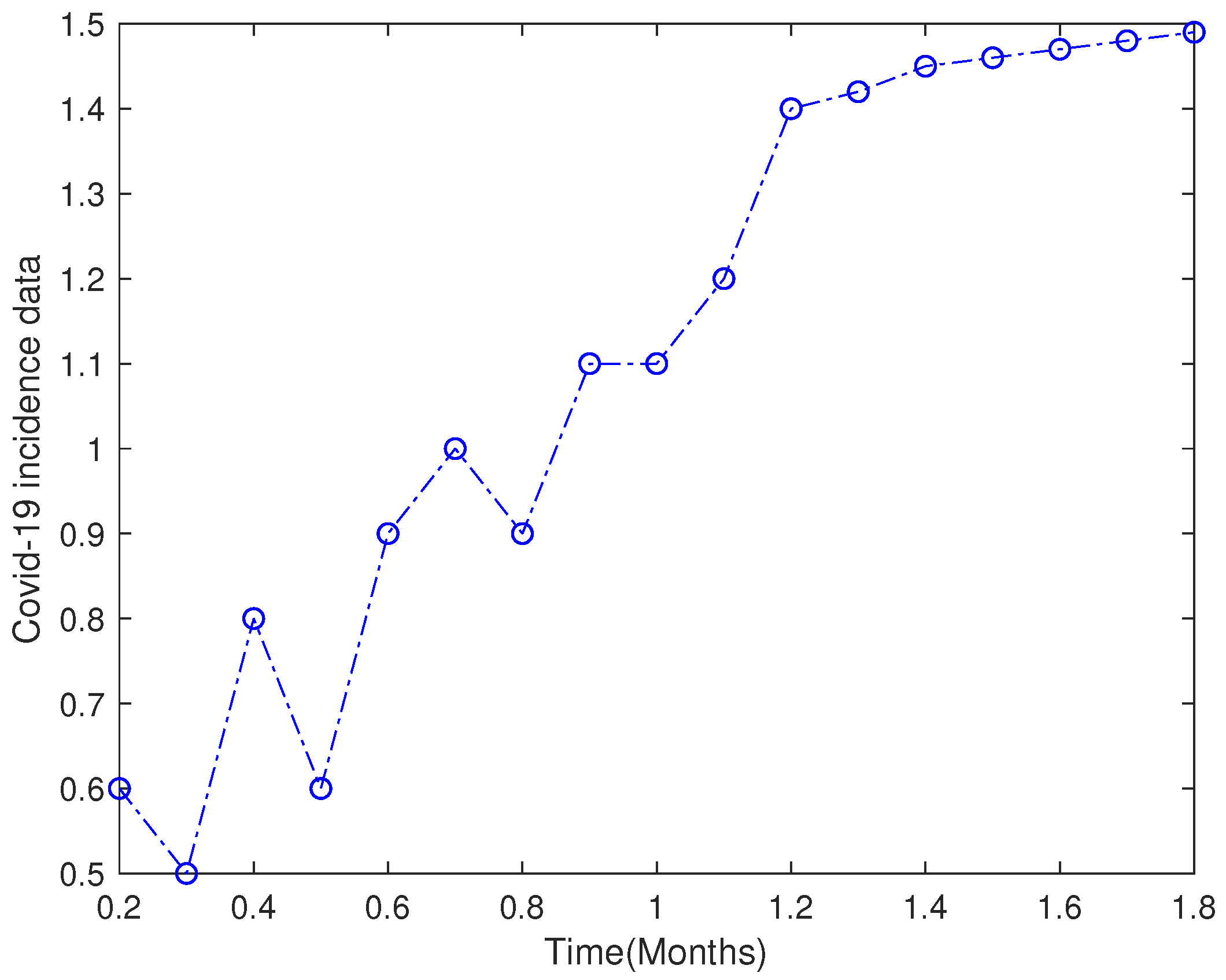
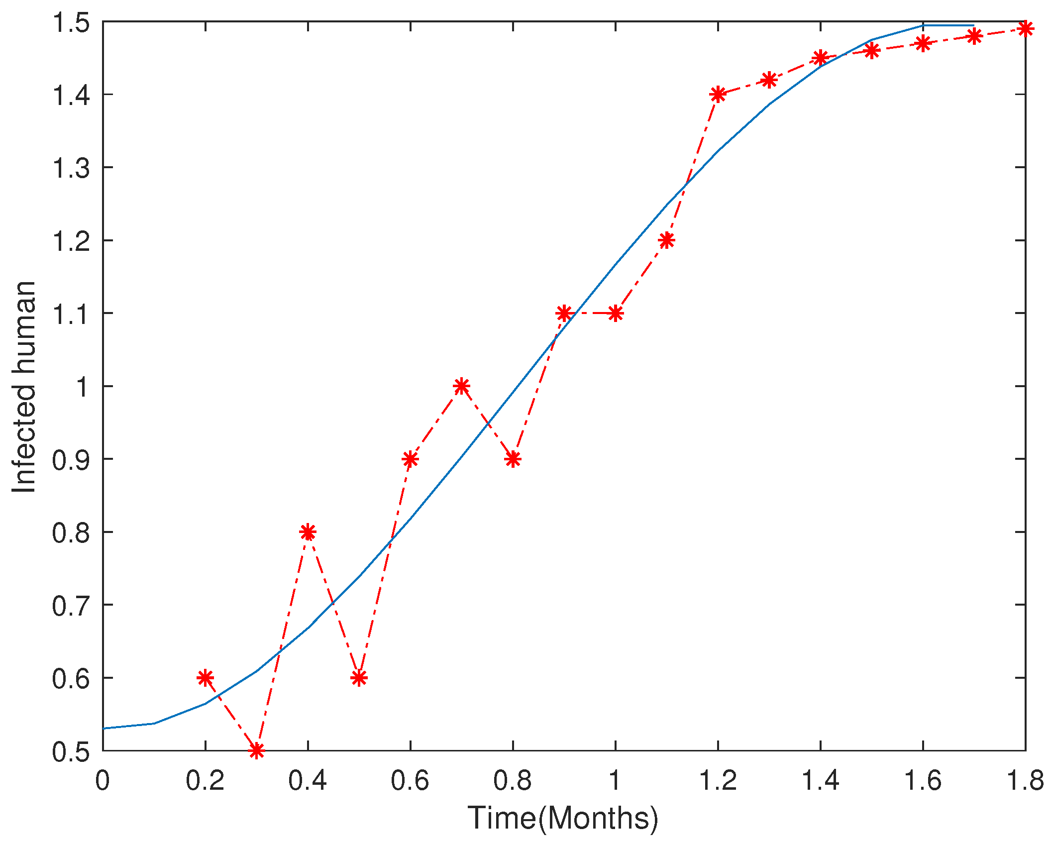
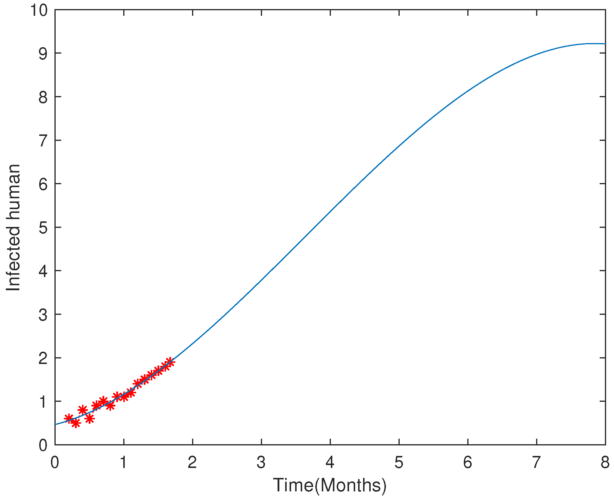
6.1. Case Study with Real Data: Khyber Pakhtunkhawa (Pakistan)

The Khyber Pakhtunkhawa Province, like other provinces of Pakistan and the rest of the world, is also being affected by COVID-19. We decided to calibrate our model with real data of COVID-19 from Khyber Pakhtunkhawa, Pakistan, from 9 April to 2 June 2020. For that, we have used the minimization method of MATLAB taking the initial weights

$$P\left(0\right)=\mathrm{35,525,047},I\left(0\right)=\mathrm{10,485},Q\left(0\right)=\mathrm{18,000},$$

determined from the work in [55], and $\theta =1$, from which we arrived to the values of the parameters shown in

Table 3. Parameter values for the case of Khyber Pakhtunkhawa, Pakistan.

Notation	Value	Reference
$\lambda$	0.028	[55]
$\gamma$	0.2	Estimated
$d_0$	0.011	[55]
$\mu$	0.2	Estimated
h	0.06	[55]
$\sigma$	0.04	Estimated
$\eta$	0.3	Estimated

.

Figure 2 shows the total number of individuals infected by COVID-19 as registered from 9 April to the 2nd in June 2020, which corresponds to the period of one month and 24 days used to calibrate our model.

Figure 3 compares the actual/real data of COVID-19 with the curve of infected given by Model (1), clearly showing the appropriateness of our model to describe the COVID-19 outbreak.

Figure 4 projects the long-term behavior of the COVID-19 outbreak during a period of eight months. We can see the data matches during the first 1.8 months and, additionally, we observe that the long-term behavior consists on a rise of infected individuals with time. This means that if the government did not apply proper strategies, the incidence could increase drastically in the coming months.

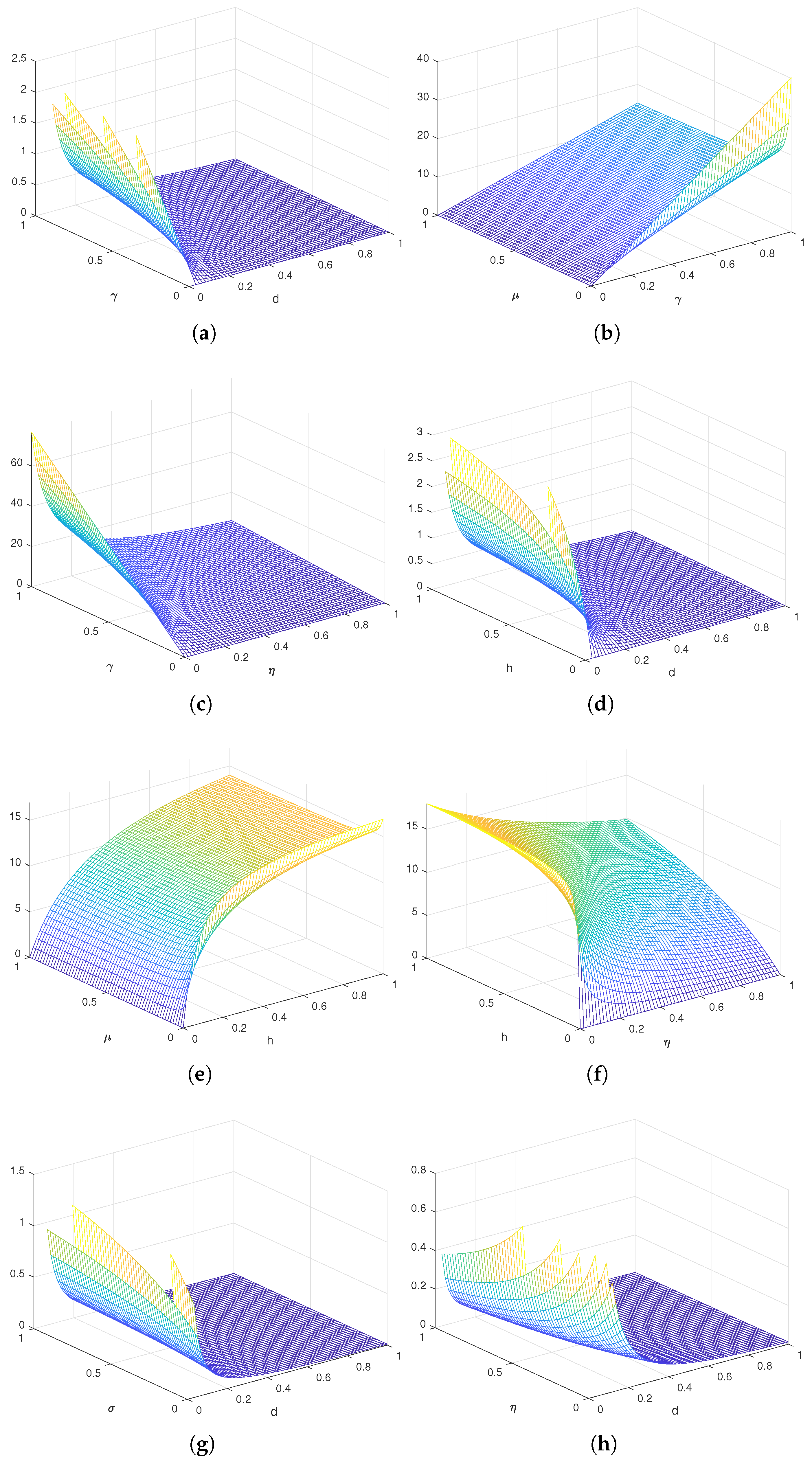
7. Sensitivity Analysis

Here, we conduct a sensitivity analysis to evaluate the parameters that are sensitive in minimizing the propagation of the ailment. Although its computation is tedious for complex biological models, forward sensitivity analysis is recorded as an important component of epidemic modeling: the ecologist and epidemiologist gain a lot of insight from the sensitivity study of the basic reproduction number $R_0$ [56]. In Definition 2, we assume that the basic reproduction number $R_0$ is differentiable with respect to parameter $\omega$. Given (3), this means that Definition 2 makes sense for $\omega \in \{\gamma ,\lambda ,d_0,\mu ,\sigma ,h,\eta \}$.

Definition 2.

The normalized forward sensitivity index of $R_0$ with respect to parameter ω is defined by

$$S_{\omega }=\frac{\omega }{R_0}\frac{\partial R_0}{\partial \omega }.$$

(27)

As we have an analytical form for the basic reproduction number, recall (3), we apply the direct differentiation process given in (27). Not only do the sensitivity indexes show us the impact of various factors associated with the spread of the infectious disease, but they also provide us with valuable details on the comparative change between $R_0$ and the parameters. Moreover, they also assist in the production of control strategies [57].

Table 4. Sensitivity indexes of the basic reproduction number $R_0$ (3) (see Definition 2) for relevant parameters of Model (1).

Parameters	Sensitivity	Value	Parameters	Sensitivity	Value
$\gamma$	$S_{\gamma }$	1.00000000	h	$S_h$	0.63636363
$d_0$	$S_{d_0}$	−1.48944805	$\mu$	$S_{\mu }$	−0.00974026
$\sigma$	$S_{\sigma }$	0.03165584	$\eta$	$S_{\eta }$	−0.16883117

demonstrates that $\gamma$, h, and $\sigma$ parameters have a positive effect on the basic reproduction number $R_0$, which means that the growth or decay of these parameters by 10% would increase or decrease the reproduction number by 10%, 6.36%, and 0.31%, respectively. On the other hand, $d_0$-, $\mu$-, and $\eta$-sensitive indexes indicate that increasing their values by 10% would decrease the basic reproduction number $R_0$ by 14.89%, 0.09%, and 1.68%, respectively.

The sensitivity of the basic reproduction number $R_0$ is also seen graphically in Figure 5.

8. Conclusions and Future Work

In this manuscript, we studied a COVID-19 disease model providing a detailed qualitative analysis and showed its usefulness with a case study of Khyber Pakhtunkhawa, Pakistan. Our sensitivity analysis shows that the transmission rate $\gamma$ has a huge effect on the model as compared to other parameters: the basic reproduction number varies directly with the transmission rate $\gamma$. The sensitivity analysis also showed that the death rate parameter $\mu$ has no effect on spreading the infection, which seems biologically correct. The transmission rate will be small by keeping a social distancing and self-quarantine situation that causes a decrease in the infection. In this way, one can control COVID-19 infection from rapid spreading in the community. In the future, we plan to analyze optimal control techniques to reduce the population of infected individuals by adopting a number of control measures. A modification of the given model is also possible by introducing more parameters for analyzing the early outbreaks of COVID-19 and then transmission and treatment aspects can be recalled. The given system can be also simulated by adding exposed and hospitalized classes and taking a stochastic fractional derivative. Here, we have provided a case study with real data from Pakistan, but other case studies can also be done.

References

1. Din, A.; Li, Y.; Khan, T.; Zaman, G. Mathematical analysis of spread and control of the novel corona virus (COVID-19) in China. Chaos Solitons Fractals 2020, 141, 110286. [Google Scholar] [CrossRef] [PubMed]
2. Din, A.; Khan, A.; Baleanu, D. Stationary distribution and extinction of stochastic coronavirus (COVID-19) epidemic model. Chaos Solitons Fractals 2020, 139, 110036. [Google Scholar] [CrossRef] [PubMed]
3. Koopmans, M.; Daszak, P.; Dedkov, V.G.; Dwyer, D.E.; Farag, E.; Fischer, T.K.; Hayman, D.T.S.; Leendertz, F.; Maeda, K.; Nguyen-Viet, H.; et al. Origins of SARS-CoV-2: Window is closing for key scientific studies. Nature 2021, 596, 482–485. [Google Scholar] [CrossRef] [PubMed]
4. Ndaïrou, F.; Area, I.; Nieto, J.J.; Silva, C.J.; Torres, D.F.M. Fractional model of COVID-19 applied to Galicia, Spain and Portugal. Chaos Solitons Fractals 2021, 144, 110652. [Google Scholar] [CrossRef] [PubMed]
5. Lemos-Paião, A.P.; Silva, C.J.; Torres, D.F.M. A New Compartmental Epidemiological Model for COVID-19 with a Case Study of Portugal. Ecol. Complex. 2020, 44, 100885. [Google Scholar] [CrossRef]
6. Zine, H.; Boukhouima, A.; Lotfi, E.M.; Mahrouf, M.; Torres, D.F.M.; Yousfi, N. A stochastic time-delayed model for the effectiveness of Moroccan COVID-19 deconfinement strategy. Math. Model. Nat. Phenom. 2020, 15, 50. [Google Scholar] [CrossRef]
7. Mahrouf, M.; Boukhouima, A.; Zine, H.; Lotfi, E.M.; Torres, D.F.M.; Yousfi, N. Modeling and Forecasting of COVID-19 Spreading by Delayed Stochastic Differential Equations. Axioms 2021, 10, 18. [Google Scholar] [CrossRef]
8. Ndaïrou, F.; Torres, D.F.M. Mathematical Analysis of a Fractional COVID-19 Model Applied to Wuhan, Spain and Portugal. Axioms 2021, 10, 135. [Google Scholar] [CrossRef]
9. Murray, J.D. Mathematical Biology I. An Introduction; Springer Science & Business Media: Berlin/Heidelberg, Germany, 2007. [Google Scholar]
10. Stewart, I.W. The Static and Dynamic Continuum Theory of Liquid Crystals; CRC Press: Boca Raton, FL, USA, 2019. [Google Scholar]
11. Samko, S.G.; Kilbas, A.A.; Marichev, O.I. Fractional Integrals and Derivatives; Gordon and Breach Science Publishers: Yverdon, Switzerland, 1993. [Google Scholar]
12. Toledo-Hernandez, R.; Rico-Ramirez, V.; Iglesias-Silva, G.A.; Diwekar, U.M. A Fractional calculus approach to the dynamic optimization of biological reactive systems. Part I: Fractional models for biological reactions. Chem. Eng. Sci. 2014, 117, 217–228. [Google Scholar] [CrossRef]
13. Miller, K.S.; Bertram, R. An Introduction to the Fractional Calculus and Fractional Differential Equations; Wiley-Interscience: New York, NY, USA, 1993. [Google Scholar]
14. Kilbas, A.A.; Srivastava, H.M.; Trujillo, J.J. Theory and Applications of Fractional Differential Equations; North-Holland Mathematics Studies; Elsevier Science B.V.: Amsterdam, The Netherlands, 2006; Volume 204. [Google Scholar]
15. Rahimy, M. Applications of fractional differential equations. Appl. Math. Sci. 2010, 4, 2453–2461. [Google Scholar] [CrossRef]
16. Rossikhin, Y.A.; Shitikova, M.V. Applications of fractional calculus to dynamic problems of linear and nonlinear hereditary mechanics of solids. Appl. Mech. Rev. 1997, 50, 15–67. [Google Scholar] [CrossRef]
17. Magin, R.L. Fractional Calculus in Bioengineering; Begell House: Redding, CA, USA, 2006. [Google Scholar]
18. Kamal, S.; Jarad, F.; Abdeljawad, T. On a nonlinear fractional order model of dengue fever disease under Caputo-Fabrizio derivative. Alex. Eng. J. 2020, 59, 2305–2313. [Google Scholar]
19. Biazar, J. Solution of the epidemic model by Adomian decomposition method. Appl. Math. Comput. 2006, 173, 1101–1106. [Google Scholar] [CrossRef]
20. Rafei, M.; Ganji, D.D.; Daniali, H. Solution of the epidemic model by homotopy perturbation method. Appl. Math. Comput. 2007, 187, 1056–1062. [Google Scholar] [CrossRef]
21. Abdelrazec, A. Adomian Decomposition Method: Convergence Analysis and Numerical Approximations. Master’s Thesis, McMaster University, Hamilton, ON, Canada, 2008. [Google Scholar]
22. Rezapour, S.; Mohammadi, H.; Jajarmi, A. A new mathematical model for Zika virus transmission. Adv. Differ. Equ. 2020, 2020, 1–15. [Google Scholar] [CrossRef]
23. Baleanu, D.; Ghanbari, B.; Asad, J.H.; Jajarmi, A.; Pirouz, H.M. Planar System-Masses in an Equilateral Triangle: Numerical Study within Fractional Calculus. Comput. Model. Eng. Sci. 2020, 124, 953–968. [Google Scholar] [CrossRef]
24. Jajarmi, A.; Baleanu, D. A New Iterative Method for the Numerical Solution of High-Order Non-linear Fractional Boundary Value Problems. Front. Phys. 2020, 8, 220. [Google Scholar] [CrossRef]
25. Sajjadi, S.S.; Baleanu, D.; Jajarmi, A.; Pirouz, H.M. A new adaptive synchronization and hyperchaos control of a biological snap oscillator. Chaos Solitons Fractals 2020, 138, 109919. [Google Scholar] [CrossRef]
26. Baleanu, D.; Jajarmi, A.; Sajjadi, S.S.; Asad, J.H. The fractional features of a harmonic oscillator with position-dependent mass. Commun. Theor. Phys. 2020, 72, 055002. [Google Scholar] [CrossRef]
27. Jajarmi, A.; Baleanu, D. On the fractional optimal control problems with a general derivative operator. Asian J. Control 2021, 23, 1062–1071. [Google Scholar] [CrossRef]
28. Azhar, I.; Siddiqui, M.J.; Muhi, I.; Abbas, M.; Akram, T. Nonlinear waves propagation and stability analysis for planar waves at far field using quintic B-spline collocation method. Alex. Eng. J. 2020, 59, 2695–2703. [Google Scholar]
29. Khalid, N.; Abbas, M.; Iqbal, M.K.; Singh, J.; Ismail, A.I. A computational approach for solving time fractional differential equation via spline functions. Alex. Eng. J. 2020, 59, 3061–3078. [Google Scholar] [CrossRef]
30. Akram, T.; Abbas, M.; Iqbal, A.; Baleanu, D.; Asad, J.H. Novel Numerical Approach Based on Modified Extended Cubic B-Spline Functions for Solving Non-Linear Time-Fractional Telegraph Equation. Symmetry 2020, 12, 1154. [Google Scholar] [CrossRef]
31. Din, A.; Li, Y. Controlling heroin addiction via age-structured modeling. Adv. Differ. Equ. 2020, 2020, 1–17. [Google Scholar] [CrossRef]
32. Akram, T.; Abbas, M.; Ali, A.; Iqbal, A.; Baleanu, D. A Numerical Approach of a Time Fractional Reaction–Diffusion Model with a Non-Singular Kernel. Symmetry 2020, 12, 1653. [Google Scholar] [CrossRef]
33. Amin, M.; Abbas, M.; Iqbal, M.K.; Baleanu, D. Numerical Treatment of Time-Fractional Klein–Gordon Equation Using Redefined Extended Cubic B-Spline Functions. Front. Phys. 2020, 8, 288. [Google Scholar] [CrossRef]
34. Amin, M.; Abbas, M.; Iqbal, M.K.; Ismail, A.I.M.; Baleanu, D. A fourth order non-polynomial quintic spline collocation technique for solving time fractional superdiffusion equations. Adv. Differ. Equ. 2019, 2019, 1–21. [Google Scholar] [CrossRef] [Green Version]
35. Khalid, N.; Abbas, M.; Iqbal, M.K. Non-polynomial quintic spline for solving fourth-order fractional boundary value problems involving product terms. Appl. Math. Comput. 2019, 349, 393–407. [Google Scholar] [CrossRef]
36. Iqbal, M.K.; Abbas, M.; Wasim, I. New cubic B-spline approximation for solving third order Emden-Flower type equations. Appl. Math. Comput. 2018, 331, 319–333. [Google Scholar] [CrossRef]
37. Akram, T.; Abbas, M.; Riaz, M.B.; Ismail, A.I.; Norhashidah, M.A. An efficient numerical technique for solving time fractional Burgers equation. Alex. Eng. J. 2020, 59, 2201–2220. [Google Scholar] [CrossRef]
38. Khalid, N.; Abbas, M.; Iqbal, M.K.; Baleanu, D. A numerical investigation of Caputo time fractional Allen-Cahn equation using redefined cubic B-spline functions. Adv. Differ. Equ. 2020, 2020, 1–22. [Google Scholar] [CrossRef]
39. Ndaïrou, F.; Torres, D.F.M. Pontryagin Maximum Principle for Distributed-Order Fractional Systems. Mathematics 2021, 9, 1883. [Google Scholar] [CrossRef]
40. Sabatier, J.; Agrawal, O.P.; Machado, J.A.T. Advances in Fractional Calculus; Springer: Dordrecht, The Netherlands, 2007. [Google Scholar] [CrossRef]
41. Baleanu, D.; Machado, J.A.T.; Albert, C.J. Fractional Dynamics and Control; Springer Science & Business Media: Berlin/Heidelberg, Germany, 2011. [Google Scholar]
42. Torres, D.F.M. Cauchy’s formula on nonempty closed sets and a new notion of Riemann-Liouville fractional integral on time scales. Appl. Math. Lett. 2021, 121, 107407. [Google Scholar] [CrossRef]
43. Al-Refai, M.; Abdeljawad, T. Analysis of the fractional diffusion equations with fractional derivative of non-singular kernel. Adv. Differ. Equ. 2017, 2017, 1–12. [Google Scholar] [CrossRef]
44. Mozyrska, D.; Torres, D.F.M.; Wyrwas, M. Solutions of systems with the Caputo-Fabrizio fractional delta derivative on time scales. Nonlinear Anal. Hybrid Syst. 2019, 32, 168–176. [Google Scholar] [CrossRef] [Green Version]
45. Abdeljawad, T. Fractional operators with exponential kernels and a Lyapunov type inequality. Adv. Differ. Equ. 2017, 2017, 1–11. [Google Scholar] [CrossRef] [Green Version]
46. Hasan, S.; El-Ajou, A.; Hadid, S.; Al-Smadi, M.; Momani, S. Atangana-Baleanu fractional framework of reproducing kernel technique in solving fractional population dynamics system. Chaos Solitons Fractals 2020, 133, 109624. [Google Scholar] [CrossRef]
47. Khan, S.A.; Shah, K.; Zaman, G.; Jarad, F. Existence theory and numerical solutions to smoking model under Caputo-Fabrizio fractional derivative. Chaos 2019, 29, 013128. [Google Scholar] [CrossRef] [PubMed]
48. Sidi Ammi, M.R.; Tahiri, M.; Torres, D.F.M. Necessary optimality conditions of a reaction-diffusion SIR model with ABC fractional derivatives. arXiv 2021, arXiv:2106.15055. [Google Scholar]
49. Din, A.; Li, Y.; Liu, Q. Viral dynamics and control of hepatitis B virus (HBV) using an epidemic model. Alex. Eng. J. 2020, 59, 667–679. [Google Scholar] [CrossRef]
50. Din, A.; Liang, J.; Zhou, T. Detecting critical transitions in the case of moderate or strong noise by binomial moments. Phys. Rev. E 2018, 98, 012114. [Google Scholar] [CrossRef]
51. Lai, C.C.; Shih, T.P.; Ko, W.C.; Tang, H.J.; Hsueh, P.R. Severe acute respiratory syndrome coronavirus 2 (SARS-CoV-2) and coronavirus disease-2019 (COVID-19): The epidemic and the challenges. Int. J. Antimicrob. Agents 2020, 55, 105924. [Google Scholar] [CrossRef] [PubMed]
52. Din, A.; Li, Y. Lévy noise impact on a stochastic hepatitis B epidemic model under real statistical data and its fractal–fractional Atangana–Baleanu order model. Phys. Scr. 2021, 96, 124008. [Google Scholar] [CrossRef]
53. Wang, J.; Shah, K.; Ali, A. Existence and Hyers-Ulam stability of fractional nonlinear impulsive switched coupled evolution equations. Math. Methods Appl. Sci. 2018, 41, 2392–2402. [Google Scholar] [CrossRef]
54. Ahmed, E.; El-Sayed, A.M.A.; El-Saka, H.A.A.; Ashry, G.A. On applications of Ulam-Hyers stability in biology and economics. arXiv 2010, arXiv:1004.1354. [Google Scholar]
55. Pakistan, G. COVID-19 Situation. Know about COVID-19, See the Realtime Pakistan and Worldwide. Available online: https://covid.gov.pk (accessed on 28 October 2021).
56. Rodrigues, H.S.; Monteiro, M.T.T.; Torres, D.F.M. Seasonality effects on dengue: Basic reproduction number, sensitivity analysis and optimal control. Math. Methods Appl. Sci. 2016, 39, 4671–4679. [Google Scholar] [CrossRef] [Green Version]
57. Rosa, S.; Torres, D.F.M. Parameter estimation, sensitivity analysis and optimal control of a periodic epidemic model with application to HRSV in Florida. Stat. Optim. Inf. Comput. 2018, 6, 139–149. [Google Scholar] [CrossRef] [Green Version]
Figure 1. Dynamical nature of susceptible, infected and quarantined individuals of the fractional ABC Model (1) for different values of the fractional-order θ . (a) P ( t ) —susceptible individuals along time t; (b) I ( t ) —infected individuals along time t; (c) Q ( t ) —quarantined individuals along time t.
Axioms 10 00290 g001
Figure 2. Real data of infected individuals by COVID-19 from Khyber Pakhtunkhwa, Pakistan, from 9 April to 2 June 2020.
Axioms 10 00290 g002
Figure 3. Comparison of infected individuals by COVID-19: Model (1) output (in blue) versus real data of Khyber Pakhtunkhawa, Pakistan, from 9 April to 2 June 2020 (in red).
Axioms 10 00290 g003
Figure 4. Real data of infected individuals by COVID-19 in Khyber Pakhtunkhwa, Pakistan (first 1.8 months, in red) and prediction from Model (1) during a period of 8 months (in blue).
Axioms 10 00290 g004
Figure 5. Sensitivity of the basic reproduction number R 0 (3) for relevant parameters of Model (1). (a) R 0 versus γ and d; (b) R 0 versus γ and μ ; (c) R 0 versus γ and η ; (d) R 0 versus h and d; (e) R 0 versus h and μ ; (f) R 0 versus h and η ; (g) R 0 versus d and σ ; (h) R 0 versus d and η .
Axioms 10 00290 g005