
Logic-Sensitivity of Aristotelian Diagrams in Non-Normal Modal Logics


Abstract
:1. Introduction
The standard modal square […] is valid with respect to any modal system at least as strong as the deontic system , but invalid in any normal system strictly weaker than .([44], p. 313, emphasis added)
2. Technical Background
2.1. Modal Logic
| iff | ||
| iff |  | |
| iff | and | |
| iff | for all: ifthen. |
| iff | iff | |||||
| iff | iff |
| iff | . |
- For every augmented neighborhood frame , there exists a modally equivalent Kripke frame , that is, for all valuations , states and formulas we have if ;
- For every Kripke frame , there exists a modally equivalent augmented neighborhood frame , that is, for all valuations , states and formulas we have if .
| iff | iff | |||||
| iff | iff | |||||
| iff | iff |
2.2. Logical Geometry
| -contradictory | iff | and | ||
| -contrary | iff | and | 
| |
| -subcontrary | iff |
| and | |
| in -subalternation | iff | and |
|
, (ii) , (iii) and (iv) .- iff , for all Aristotelian relations R,
- iff .
).2.3. Bitstring Semantics
3. Logic-Sensitivity and Aristotelian Families
3.1. Introduction
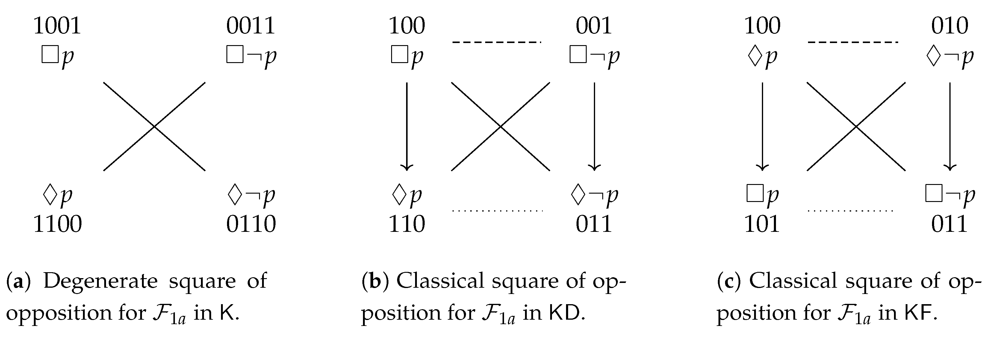
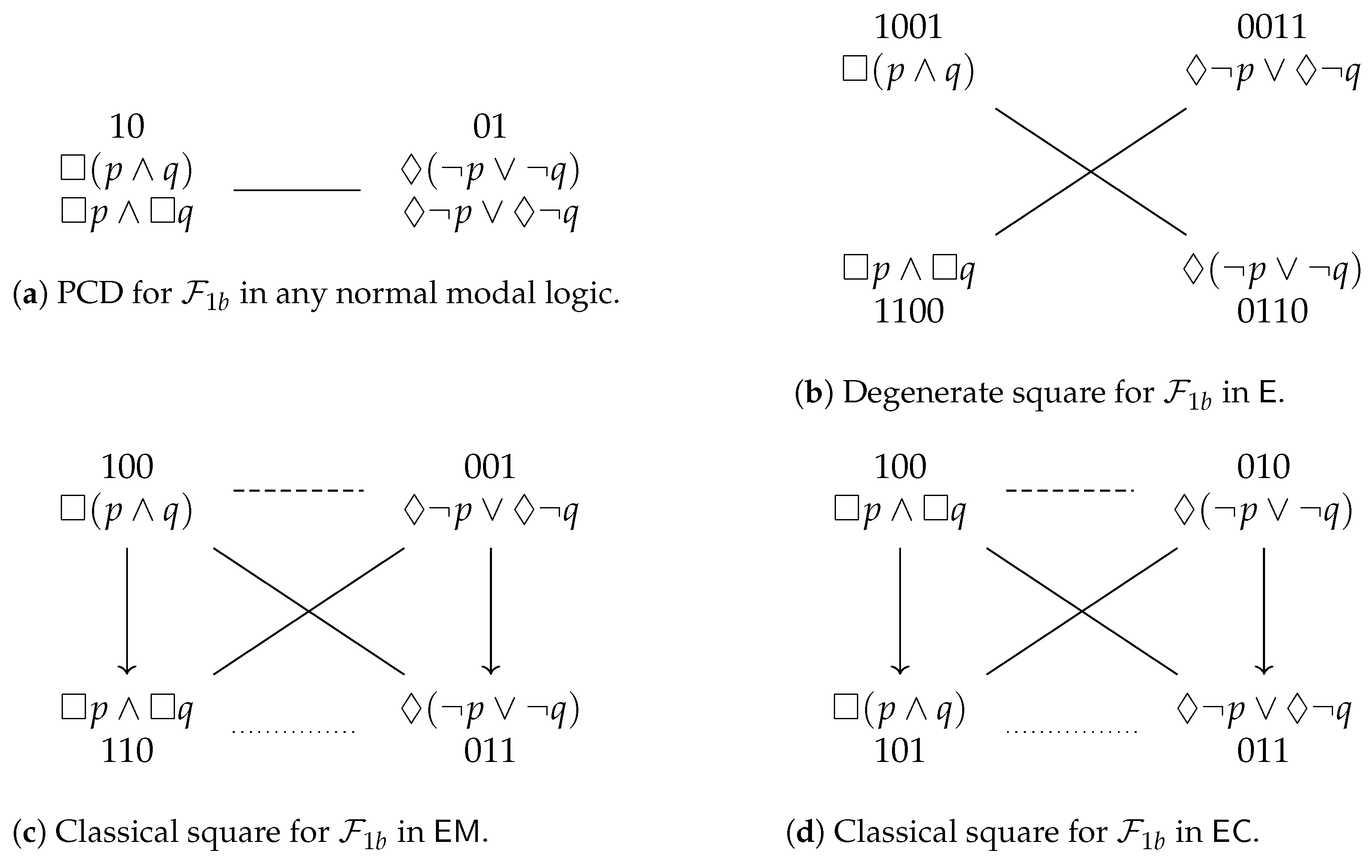
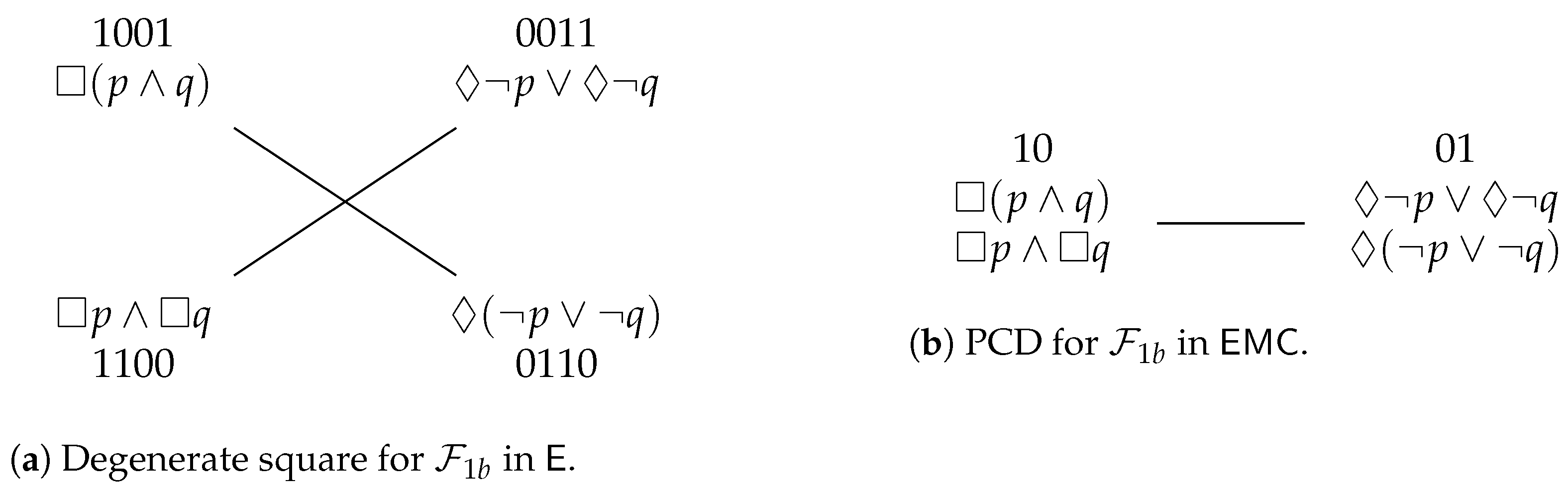
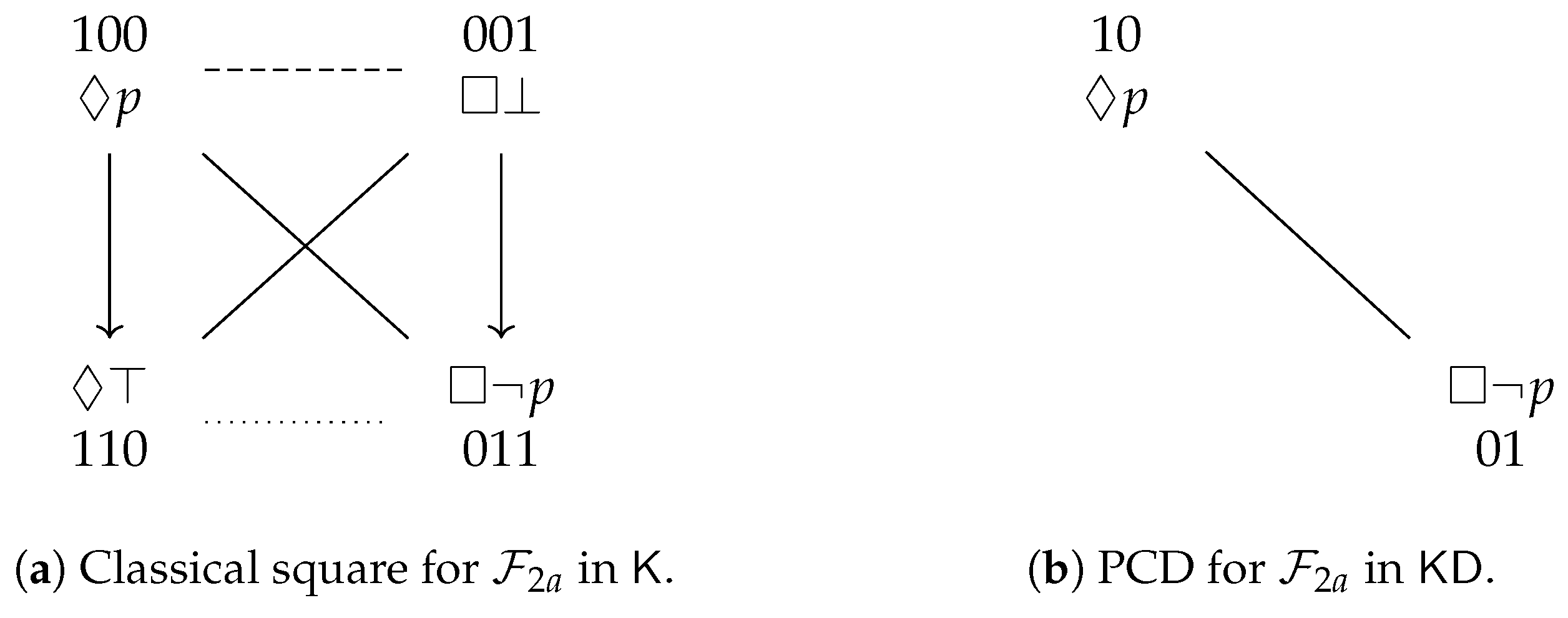
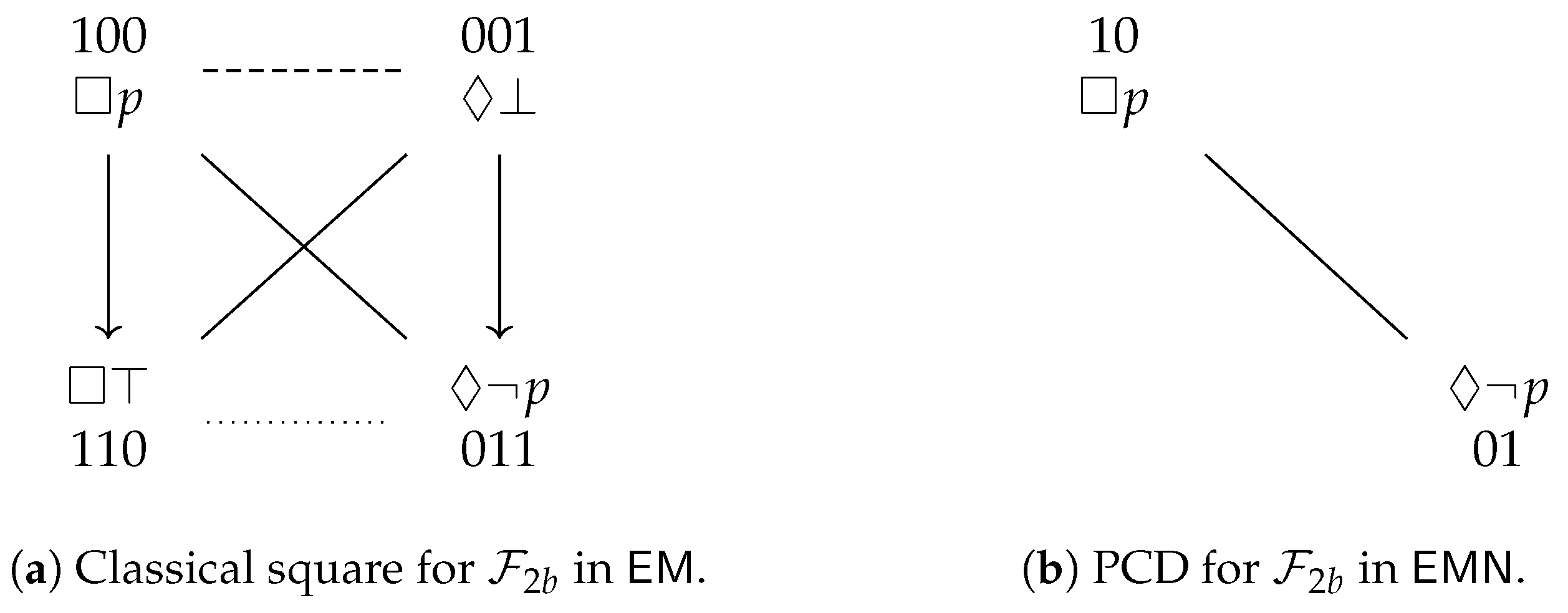
), but in the modal logic , these same two formulas are contradictory to each other (since and also ). Or to give an example from non-normal modal logic: it is straightforward to check that the formulas and are contraries in , but subcontraries in .3.2. Examples from Normal Modal Logic
. To summarize, the Aristotelian diagram for is a degenerate square of opposition, which was already shown in Figure 1b, and is repeated here in Figure 3a, for the sake of reference. An easy computation yields the partition that is induced by in :. To summarize, the Aristotelian diagram for is a classical square of opposition, which was already shown in Figure 1a, and is repeated here in Figure 3b, for the sake of reference. It is straightforward to check that there does not exist an Aristotelian isomorphism between and , which means that we have obtained our first concrete example of the logic-sensitivity of Aristotelian diagrams with respect to Aristotelian families. Furthermore, an easy computation yields the partition that is induced by in :3.3. Examples from Non-Normal Modal Logic
4. Logic-Sensitivity and Logical Equivalence of Formulas
4.1. Introduction
4.2. Examples from Normal Modal Logic
4.3. Examples from Non-Normal Modal Logic
4.4. Theory and Further Examples
- 1.
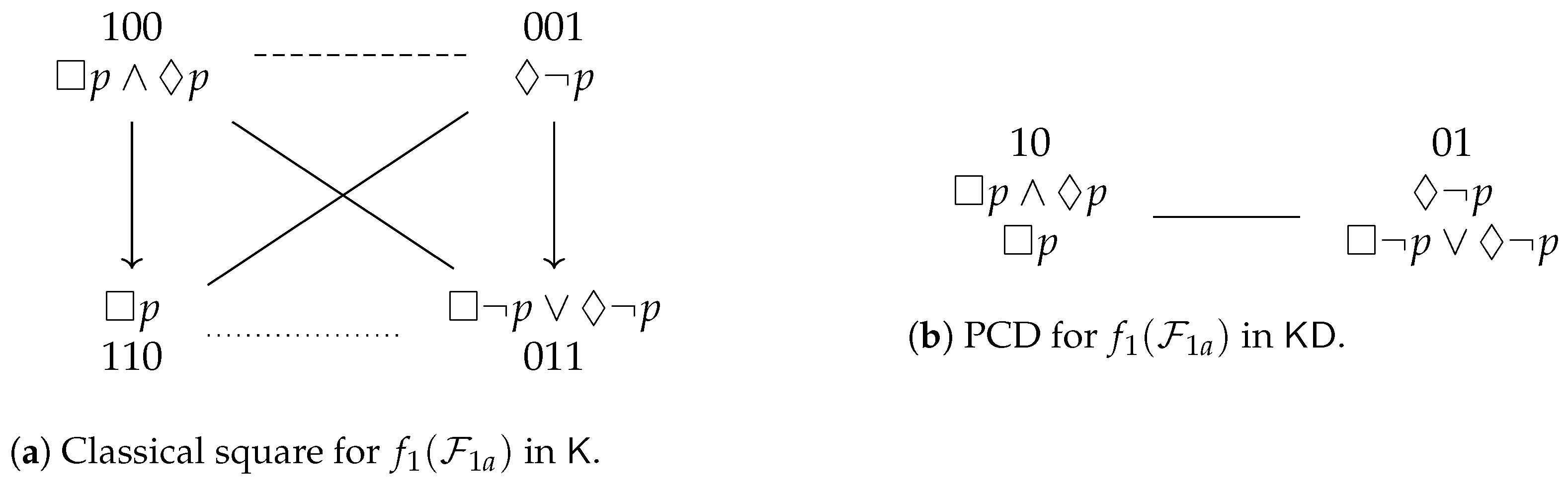
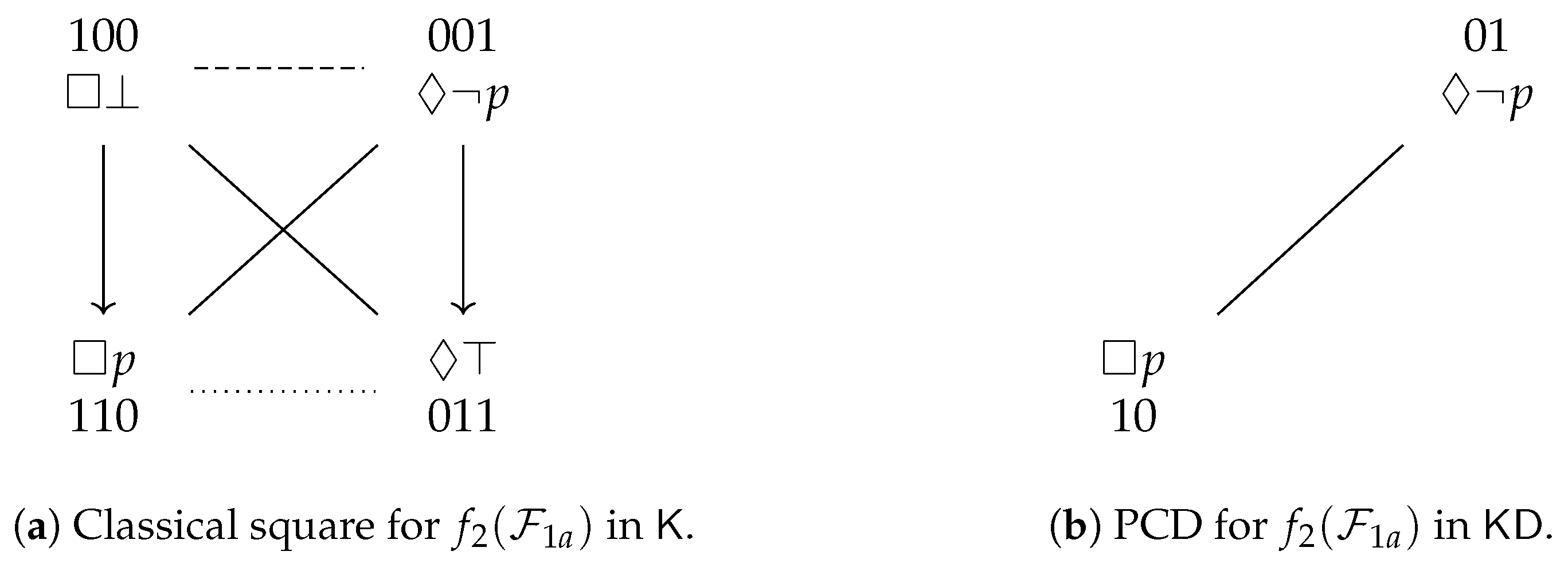
- If the Aristotelian diagram for is a degenerate square, then the Aristotelian diagram for is a classical square (with an -subalternation from to α);
- 2.
- If the Aristotelian diagram for is a classical square (with an -subalternation from α to β), then the Aristotelian diagram for is a PCD (with ).
5. Logic-Sensitivity and Contingency of Formulas
5.1. Introduction
5.2. Examples from Normal Modal Logic
5.3. Examples from Non-Normal Modal Logic
. Furthermore, the partition that is induced by in looks as follows:5.4. Theory and Further Examples
- 1.
- If the Aristotelian diagram for is a degenerate square, then the Aristotelian diagram for is a classical square (with an -subalternation from to α);
- 2.
- If the Aristotelian diagram for is a classical square (with an -subalternation from α to β), then and are not -contingent and the Aristotelian diagram for is a PCD.
6. Logic-Sensitivity and Boolean Subfamilies
6.1. Introduction
6.2. Theory and Examples
- 1.
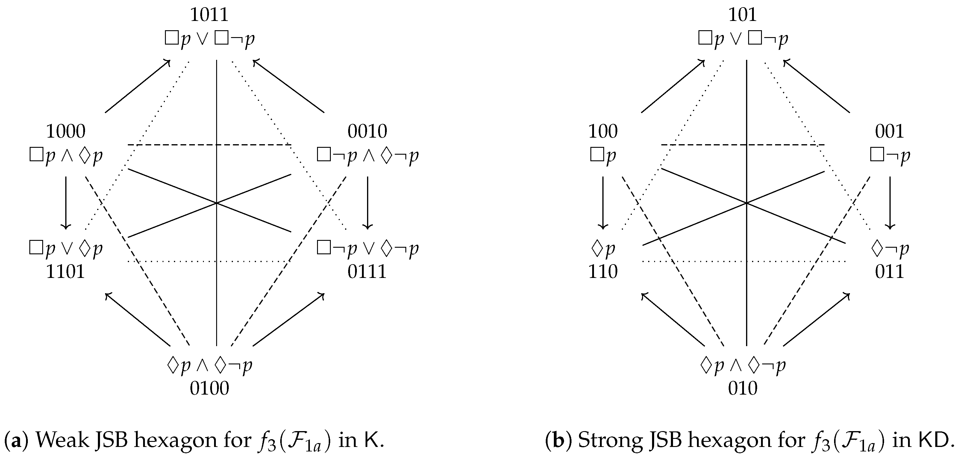
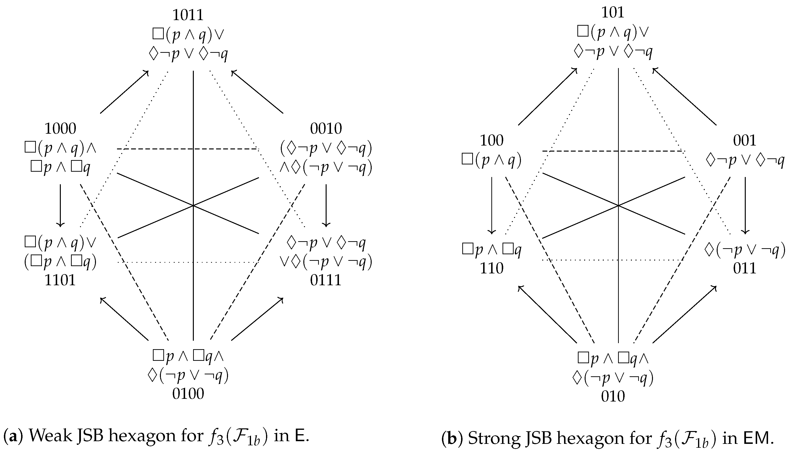
- If the Aristotelian diagram for is a degenerate square, then the Aristotelian diagram for is a weak JSB hexagon (with pairwise -contrarieties between , and );
- 2.
- If the Aristotelian diagram for is a classical square (with an -subalternation from α to β), then the Aristotelian diagram for is a strong JSB hexagon (with the same pairwise -contrarieties).
7. Conclusions
- If and are both degenerate squares, then is a weak Buridan octagon;
- If exactly one of and is a degenerate square and the other is a classical square, then is an intermediate Buridan octagon;
- If and are both classical squares, then is a strong Buridan octagon.
Funding
Institutional Review Board Statement
Informed Consent Statement
Data Availability Statement
Acknowledgments
Conflicts of Interest
References
- Parsons, T. The Traditional Square of Opposition. In Stanford Encyclopedia of Philosophy (Summer 2017 Edition); Zalta, E.N., Ed.; CSLI: Stanford, CA, USA, 2017. [Google Scholar]
- Jaspers, D.; Seuren, P. The Square of Opposition in Catholic Hands: A Chapter in the History of 20th-Century Logic. Log. Anal. 2016, 59, 1–35. [Google Scholar]
- Pozzi, L. Studi di Logica Antica e Medioevale; Liviana Editrice: Padova, Italy, 1974. [Google Scholar]
- Ciucci, D.; Dubois, D.; Prade, H. Oppositions in Rough Set Theory. In Rough Sets and Knowledge Technology; Li, T., Nguyen, H.S., Wang, G., Grzymala-Busse, J., Janicki, R., Hassanien, A.E., Yu, H., Eds.; Springer: Berlin/Heidelberg, Germany, 2012; pp. 504–513. [Google Scholar]
- Ciucci, D.; Dubois, D.; Prade, H. The Structure of Oppositions in Rough Set Theory and Formal Concept Analysis—Toward a New Bridge between the Two Settings. In Foundations of Information and Knowledge Systems (FoIKS 2014); Beierle, C., Meghini, C., Eds.; Springer: Berlin/Heidelberg, Germany, 2014; pp. 154–173. [Google Scholar]
- Yao, Y. Duality in Rough Set Theory Based on the Square of Opposition. Fundam. Inform. 2013, 127, 49–64. [Google Scholar] [CrossRef]
- Dubois, D.; Prade, H. From Blanché’s Hexagonal Organization of Concepts to Formal Concept Analysis and Possibility Theory. Log. Universalis 2012, 6, 149–169. [Google Scholar] [CrossRef]
- Dubois, D.; Prade, H. Formal Concept Analysis from the Standpoint of Possibility Theory. In Formal Concept Analysis (ICFCA 2015); Baixeries, J., Sacarea, C., Ojeda-Aciego, M., Eds.; Springer: Berlin/Heidelberg, Germany, 2015; pp. 21–38. [Google Scholar]
- Dubois, D.; Prade, H. Possibilistic Logic: From Certainty-Qualified Statements to Two-Tiered Logics—A Prospective Survey. In Logics in Artificial Intelligence (JELIA 2019); Calimeri, F., Leona, N., Manna, M., Eds.; Springer: Berlin/Heidelberg, Germany, 2019; pp. 3–20. [Google Scholar]
- Amgoud, L.; Besnard, P.; Hunter, A. Foundations for a Logic of Arguments. In Logical Reasoning and Computation: Essays Dedicated to Luis Fariñas del Cerro; Cabalar, P., Herzig, M.D.A., Pearce, D., Eds.; IRIT: Toulouse, France, 2016; pp. 95–107. [Google Scholar]
- Amgoud, L.; Prade, H. Can AI Models Capture Natural Language Argumentation? Int. J. Cogn. Inform. Nat. Intell. 2012, 6, 19–32. [Google Scholar] [CrossRef] [Green Version]
- Amgoud, L.; Prade, H. Towards a Logic of Argumentation. In Scalable Uncertainty Management 2012; Hüllermeier, E., Ed.; Springer: Berlin/Heidelberg, Germany, 2012; pp. 558–565. [Google Scholar]
- Amgoud, L.; Prade, H. Amgoud, L.; Prade, H. A Formal Concept View of Formal Argumentation. In Symbolic and Quantitative Approaches to Reasoning with Uncertainty (ECSQARU 2013); van der Gaag, L.C., Ed.; Springer: Berlin/Heidelberg, Germany, 2013; pp. 1–12. [Google Scholar]
- Ciucci, D.; Dubois, D.; Prade, H. Structures of Opposition in Fuzzy Rough Sets. Fundam. Inform. 2015, 142, 1–19. [Google Scholar] [CrossRef]
- Ciucci, D.; Dubois, D.; Prade, H. Structures of Opposition Induced by Relations. The Boolean and the Gradual Cases. Ann. Math. Artif. Intell. 2016, 76, 351–373. [Google Scholar] [CrossRef] [Green Version]
- Dubois, D.; Prade, H. Gradual Structures of Oppositions. In Enric Trillas: A Passion for Fuzzy Sets; Magdalena, L., Verdegay, J.L., Esteva, F., Eds.; Springer: Berlin/Heidelberg, Germany, 2015; pp. 79–91. [Google Scholar]
- Dubois, D.; Prade, H.; Rico, A. Graded Cubes of Opposition and Possibility Theory with Fuzzy Events. Int. J. Approx. Reason. 2017, 84, 168–185. [Google Scholar] [CrossRef] [Green Version]
- Miclet, L.; Prade, H. Analogical Proportions and Square of Oppositions. In Information Processing and Management of Uncertainty in Knowledge-Based Systems 2014, Part II; Laurent, A., Ed.; Springer: Berlin/Heidelberg, Germany, 2014; pp. 324–334. [Google Scholar]
- Prade, H.; Richard, G. From Analogical Proportion to Logical Proportions. Log. Universalis 2013, 7, 441–505. [Google Scholar] [CrossRef] [Green Version]
- Prade, H.; Richard, G. Picking the one that does not fit – A matter of logical proportions. In Proceedings of the 8th Conference of the European Society for Fuzzy Logic and Technology (EUSFLAT-13), Milan, Italy, 11–13 September 2013; Pasi, G., Montero, J., Ciucci, D., Eds.; Atlantis Press: Amsterdam, The Netherlands, 2013; pp. 392–399. [Google Scholar]
- Prade, H.; Richard, G. On Different Ways to be (dis)similar to Elements in a Set. Boolean Analysis and Graded Extension. In Information Processing and Management of Uncertainty in Knowledge-Based Systems 2016, Part II; Carvalho, J.P., Ed.; Springer: Berlin/Heidelberg, Germany, 2016; pp. 605–618. [Google Scholar]
- Prade, H.; Richard, G. From the Structures of Opposition Between Similarity and Dissimilarity Indicators to Logical Proportions. In Representation and Reality in Humans, Other Living Organisms and Intelligent Machines; Dodig-Crnkovic, G., Giovagnoli, R., Eds.; Springer: Berlin/Heidelberg, Germany, 2017; pp. 279–299. [Google Scholar]
- Dubois, D.; Prade, H.; Rico, A. Structures of Opposition and Comparisons: Boolean and Gradual Cases. Log. Universalis 2020, 14, 115–149. [Google Scholar] [CrossRef]
- Gilio, A.; Pfeifer, N.; Sanfilippo, G. Transitivity in Coherence-Based Probability Logic. J. Appl. Log. 2016, 14, 46–64. [Google Scholar] [CrossRef]
- Pfeifer, N.; Sanfilippo, G. Square of Opposition under Coherence. In Soft Methods for Data Science; Ferraro, M.B., Ed.; Springer: Berlin/Heidelberg, Germany, 2017; pp. 407–414. [Google Scholar]
- Pfeifer, N.; Sanfilippo, G. Probabilistic Squares and Hexagons of Opposition under Coherence. Int. J. Approx. Reason. 2017, 88, 282–294. [Google Scholar] [CrossRef] [Green Version]
- Dubois, D.; Prade, H.; Rico, A. The Cube of Opposition—A Structure underlying many Knowledge Representation Formalisms. In Proceedings of the Twenty-Fourth International Joint Conference on Artificial Intelligence (IJCAI 2015), Buenos Aires, Argentina, 25–31 July 2015; Yang, Q., Wooldridge, M., Eds.; AAAI Press: Palo Alto, CA, USA, 2015; pp. 2933–2939. [Google Scholar]
- Dubois, D.; Prade, H.; Rico, A. The Cube of Opposition and the Complete Appraisal of Situations by Means of Sugeno Integrals. In Foundations of Intelligent Systems (ISMIS 2015); Esposito, F., Ed.; Springer: Berlin/Heidelberg, Germany, 2015; pp. 197–207. [Google Scholar]
- Dubois, D.; Prade, H.; Rico, A. Organizing Families of Aggregation Operators into a Cube of Opposition. In Granular, Soft and Fuzzy Approaches for Intelligent Systems; Kacprzyk, J., Filev, D., Beliakov, G., Eds.; Springer: Berlin/Heidelberg, Germany, 2017; pp. 27–45. [Google Scholar]
- Londey, D.; Johanson, C. Apuleius and the Square of Opposition. Phronesis 1984, 29, 165–173. [Google Scholar]
- Correia, M. Boethius on the Square of Opposition. In Around and Beyond the Square of Opposition; Béziau, J.Y., Jacquette, D., Eds.; Springer: Basel, Switzerland, 2012; pp. 41–52. [Google Scholar]
- Lemaire, J. Is Aristotle the Father of the Square of Opposition? In New Dimensions of the Square of Opposition; Béziau, J.Y., Gerogiorgakis, S., Eds.; Philosophia Verlag: Munich, Germany, 2017; pp. 33–69. [Google Scholar]
- Correia, M. Aristotle’s Squares of Opposition. S. Am. J. Log. 2017, 3, 313–326. [Google Scholar]
- Knuuttila, S. Medieval Theories of Modality. In Stanford Encyclopedia of Philosophy (Summer 2017 Edition); Zalta, E.N., Ed.; CSLI: Stanford, CA, USA, 2017. [Google Scholar]
- Geudens, C.; Demey, L. On the Aristotelian Roots of the Modal Square of Opposition. 2021; Submitted. [Google Scholar]
- Geudens, C.; Demey, L. Modal Logic in the Post-Medieval Period. The Case of John Fabri (c. 1500). 2021; Submitted. [Google Scholar]
- Konyndyk, K. Introductory Modal Logic; University of Notre Dame Press: Notre Dame, IN, USA, 1986. [Google Scholar]
- Fitting, M.; Mendelsohn, R.L. First-Order Modal Logic; Kluwer: Dordrecht, The Netherlands, 1998. [Google Scholar]
- Carnielli, W.; Pizzi, C. Modalities and Multimodalities; Springer: Dordrecht, The Netherlands, 2008. [Google Scholar]
- Łukasiewicz, J. A System of Modal Logic. In Selected Works; Borkowski, L., Ed.; North Holland Publishing Company: Amsterdam, The Netherlands, 1970; pp. 352–390. [Google Scholar]
- Béziau, J.Y. Paraconsistent logic from a modal viewpoint. J. Appl. Log. 2005, 3, 7–14. [Google Scholar] [CrossRef] [Green Version]
- Marcos, J. Nearly Every Normal Modal Logic is Paranormal. Log. Anal. 2005, 48, 279–300. [Google Scholar]
- Woleński, J. Applications of Squares of Oppositions and Their Generalizations in Philosophical Analysis. Log. Universalis 2008, 2, 13–29. [Google Scholar] [CrossRef]
- Pizzi, C. Generalization and Composition of Modal Squares of Opposition. Log. Universalis 2016, 10, 313–325. [Google Scholar] [CrossRef]
- Luzeaux, D.; Sallantin, J.; Dartnell, C. Logical Extensions of Aristotle’s Square. Log. Universalis 2008, 2, 167–187. [Google Scholar] [CrossRef] [Green Version]
- Moretti, A. The Geometry of Logical Opposition. Ph.D. Thesis, University of Neuchâtel, Neuchâtel, Switzerland, 2009. [Google Scholar]
- Smessaert, H. On the 3D Visualisation of Logical Relations. Log. Universalis 2009, 3, 303–332. [Google Scholar] [CrossRef]
- Demey, L. Structures of Oppositions for Public Announcement Logic. In Around and Beyond the Square of Opposition; Béziau, J.Y., Jacquette, D., Eds.; Springer: Basel, Switzerland, 2012; pp. 313–339. [Google Scholar]
- Smessaert, H.; Demey, L. Béziau’s Contributions to the Logical Geometry of Modalities and Quantifiers. In The Road to Universal Logic; Koslow, A., Buchsbaum, A., Eds.; Springer: Basel, Switzerland, 2015; pp. 475–493. [Google Scholar]
- Demey, L.; Smessaert, H. Aristotelian and Duality Relations Beyond the Square of Opposition. In Diagrammatic Representation and Inference; Chapman, P., Stapleton, G., Moktefi, A., Perez-Kriz, S., Bellucci, F., Eds.; Springer: Berlin/Heidelberg, Germany, 2018; pp. 640–656. [Google Scholar]
- Smessaert, H.; Demey, L. Logical Geometries and Information in the Square of Opposition. J. Logic Lang. Inf. 2014, 23, 527–565. [Google Scholar] [CrossRef]
- Demey, L. Interactively Illustrating the Context-Sensitivity of Aristotelian Diagrams. In Modeling and Using Context; Christiansen, H., Stojanovic, I., Papadopoulos, G., Eds.; Springer: Berlin/Heidelberg, Germany, 2015; pp. 331–345. [Google Scholar]
- Demey, L.; Smessaert, H. Logical and Geometrical Distance in Polyhedral Aristotelian Diagrams in Knowledge Representation. Symmetry 2017, 9, 204. [Google Scholar] [CrossRef] [Green Version]
- Demey, L. Computing the Maximal Boolean Complexity of Families of Aristotelian Diagrams. J. Log. Comput. 2018, 28, 1323–1339. [Google Scholar] [CrossRef]
- Demey, L.; Smessaert, H. Geometric and Cognitive Differences between Aristotelian Diagrams for the Boolean Algebra B4. Ann. Math. Artif. Intell. 2018, 83, 185–208. [Google Scholar] [CrossRef]
- Demey, L. Metalogic, Metalanguage and Logical Geometry. Log. Anal. 2019, 248, 453–478. [Google Scholar]
- Demey, L.; Smessaert, H. Combinatorial Bitstring Semantics for Arbitrary Logical Fragments. J. Philos. Log. 2018, 47, 325–363. [Google Scholar] [CrossRef] [Green Version]
- Demey, L.; Smessaert, H. Using Multigraphs to Study the Interaction Between Opposition, Implication and Duality Relations in Logical Squares. In Diagrammatic Representation and Inference; Pietarinen, A.V., Chapman, P., Bosveld-de Smet, L., Giardino, V., Corter, J., Linker, S., Eds.; Springer: Berlin/Heidelberg, Germany, 2020; pp. 385–393. [Google Scholar]
- Smessaert, H.; Shimojima, A.; Demey, L. Free Rides in Logical Space Diagrams Versus Aristotelian Diagrams. In Diagrammatic Representation and Inference; Pietarinen, A.V., Chapman, P., Bosveld-de Smet, L., Giardino, V., Corter, J., Linker, S., Eds.; Springer: Berlin/Heidelberg, Germany, 2020; pp. 419–435. [Google Scholar]
- Demey, L. Aristotelian Diagrams for Semantic and Syntactic Consequence. Synthese 2021, 198, 187–207. [Google Scholar] [CrossRef]
- Pacuit, E. Neighborhood Semantics for Modal Logic; Springer: Cham, Switzerland, 2017. [Google Scholar]
- Segerberg, K. An Essay in Classical Modal Logic; Uppsala Universitet: Uppsala, Sweden, 1971. [Google Scholar]
- Chellas, B.F. Modal Logic. An Introduction; Cambridge University Press: Cambridge, UK, 1980. [Google Scholar]
- Demey, L.; Smessaert, H. The Relationship between Aristotelian and Hasse Diagrams. In Diagrammatic Representation and Inference; Dwyer, T., Purchase, H., Delaney, A., Eds.; Springer: Berlin/Heidelberg, Germany, 2014; pp. 213–227. [Google Scholar]
- Demey, L. Boolean Considerations on John Buridan’s Octagons of Oppositions. Hist. Philos. Log. 2019, 40, 116–134. [Google Scholar] [CrossRef]
- Jacoby, P. A Triangle of Opposites for Types of Propositions in Aristotelian Logic. New Scholast. 1950, 24, 32–56. [Google Scholar] [CrossRef]
- Sesmat, A. Logique II. Les Raisonnements. La Syllogistique; Hermann: Paris, France, 1951. [Google Scholar]
- Blanché, R. Structures Intellectuelles; Vrin: Paris, France, 1966. [Google Scholar]
- Pellissier, R. Setting n-Opposition. Log. Universalis 2008, 2, 235–263. [Google Scholar] [CrossRef]
- Smessaert, H.; Demey, L. The Unreasonable Effectiveness of Bitstrings in Logical Geometry. In The Square of Opposition: A Cornerstone of Thought; Béziau, J.Y., Basti, G., Eds.; Springer: Basel, Switzerland, 2017; pp. 197–214. [Google Scholar]
- Demey, L. Aristotelian Diagrams in the Debate on Future Contingents. Sophia 2019, 58, 321–329. [Google Scholar] [CrossRef]
- Wong, W.; Vennekens, J.; Schaeken, W.; Demey, L. Extending Knowledge Space Theory to contingent information with bitstring semantics. In Proceedings of the MathPsych/ICCM 2021—Annual Joint Meeting of the Society for Mathematical Psychology and the International Conference on Cognitive Modeling, Online, 1–12 July 2021. [Google Scholar]
- Wong, W.; Vennekens, J.; Demey, L.; Schaeken, W. Complexity Evaluation on Different DMN Table Representations with Bitstring Semantics. In Proceedings of the 54th Hawaii International Conference on System Sciences, Seattle, WA, USA, 5–8 January 2021. [Google Scholar]
- Hansen, H.H. Monotonic Modal Logics. Master’s Thesis, ILLC, Universiteit van Amsterdam, Amsterdam, The Netherlands, 2003. [Google Scholar]


Publisher’s Note: MDPI stays neutral with regard to jurisdictional claims in published maps and institutional affiliations. |
© 2021 by the author. Licensee MDPI, Basel, Switzerland. This article is an open access article distributed under the terms and conditions of the Creative Commons Attribution (CC BY) license (https://creativecommons.org/licenses/by/4.0/).
Share and Cite
Demey, L. Logic-Sensitivity of Aristotelian Diagrams in Non-Normal Modal Logics. Axioms 2021, 10, 128. https://doi.org/10.3390/axioms10030128
Demey L. Logic-Sensitivity of Aristotelian Diagrams in Non-Normal Modal Logics. Axioms. 2021; 10(3):128. https://doi.org/10.3390/axioms10030128
Chicago/Turabian StyleDemey, Lorenz. 2021. "Logic-Sensitivity of Aristotelian Diagrams in Non-Normal Modal Logics" Axioms 10, no. 3: 128. https://doi.org/10.3390/axioms10030128
APA StyleDemey, L. (2021). Logic-Sensitivity of Aristotelian Diagrams in Non-Normal Modal Logics. Axioms, 10(3), 128. https://doi.org/10.3390/axioms10030128