
Analyzing Uncertain Dynamical Systems after State-Space Transformations into Cooperative Form: Verification of Control and Fault Diagnosis


Abstract
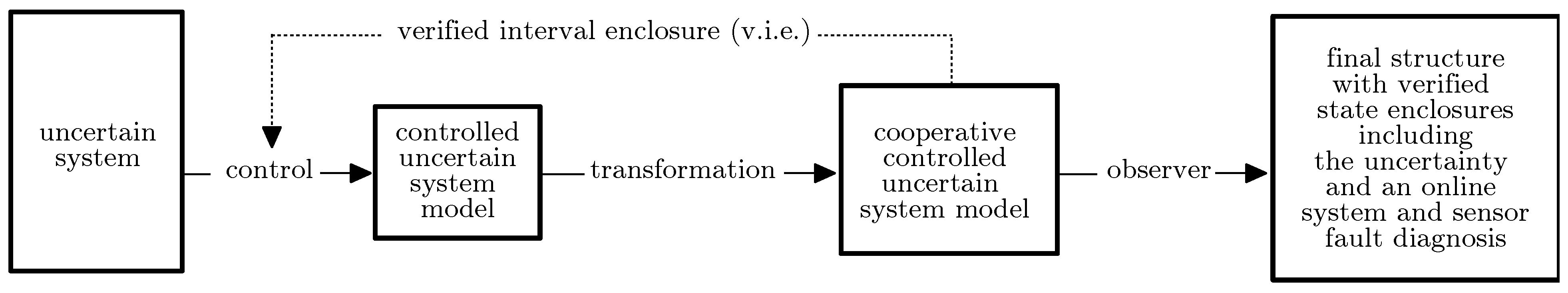
1. Introduction
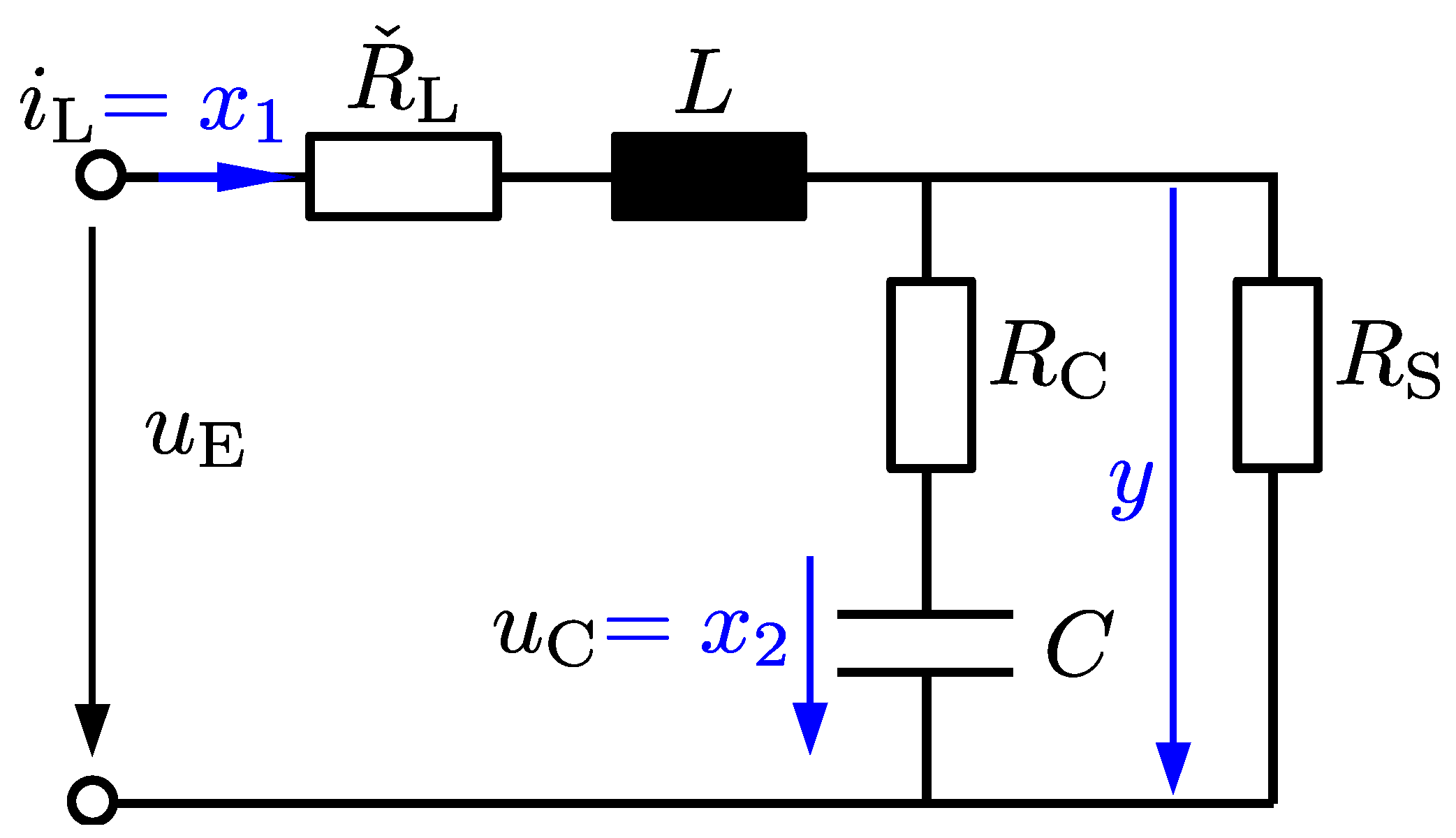
2. Modeling of an Electrical Circuit
3. Robust State-Feedback Control
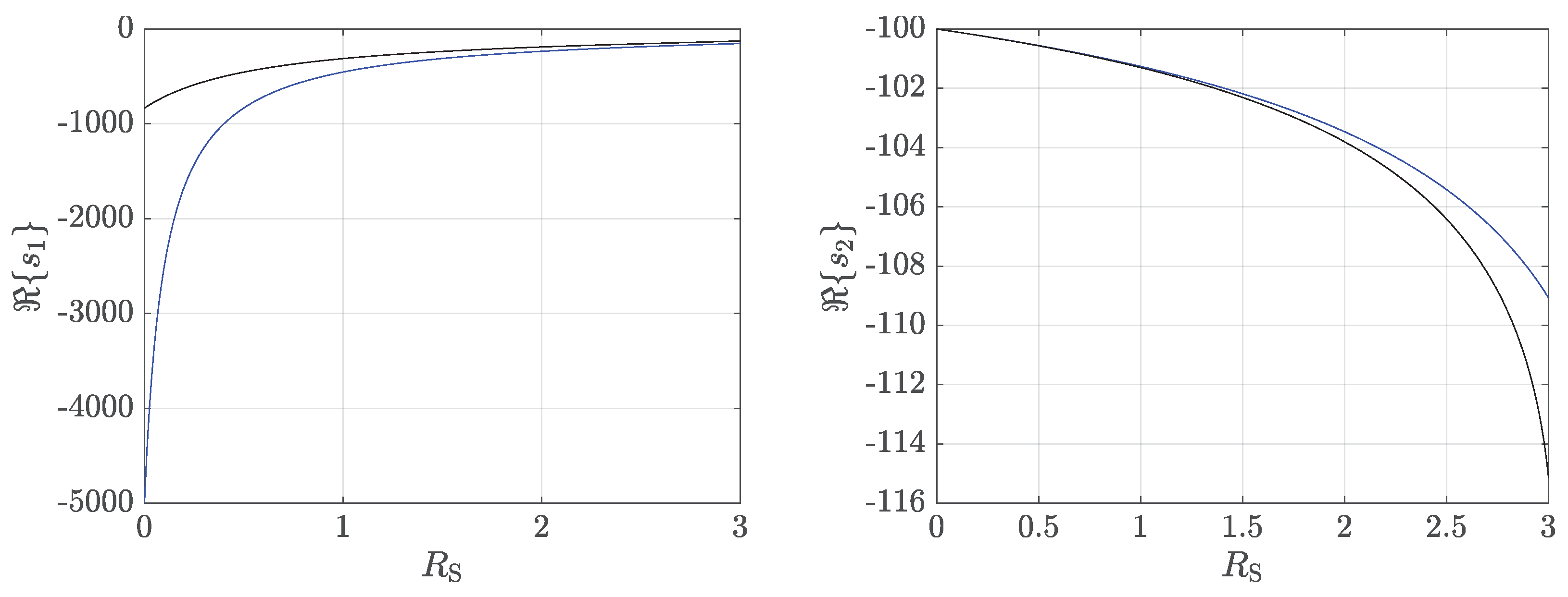
4. Transformation into a Cooperative Form
| Algorithm 1: LMI-based computation of the transformation matrix . |
 |
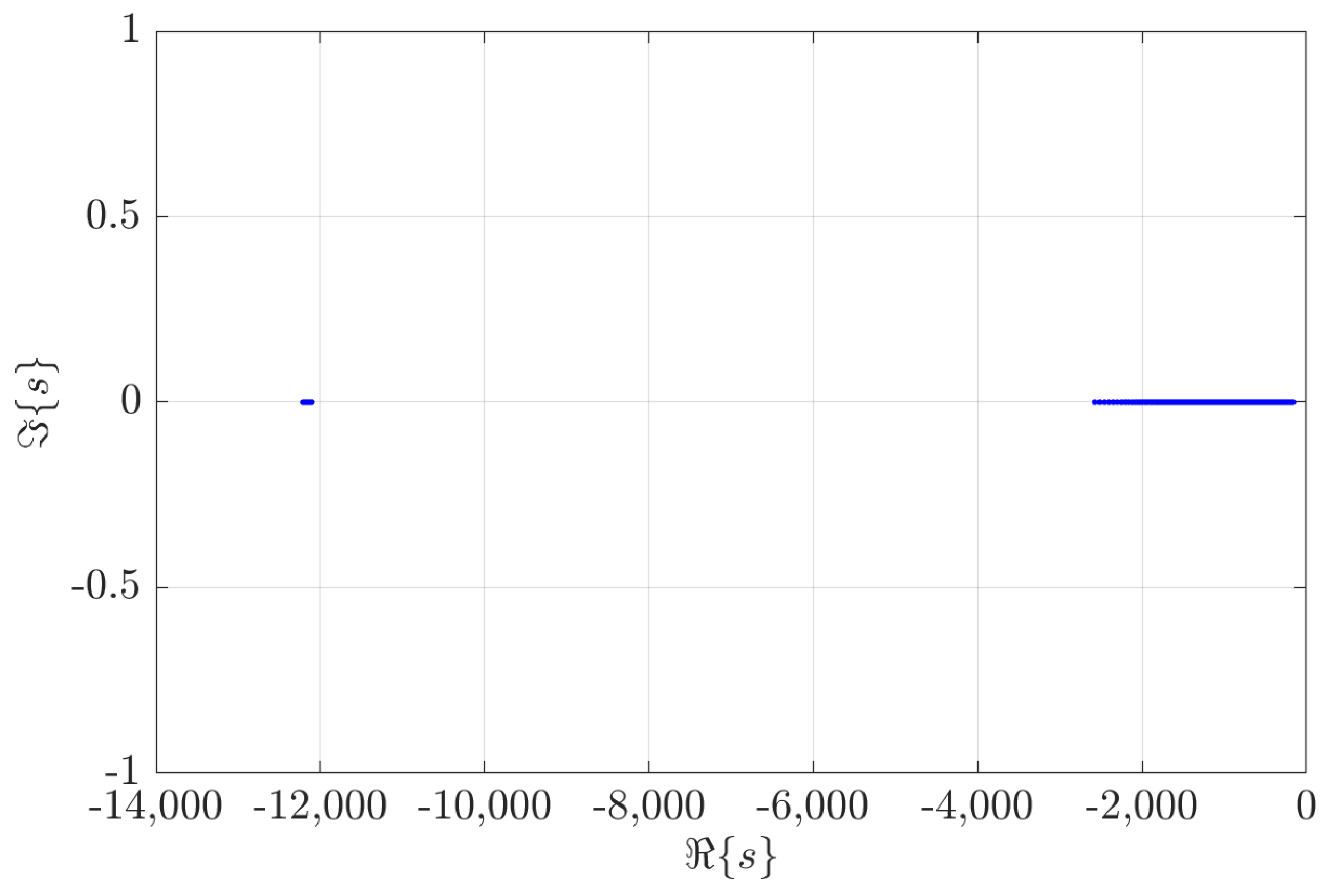
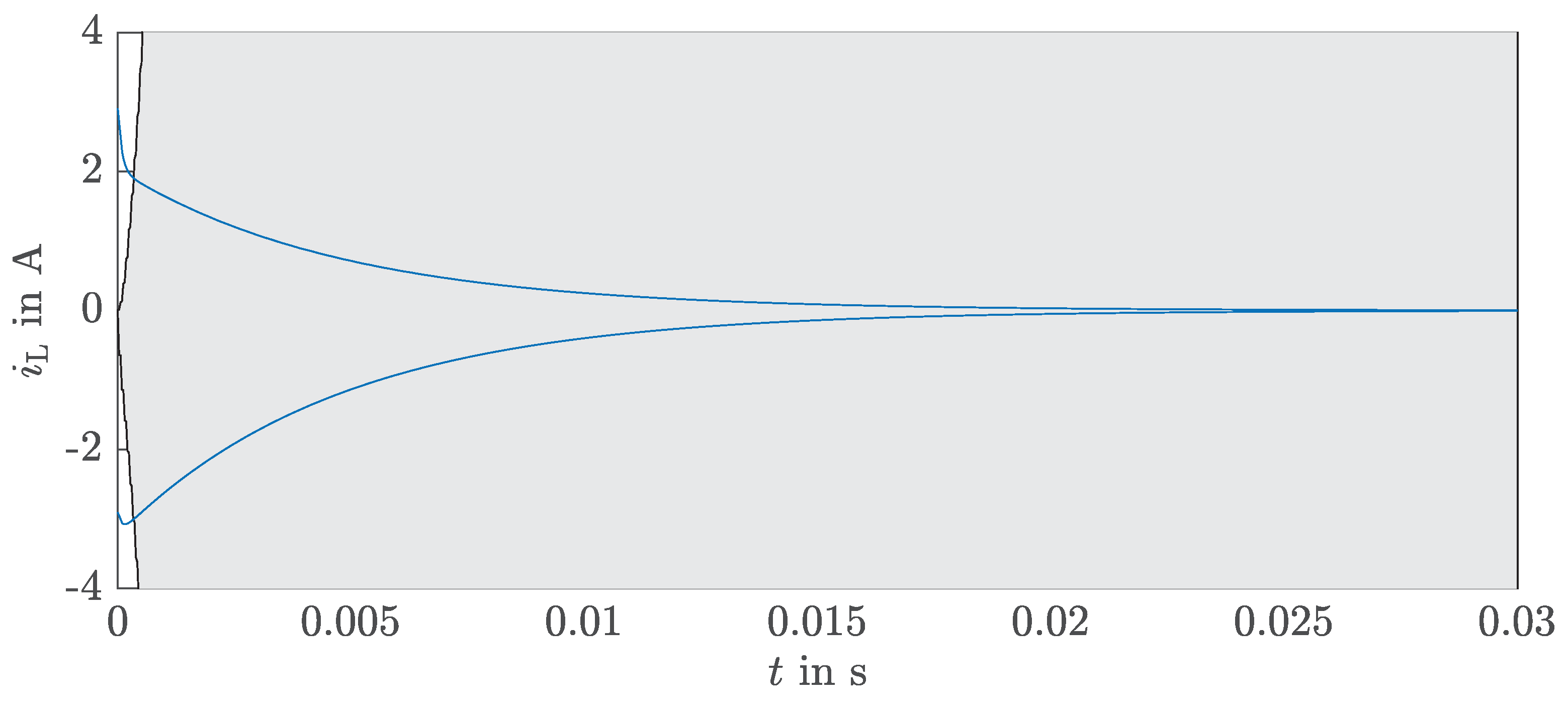
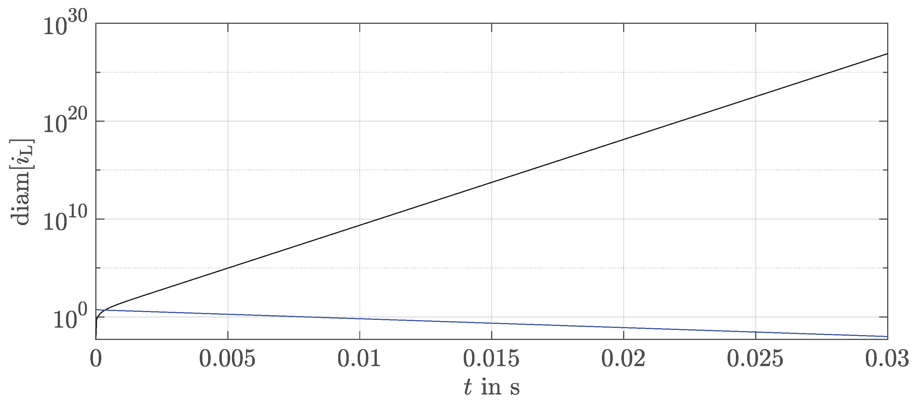
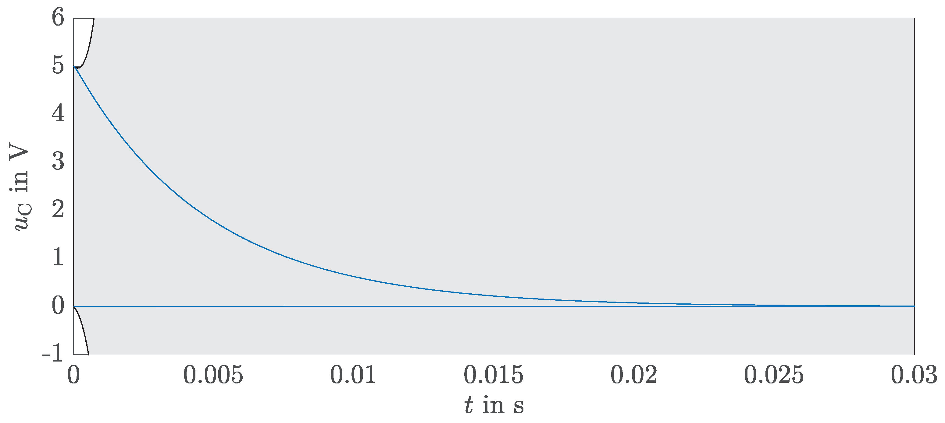
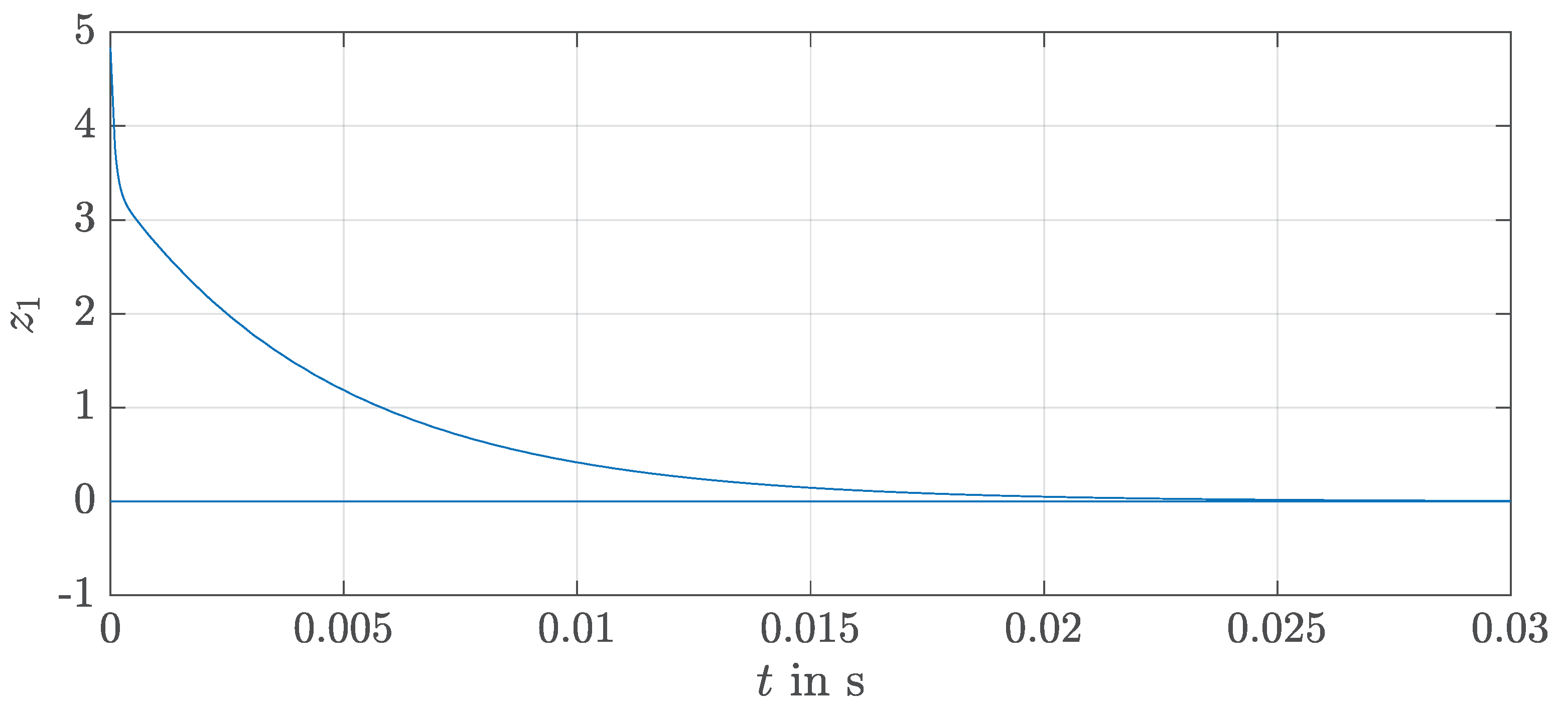
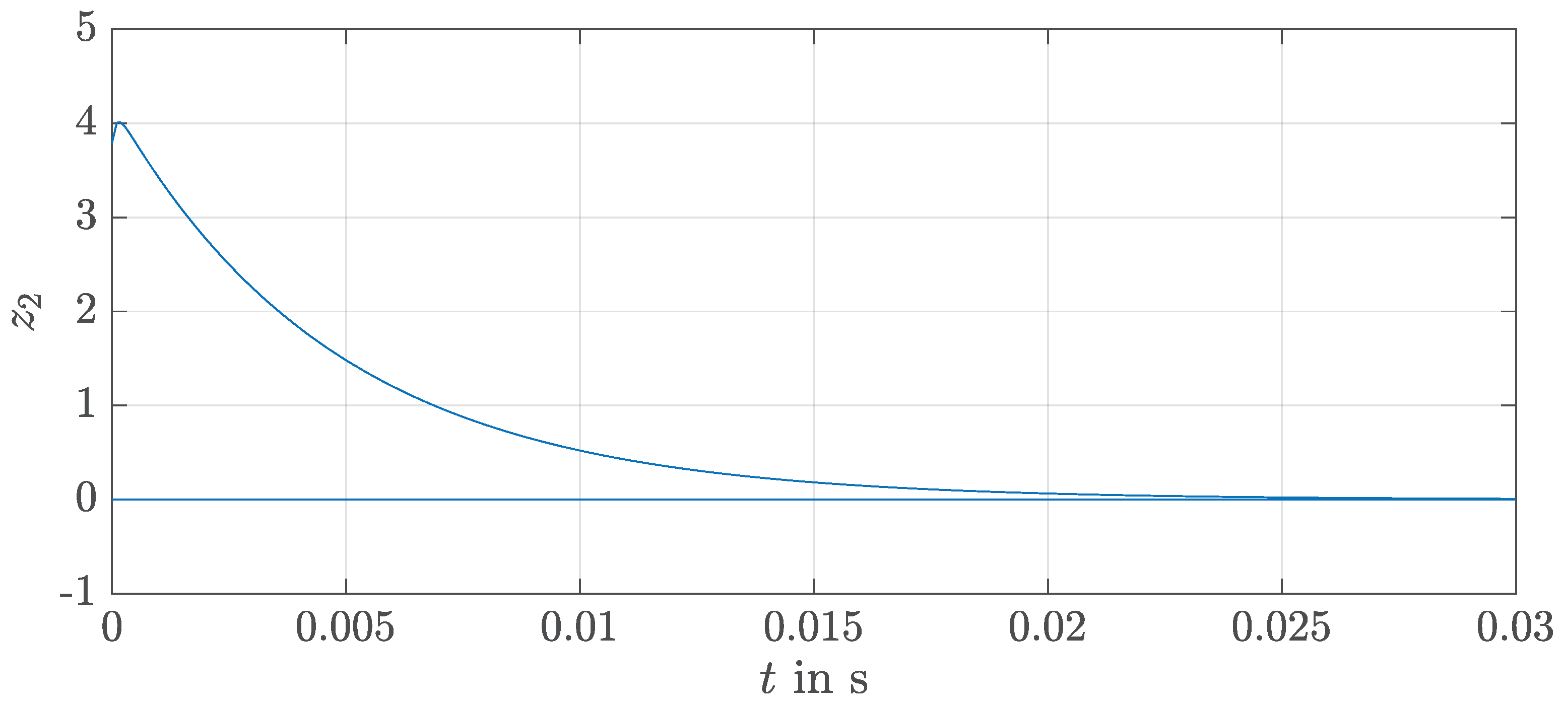
5. Simulation Results
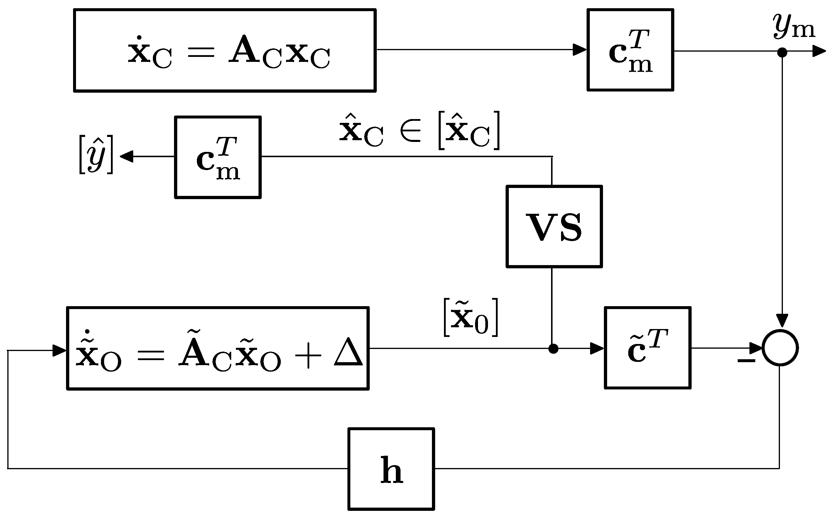
6. Observer
7. Conclusions and Future Work
Author Contributions
Funding
Conflicts of Interest
Abbreviations
| LMI | Linear matrix inequality |
| IVP | Initial value problem |
References
- Rauh, A.; Kersten, J. Transformation of Uncertain Linear Systems with Real Eigenvalues into Cooperative Form: The Case of Constant and Time-Varying Bounded Parameters. Algorithms 2021, 14, 85. [Google Scholar] [CrossRef]
- Jaulin, L.; Kieffer, M.; Didrit, O.; Walter, É. Applied Interval Analysis; Springer: London, UK, 2001. [Google Scholar]
- Nedialkov, N.; Jackson, K.; Pryce, J.D. An Effective High-Order Interval Method for Validating Existance and Uniqueness of the Solution of an IVP for an ODE. Reliab. Comput. 2001, 7, 449–465. [Google Scholar] [CrossRef]
- Nedialkov, N.S. Interval Tools for ODEs and DAEs. In Proceedings of the 12th GAMM-IMACS International Symposium on Scientific Computing, Computer Arithmetic, and Validated Numerics (SCAN 2006), Duisburg, Germany, 26–29 September 2006; IEEE Computer Society: Duisburg, Germany, 2007. [Google Scholar] [CrossRef]
- Efimov, D.; Raïssi, T.; Chebotarev, S.; Zolghadri, A. Interval State Observer for Nonlinear Time Varying Systems. Automatica 2013, 49, 200–205. [Google Scholar] [CrossRef]
- Kersten, J.; Rauh, A.; Aschemann, H. State-Space Transformations of Uncertain Systems With Purely Real and Conjugate-Complex Eigenvalues Into a Cooperative Form. In Proceedings of the 23rd International Conference on Methods and Models in Automation and Robotics, Miedzyzdroje, Poland, 27–30 August 2018. [Google Scholar] [CrossRef]
- Raïssi, T.; Efimov, D.; Zolghadri, A. Interval State Estimation for a Class of Nonlinear Systems. IEEE Trans. Autom. Control 2012, 57, 260–265. [Google Scholar] [CrossRef]
- Ifqir, S.; Rauh, A.; Kersten, J.; Ichalal, D.; Ait-Oufroukh, N.; Mammar, S. Interval Observer-Based Controller Design for Systems with State Constraints: Application to Solid Oxide Fuel Cells Stacks. In Proceedings of the 24th International Conference on Methods and Models in Automation and Robotics, Miedzyzdroje, Poland, 26–29 August 2019. [Google Scholar] [CrossRef]
- Auer, E.; Rauh, A.; Kersten, J. Experiments-based parameter identification on the GPU for cooperative systems. J. Comput. Appl. Math. 2020, 371, 112657. [Google Scholar] [CrossRef]
- Rauh, A.; Kersten, J.; Aschemann, H. Interval and Linear Matrix Inequality Techniques for Reliable Control of Linear Continuous-Time Cooperative Systems with Applications to Heat Transfer. Int. J. Control 2020, 93, 2771–2788. [Google Scholar] [CrossRef]
- Kersten, J. Cooperativity and its Use in Robust Control and State Estimation for Uncertain Dynamic Systems with Engineering Applications; Shaker-Verlag: Herzogenrath, Germany, 2020. [Google Scholar]
- Kaczorek, T. Positive 1D and 2D Systems; Springer: London, UK, 2002. [Google Scholar] [CrossRef]
- Rauh, A.; Kersten, J. From Verified Parameter Identification to the Design of Interval Observers and Cooperativity-Preserving Controllers—An Experimental Case Study. Acta Cybern. 2020, 24, 509–537. [Google Scholar] [CrossRef]
- Tietze, U.; Schenk, C. Halbleiter-Schaltungstechnik, 9th ed.; Springer: Berlin/Heidelberg, Germany, 1989. [Google Scholar] [CrossRef]
- Scherer, C.; Weiland, S. Linear Matrix Inequalities in Control. In Control System Advanced Methods, 2nd ed.; Levine, W.S., Ed.; The Electrical Engineering Handbook Series; CRC Press: Boca Raton, FL, USA, 2011; pp. 24-1–24-30. [Google Scholar] [CrossRef]
- Chilali, M.; Gahinet, P. H/sub /spl infin// Design with Pole Placement Constraints: An LMI Approach. IEEE Trans. Autom. Control 1996, 41, 358–367. [Google Scholar] [CrossRef]
- Löfberg, J. YALMIP: A Toolbox for Modeling and Optimization in MATLAB. In Proceedings of the IEEE International Symposium on Computer Aided Control Systems Design, Taipei, Taiwan, 2–4 September 2004; pp. 284–289. [Google Scholar] [CrossRef]
- Ackermann, J. Robust Control—The Parameter Space Approach; Springe: London, UK, 2002. [Google Scholar] [CrossRef]
- Sturm, J.F. Using SeDuMi 1.02, A MATLAB Toolbox for Optimization over Symmetric Cones. Optim. Methods Softw. 1999, 11–12, 625–653. [Google Scholar] [CrossRef]
- Rump, S. IntLab—INTerval LABoratory. In Developments in Reliable Computing; Csendes, T., Ed.; Kluver Academic Publishers: Dordrecht, The Netherlands, 1999; pp. 77–104. [Google Scholar] [CrossRef]
- Boyd, S.; El Ghaoui, L.; Feron, E.; Balakrishnan, V. Linear Matrix Inequalities in System and Control Theory; SIAM: Philadelphia, PA, USA, 1994. [Google Scholar] [CrossRef]
- Kersten, J.; Rauh, A.; Aschemann, H. Interval Methods for the Implementation and Verification of Robust Gain Scheduling Controllers. In Proceedings of the 22nd International Conference on Methods and Models in Automation and Robotics, Miedzyzdroje, Poland, 28–31 August 2017. [Google Scholar] [CrossRef]
- Puig, V.; Saludes, J.; Quevedo, J. Worst-Case Simulation of Discrete Linear Time-Invariant Interval Dynamic Systems. Reliab. Comput. 2003, 9, 251–290. [Google Scholar] [CrossRef]
- Rauh, A.; Kersten, J.; Aschemann, H. Linear Matrix Inequality Techniques for the Optimization of Interval Observers for Spatially Distributed Heating Systems. In Proceedings of the 23rd International Conference on Methods Models in Automation Robotics (MMAR), Miedzyzdroje, Poland, 27–30 August 2018. [Google Scholar]
- Najjar, A.; Amairi, M. Interval Observer Design for Network Controlled Systems. In Proceedings of the International Conference on Advanced Systems and Emergent Technologies, Hammamet, Tunisia, 19–22 March 2019; pp. 148–153. [Google Scholar] [CrossRef]
- Rauh, A.; Jaulin, L. Novel Techniques for a Verified Simulation of Fractional-Order Differential Equations. Fractal Fract. 2021, 5, 17. [Google Scholar] [CrossRef]
- Feng, X. Generalized Set-Theoretic Interval Observer Using Element-Wise Nonnegativity Transformation. Automatica 2020, 125. [Google Scholar] [CrossRef]


| Variable | Unit/Value | Meaning |
|---|---|---|
| L | Inductance | |
| C | Capacity | |
| Ohmic resistance of the load | ||
| Ohmic resistance of the capacity | ||
| Overall ohmic resistance of the inner resistance of the inductivity and a constant limiting resistance |
| Step | in A | in A | in V | in V |
|---|---|---|---|---|
| 1 | ||||
| 2 |
Publisher’s Note: MDPI stays neutral with regard to jurisdictional claims in published maps and institutional affiliations. |
© 2021 by the authors. Licensee MDPI, Basel, Switzerland. This article is an open access article distributed under the terms and conditions of the Creative Commons Attribution (CC BY) license (https://creativecommons.org/licenses/by/4.0/).
Share and Cite
Kersten, J.; Rauh, A.; Aschemann, H. Analyzing Uncertain Dynamical Systems after State-Space Transformations into Cooperative Form: Verification of Control and Fault Diagnosis. Axioms 2021, 10, 88. https://doi.org/10.3390/axioms10020088
Kersten J, Rauh A, Aschemann H. Analyzing Uncertain Dynamical Systems after State-Space Transformations into Cooperative Form: Verification of Control and Fault Diagnosis. Axioms. 2021; 10(2):88. https://doi.org/10.3390/axioms10020088
Chicago/Turabian StyleKersten, Julia, Andreas Rauh, and Harald Aschemann. 2021. "Analyzing Uncertain Dynamical Systems after State-Space Transformations into Cooperative Form: Verification of Control and Fault Diagnosis" Axioms 10, no. 2: 88. https://doi.org/10.3390/axioms10020088
APA StyleKersten, J., Rauh, A., & Aschemann, H. (2021). Analyzing Uncertain Dynamical Systems after State-Space Transformations into Cooperative Form: Verification of Control and Fault Diagnosis. Axioms, 10(2), 88. https://doi.org/10.3390/axioms10020088