Article

A Compensatory Fuzzy Logic Model in Technical Trading

by
Norma P. Rodríguez-Cándido
1,
Rafael A. Espin-Andrade
1,
Efrain Solares
1,* and
Witold Pedrycz
2
1
Faculty of Accounting and Management, Universidad Autónoma de Coahuila, Torreon 27000, Mexico
2
Department of Electrical and Computer Engineering, University of Alberta, Edmonton, AB T6G 2R3, Canada
*
Author to whom correspondence should be addressed.
Axioms 2021, 10(1), 36; https://doi.org/10.3390/axioms10010036
Submission received: 7 February 2021 / Revised: 4 March 2021 / Accepted: 15 March 2021 / Published: 18 March 2021
(This article belongs to the Section Logic)

Abstract

:
This work presents a novel approach to prediction of financial asset prices. Its main contribution is the combination of compensatory fuzzy logic and the classical technical analysis to build an efficient prediction model. The interpretability properties of the model allow its users to incorporate and consider virtually any set of rules from technical analysis, in addition to the investors’ knowledge related to the actual market conditions. This knowledge can be incorporated into the model in the form of subjective assessments made by investors. Such assessments can be obtained, for example, from the graphical analysis commonly performed by traders. The effectiveness of the model was assessed through its systematic application in the stock and cryptocurrency markets. From the results, we conclude that when the model shows a high degree of recommendation, the actual financial assets show high effectiveness.

1. Introduction

For many years, analysts have studied and tried to understand the movements of the market prices of financial assets, their returns, and the involved risks. In particular, the prediction of changes in the price of financial assets is a topic of substantial interest for traders, investors, and economists (simply referred to as investors in the rest of the paper) [1,2,3]. In most cases, a correct assessment of how prices will change is the determinant for the success of an investor. This is particularly pertinent when making decisions about assets that investors must buy or sell, and the right time to do so. Technical analysis is a tool widely used by practitioners that intends to meet this purpose [2,3]. Technical analysis is used to study market patterns, and demand and supply of financial assets, and consists of using price data to create rules and exploit them financially by defining the most appropriate moment to buy/sell [4]. The past two decades have seen an important increase in studies related to financial asset trading using technical analysis and, in particular, an evolution from exclusively visual analyses to more embracing and quantitative techniques. However, mathematical models for decision-making using technical analysis (MTA) remain scarce. Furthermore, the formal treatment in the literature does not aggregate technical analysis criteria for decision-making [5]. Rather, the literature approaches commonly use technical analysis to build a set of indicators related to the transaction and let the investor aggregate these pieces of information. This implies that more demanding cognitive efforts are required by the investor in comparison with approaches that aggregate the information.
Irwin and Park [6] found that 56 of 95 recent studies reported positive results from the exploitation of technical analysis but noted that many of these results were subject to doubt due to issues such as data snooping. Some academics even consider technical analysis to be a pseudoscience [7]. For example, Eugene Fama [7] states that evidence for the performance of technical analysis is sparse and inconsistent with the weak form of the efficient-market hypothesis. For the authors of the current study, the most valid criticism of technical analysis is that it is subjective [8]. As the computation technologies have emerged and improved, and larger numbers of investors have become interested in technical analysis, investors have used new heuristics that often lack a sound basis, scientific grounding, and robustness. However, the perspective of these investors is based on their own experiences and expectations; thus, they might feel misled by any MTA that does not allow their subjectivity to be incorporated. The actual requirement of MTAs is their modeling ability to interpret the investor’s tacit knowledge in a formal, reproducible way that provides recommendations on a theoretically sound basis. The principal value of this paper is the presentation of a new means of modeling the investor’s expert knowledge regarding technical analysis.
Many authors argue that technical analysis can provide useful support when identifying trends and business opportunities; these authors explain important results of technical analysis based on expert traders’ experience (see, for example, [4,9]). Moreover, the increasing interest of practitioners in using this analysis requires further and deeper assessments of its performance from the researchers’ perspective. As stated by Lo and Hasanhodzic [10], technical analysis is a legitimate and useful discipline that deserves further academic studies. Therefore, we try here to provide evidence about the performance of technical analysis in predicting the price changes of financial assets. Section 2.3 provides a description of the current research in technical analysis, in addition to the most important references in the area.
Among the different alternatives to provide an MTA with these modeling characteristics, fuzzy logic (see [11,12]) is notable due to its generality and interpretability capabilities. It is widely accepted that fuzzy logic can be applied in a range of situations such as data mining (when undertaken both supervised and non-supervised learning tasks), decision analysis, engineering, game theory, operational research, simulation, and supply chain management. The advantage of fuzzy logic regarding its interpretability capabilities refers to the plethora of tools that it can use to communicate. Natural or professional language, neural networks, fuzzy logic predicates, and graphical language (trees, graphs, maps) are commonly exploited by fuzzy logic. Zadeh [11] pioneered the theoretical background of classical fuzzy logic and his ideas are still considered as general reference points, even decades after their inception. Other very well-known theories of fuzzy logic are the Mamdani and Takagi–Sugeno (Sugeno, for brief) inference systems. The former is characterized by a simple structure of min–max operations that creates a control system by synthesizing a set of linguistic control rules obtained from experienced human operators [13]. The latter approximates actual systems by using singleton output membership functions, that is, its rule consequents are usually either numbers or linear functions of the inputs [14]. However, the non-compensatory effects and often poor interpretability of these theories may be important issues when addressing specific situations in decision making, such as ordinal classification and selection where lower truth values of a component predicate could be compensated for by high truth values of others [12]. Espín et al. [12] proved that more permissive-to-compensation approaches can be better decision-making tools regarding multiple criteria value theory. Similarly, Picos [15] found that real decision makers tend to behave in a compensatory manner.
Fuzzy sets and fuzzy logic have supported five particular approaches in modelling:
  • Semantic modelling using the opportunities associated with the approaches’ characteristics of science of vagueness, the multivalued approach, and language labels modeled by membership functions.
  • The use of expert knowledge as source for modeling, as a particular means of addressing knowledge engineering.
  • The use of different expressions of knowledge, for example, sets of rules of conditional propositions typically used to deal with fuzzy systems for automatic fuzzy control and other applications.
  • The simultaneous use of different scenarios, made possible using fuzzy sets and fuzzy logic domain.
  • The incorporation of subjective and qualitative approaches in a harmonic manner with quantitative approaches.
These approaches have been considered to be attractive, but have not been successfully used to a large extent in practice because of certain weaknesses associated with interpretability properties.
Although fuzzy logic can be compensatory in a broad sense, a new specific approach called compensatory fuzzy logic (CFL) was recently proposed in [12], whose main characteristic is satisfying a set of axioms that increase the interpretability of its methods. Section 2.2 presents an axiomatic description of compensatory fuzzy logic and argues its theoretically convenience for our purpose in this paper. CFL is a new transdisciplinary approach to address the interpretability concept and its properties, and has been used successfully in diverse problems using knowledge engineering.
This paper’s main objective is to describe a novel mathematical approach that integrates both user knowledge and literature information regarding technical analysis by exploiting compensatory fuzzy logic when trading financial assets. Therefore, the novelty of this approach lies in exploiting the CFL’s characteristics of interpretability to better represent imperfect knowledge that, plausibly, will imply a more effective trading procedure. Presenting evidence about the model’s effectiveness is also part of the paper’s main objective.
The paper is structured as follows: Section 2 offers a background to the developed work. Section 3 describes the approach proposed in this paper. Its assessment is carried out through a case study in Section 4. Section 5 offers conclusions.

2. Background

2.1. Literature Review

Investments in financial assets usually follow three main stages [16]: asset screening, capital allocation, and rebalancing. The first stage consists of assessing the often large number of assets that are available (making it possible to distinguish between “good” and “bad” assets), such that a sufficiently small subset of good assets is selected to be considered in the following stages. Capital allocation consists of defining the amounts (normally expressed as a proportion of the resources available) that will be invested in the selected assets. Finally, the rebalancing stage consists of adjusting previous conclusions to new information that will, presumably, positively impact on the overall results obtained by the investments. Technical analysis can be incorporated into any of the three phases [16,17,18]. Other typical factors used to address this type of investment, although dependent on the specific type of asset, are historical prices (time series), volume of transactions, volatility, price-to-earnings, price-to-book, price-to-sales, and price-to-cash flow [19].
A typical technique used during asset screening involves assigning a score to each asset [20,21]. The simplest technique to assign scores to assets is the weighted sum of the form ∑wiyi, where yi is the value of the ith factor and wi is its weight (e.g., [19,22,23]). The main advantage of the weighted sum is its simplicity, and its properties of transitivity, comparability, and independence with respect to irrelevant alternatives, which is convenient for creating a ranking of assets. Its main drawbacks are that it admits total compensation (it cannot consider veto effects), it requires a constant tradeoff rate (for each pair of criteria, a degraded magnitude for one of the criteria is compensated for by a fixed magnitude for which the criteria improves), it demands cardinal information in yi, and simplistic approaches might be used to determine a threshold that dictates which assets should be classified as “good”. Other common approaches followed during the asset screening phase are cluster analysis [24], linear regression [25], and approaches based on computational intelligence [16]. Regarding the latter approach, genetic algorithms [26], artificial neural networks (e.g., [27,28]), adaptive neuro-fuzzy inference systems [28], and data envelopment analysis [29,30] are used. However, with the exception of data envelopment analysis, the remaining approaches commonly used during this phase do not allow the straightforward incorporation of expert knowledge [16].
Capital allocation, often called portfolio optimization, is mainly focused on defining how much investment should be assigned to each asset selected in the first phase. This phase deals with the reduction of risk in the investment and was addressed by [31]. Markowitz stated that, for any two assets with the same expected return, the investor should select the asset with the lowest risk (considered as the statistical variability from the expected return). However, the specific proposal of Markowitz, in which the risk of an investment is given by its variance, has been strongly criticized because of a lack of pragmatism. General approaches, such as consistent risk measures with respect to stochastic dominance [32] and coherent risk measures [33,34], have been used as substitutes for classical variance as a risk measure. Of the latter, the most common are semi-variance [19,35], value at risk (VaR) [36], conditional risk value (CVaR) [37], average risk value/expected shortfall [38], and quantiles of the probability distribution [1,39]. The main difficulties with the previous risk measures are their lack of interpretability from the general perspective of investors and their high degree of dependance on historical and statistical information.
Frequent changes to supported assets, for example, in the form of allocating different investment proportions, are usually convenient to capture dynamic real-world situations. According to Andriosopoulos [16], some common approaches to rebalancing of investment in financial assets are adaptive neuro-fuzzy inference systems, artificial neural networks, genetic algorithms, and deep learning.

2.2. Compensatory Fuzzy Logic—An Outline

Vagueness and uncertainty concerning the description of the semantic meanings of statements expressed by technical analysis require specific ways of modeling. Fuzzy logic [11] has been widely accepted and used to achieve this purpose during the past five decades. Nevertheless, as stated by Espin et al. [12], some operators from classical fuzzy logic are not sensitive to changes in the truth values of the component predicates, which is a limitation when addressing problems of ordinal classification and selection because real decision makers exhibit compensatory behavior in certain situations [15]. Compensatory fuzzy logic (CFL) is a multivalued logic axiomatic approach that takes this into consideration. We now introduce the generic definitions of CFL.
Let a = ( a 1 , a 2 , , a n ) , b = ( b 1 , b 2 , , b n ) , and c = ( c 1 , c 2 , , c n ) be any three elements of the Cartesian product [ 0 , 1 ] n . Each a, b, and c might be, for example, the truth degree of a predicate of the form “it is advisable to buy financial asset x according to rule w of technical analysis”. The quartet of operators ( c , d , o , N ), where c : [ 0 , 1 ] n   [ 0 , 1 ] is the conjunction operator, d : [ 0 , 1 ] n   [ 0 , 1 ] is the disjunction operator, o : [ 0 , 1 ] n   [ 0 , 1 ] is the order operator and N : [ 0 , 1 ]   [ 0 , 1 ] is the negation operator, constitute compensatory fuzzy logic if the following group of axioms is satisfied:
I. 
Compensation Axiom
m i n ( a 1 , a 2 , , a n ) c ( a 1 , a 2 , , a n ) m a x ( a 1 , a 2 , , a n ) , and
m i n ( a 1 , a 2 , , a n ) d ( a 1 , a 2 , , a n ) m a x ( a 1 , a 2 , , a n ) .
II. 
Symmetry or Commutativity Axiom
c ( a 1 , a 2 , , a i , , a j , , a n ) = c ( a 1 , a 2 , , a j , , a i , , a n ) , and
d ( a 1 , a 2 , , a i , , a j , , a n ) = d ( a 1 , a 2 , , a j , , a i , , a n ) .
III. 
Strict Growth Axiom
If a 1 = b 1 ,   , a i 1 = b i 1 , a i + 1 = b i + 1 , , a n = b n are different to zero and a i > b i then
c ( a 1 , a 2 , , a i , , a n ) > c ( b 1 , b 2 , , b i , , b n ) , and
d ( a 1 , a 2 , , a i , , a n ) > d ( b 1 , b 2 , , b i , , b n ) .
IV. 
Veto Axiom
If a i = 0 for any i then
c ( a 1 , a 2 , , a n ) = 0 , and
If a i = 1 for any i then
d ( a 1 , a 2 , , a n ) = 1 .
V. 
Fuzzy Reciprocity Axiom
o ( a , b )   =   n [ o ( b , a ) ] .
VI. 
Fuzzy Transitivity Axiom
If o ( a , b ) 0.5 and o ( b , z ) 0.5 , then
o ( a , z ) m a x ( o ( a , b ) , o ( b , z ) ) .
VII. 
De Morgan’s Laws:
N ( c ( a 1 , a 2 , , a n ) ) =   d ( n ( a 1 ) , n ( a 2 ) , , n ( a n ) ) and
N ( d ( a 1 , a 2 , , a n ) ) =   c ( n ( a 1 ) , n ( a 2 ) , , n ( a n ) ) .
Through the fulfilment of these axioms, compensatory fuzzy logic (CFL) is interpretable according to mathematical theories and paradigms associated with social practices, notably those concerning natural and professional language, such as logic, decision-making theories and methods, and mathematical statistics. CFL can successfully address the following tasks: [40,41]
  • Evaluating the convenience of an alternative according to a predicate, obtained from expressions of the decision-maker’s preferences.
  • Searching for new convenient alternatives using the predicate.
  • Assessing the truth degree of an expression using facts and expert opinions.
  • Assessing the truth degree of an expression using facts associated with a probabilistic sample.
  • Discovering new knowledge expressed in natural language using heuristics and optimization.
  • Demonstrating and discovering new knowledge by reasoning.
A method fulfilling the described axioms is fuzzy logic based on the geometric mean. This method is compatible with many axioms of normative decision theory, and the compound predicates can be understood as utility functions [12]. Its conjunction and disjunction operators behave as multi-attribute value functions; they fulfill the strictly increasing property and the De Morgan properties, in addition to having veto capabilities [12], which is a relevant aspect of the descriptive decision theory and multicriteria decision aiding. We believe that this method can achieve our goal to effectively incorporate the investor’s knowledge in investment decisions. It has never been applied in such scenario and, in particular, in combination with technical analysis. The properties and applicability of compensatory fuzzy logic based on the geometric mean are important reasons to believe that it can be used to exploit the knowledge generated by technical analysis regarding the prediction of financial asset prices. The next sections present a brief description of this analysis and describe and assess our proposal to incorporate CFL in the prediction process.

2.3. Technical Analysis

The rules currently implemented by most of MTA according to our bibliographic study are (see [42,43]): trend lines, areas of support and resistance, moving averages, and stochastic oscillators.
Through the analysis of historical changes in the performance of financial assets, technical analysis allows the prediction of future movements of prices, which investors try to take advantage of. Nevertheless, this is far from being a trivial task, because financial asset markets are usually characterized by high complexity and non-linearity that obscure the relationships among their main components.
Technical analysis has been applied by practitioners for a number of decades (see, e.g., [44,45,46]) and numerous works claim its relevance for trading financial assets (c.f. [4,17,18]). An outstanding technique used by some of these works is regression analysis (e.g., [47,48,49]). Nevertheless, the accuracy of these approaches in practical scenarios is questionable given the high non-linearity of financial asset price changes (cf. [50]). Another outstanding technique is machine learning [51]. In the latter context, Zhang et al. [52] presented a proposal in which an auto-regressive integrated moving average and neural networks were used for time series. Huang et al. [53] used a support vector machine (SVM) to forecast the direction of financial asset markets. Banga and Brorsen [54] combined single classifier models, specifically, neural networks and logistic regression, to predict the direction of the commodity futures market using technical indicators. Nicholls et al. [55] provided evidence of the effectiveness of a co-evolved approach applying genetic algorithms. As a much lesser exploited technique, natural language processing for prediction of financial asset returns was used by Mehtab and Sen [50] in combination with machine learning, deep learning, and language processing to predict financial asset price movements. Other approaches also combine sentiment analysis to perform these types of prediction [56,57]. The common feature of these approaches is that they aim to identify patterns in financial asset price changes that can, eventually, generate profits. However, the interactions among the components and the subtleties that practitioners often express in natural language when working with technical analysis are not sufficiently modelled according to our review of the state-of-the-art research. Given the discussion of Section 2.2, we believe that compensatory fuzzy logic based on the geometric mean can be an important modelling tool in this regard. Thus, we present a detailed proposal in the next section.
An important basis of technical analysis is the Dow Theory (widely described by Rhea [58]). This theory argues that price changes for a given financial asset can be assigned to one of three classes: upwards, downwards, or horizontal movements. The jargon for the first two classes of movements identifies them as bullish and bearish, respectively. A horizontal price movement happens when both the supply and demand are almost the same, which usually occurs before the price movement continues a prior trend or reverses into a new trend. Currently, it is widely accepted that the market exhibits specific characteristics in each kind of trend; therefore, practitioners of technical analysis use tools that allow one to identify and predict the current trend. Furthermore, it is through the identification of the current trend that a specific asset is advised to be bought or sold according to the estimation of the next trend.
The principles of technical analysis derive from the observation of financial markets over hundreds of years. There are different rules in technical analysis that allow one to make an evaluation of assets; among these, we concentrate our work on the main categories of rules, namely, graphical analysis (GA), quantitative analysis (QA), and candlestick analysis (C) [59]. We now present a brief description of these categories of technical rules.
Graphical analysis studies the information provided by graphics, starting from geometric figures, mainly without the use of any additional tools. Technical rules in this category classify the “behavior of the market” in trends, technical patterns, and setbacks. The first is the general direction of the peaks and valleys in the price line of the asset. This general direction can be (i) a bullish trend, (ii) a bearish trend, or (iii) an oscillation/lateral trend. Regarding the technical patterns, two types of formations are mainly identified: change of a trend and continuation of the trend. The latter suggests that the market is “taking a breath” before continuing with the original trend. Finally, setbacks are price movements against the main trend. The original price trend changes and finds a support or resistance line.
Quantitative analysis studies a numerical series of data using mathematical and statistical indicators. It consists of applying mathematical formulas to the prices and transaction volumes of the assets with the purpose of facilitating investment decision-making and predicting future prices in specific situations. The advantage of this analysis compared to the previous graphical analysis is the reduction of subjectivity. Technical rules of quantitative analysis are divided into two categories: moving averages and oscillators. Moving averages are the most versatile and spread technical indicators; they can be easily quantified. The most common moving averages are simple moving averages, Bollinger bands, and weighted moving averages. Oscillators are mathematical models applied to the price behavior. The most common oscillators are the moving average convergence/divergence and the stochastic oscillator.
By comparison, an interesting characteristic of candlesticks is that they allow one to efficiently analyze the opening, closing, highest, lowest, and overall range of prices of an asset in a given period [60]. A candlestick pattern is a sequence of candlesticks on a candlestick chart, which is mainly used to identify trends.
In this work, we assume that the investor can use and interpret a set of rules from technical analysis and that he/she is willing to provide a truth degree of a financial asset fulfilling each of these rules. Assigning truth values to agreement of the market situation with certain technical rules is straightforward; it does not require a cognitive effort other than that already required in the common practices of the investor. This is because, to exploit technical analysis (even without the proposed approach), practitioners must assess the current situation of the market and specify the extent to which the technical rules are fulfilled. The difficulty of using the proposed approach is not significant because its user is only required to express this extent of fulfillment as a truth degree. This degree is provided to the proposed approach as an input.
Numerous rules are widely applied by practitioners of this kind of approach, but it is outside the scope of this paper to provide a description of how they work. The reader is referred to [1] for algebraic definitions, [17] for graphical definitions, and [4,18] to explore case studies where this type of analysis is performed.

3. Compensatory Fuzzy Logic Model for Trading Based on Technical Analysis

Here, we present a novel MTA that uses a set of rules to decide what and when to buy and/or sell financial assets according to user knowledge and exploiting compensatory fuzzy logic based on the geometric mean.
Some information useful for decision-making in the financial asset market is the following:
  • A financial asset is good for the portfolio if it has presented high volume and high volatility systematically during a long period of time.
  • An asset should be bought (long position) at moment t if all valid rules of technical analysis for the bullish trend or oscillation are satisfied and all the general indicators are in favor of that operation.
  • An asset should be sold (short position) at moment t if all valid rules of technical analysis for the bearish trend or oscillation are satisfied and all the general indicators are in favor of that operation.
A plausible manner of exploiting the previous knowledge to select the financial assets that will compose the investment portfolio is as follows. First, identify the financial assets that are good, in the sense related to Statement 1. Second, from these good financial assets, select those whose convenience of buying or selling is greater than a “sufficiently high” degree (according to (i) state-of-the-art literature, (ii) expert recommendations, and, above all, (iii) preliminary experimentations, we concluded that the most convenient value for such a degree is 0.8). Finally, define the proportion of resources to be invested in each selected financial asset proportional to the truth value of its buying or selling convenience, and its volatility. Now we present our proposed approach to build a financial asset portfolio specifying the buying or selling contexts in the following two subsections.

3.1. Buying Model

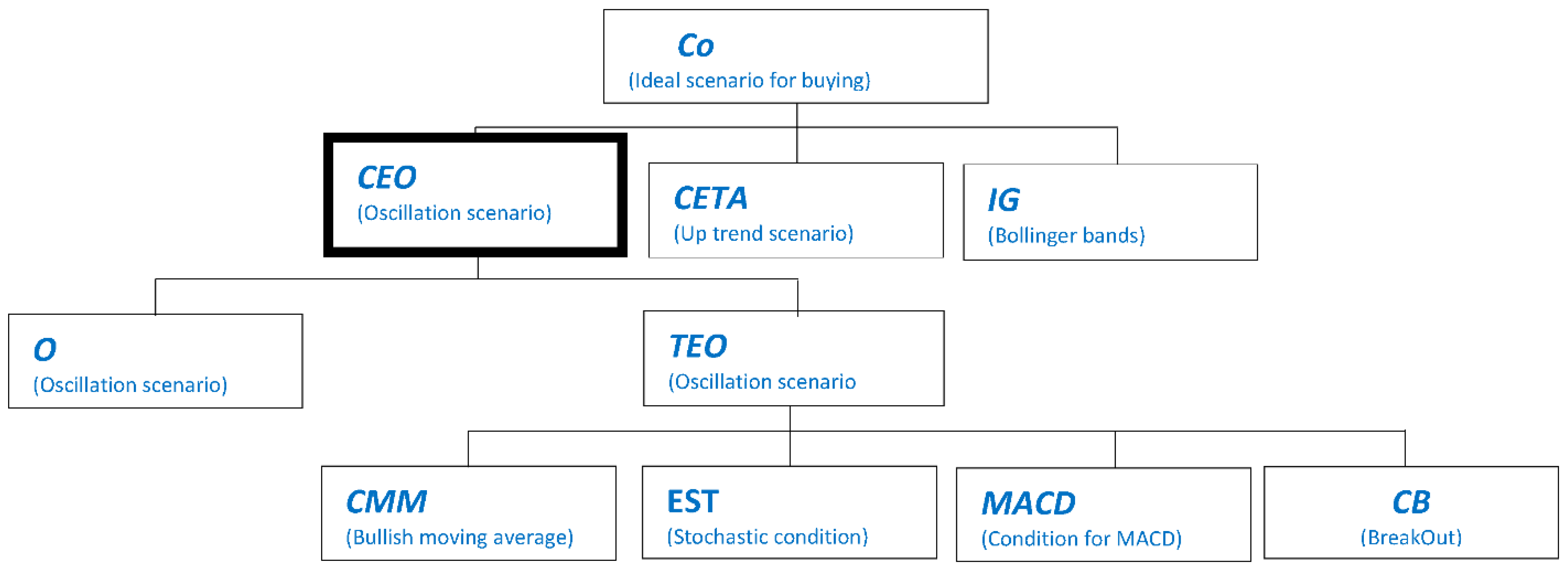
We now introduce and define the structure of our buying model. We define this model assuming that an asset should be bought in time t when it is sufficiently true that “the asset is ‘good to be bought’ at time t”. We denote the truth degree of this assertion as Co(t). We believe that the assertion should be built on the basis of three simpler assertions; that is, “the asset is ‘good to be bought’ at time t if and only if it is true that there are good oscillation conditions at time t and it is true that there is a bullish scenario in time t and it is true that Bollinger bands indicate that the financial asset should be bought in time t”. Therefore, if CEO(t), CETA(t), and IG(t) are the truth values of the three components, respectively, then:
CO(t) = CEO(t) ∧ CETA(t) ∧ IG(t),
where ∧ is the conjunction operator defined in Section 2.2 (here and in the following subsections, for readability purposes, we use a slightly different notation with respect to that used in Section 2.2); see Figure 1.
In the proposed approach, the truth degree of the “good oscillation conditions” scenario at moment t is a thesis defined as “if there is oscillation at time t then the conjunction of four assertions is true”. Thus, “it is true that there are good oscillation conditions at time t if and only if it is true that the rule associated with moving averages indicate so and it is true that the set of rules associated with stochastic oscillators indicate so and it is true that the set of rules associated with the moving averages of convergence/divergence indicate so and it is true that it is true that there is a situation of a break out”. Let O(t) denote that time t belongs to an oscillation scenario, that CMM(t), EST(t), MACD(t), and CB(t) denote the truth degrees of the four assertions, respectively, and TEO(t) denotes the conjunction of these assertions. Then, the truth degree of CEO(t) is given by:
CEO(t) = O(t) ⇒ TEO(t) = (CMM(t) ∧ EST(t) ∧ MACD(t) ∧ CB(t)).
where ⇒ denotes implication. See Figure 2.
Similarly, if TA(t) indicates that time t is part of a bullish situation and TETA(t) is a conjunction of other three predicates R(t), FB(t), and CDMM(t), where R(t) is the graphic of price returns to a line of tendency or to a moving average, FB(t) means that there is a bullish candle sheet formation in t, and CDMM(t) is the truth degree of a moving average crossing the price graphics close to t, then:
CETA(t) = TA(t) ⇒ TETA(t) = (R(t) ∧ FB(t) ∧ CDMM(t)).
Each of the truth degrees in the conjunction of the right side of the implications is formed by the truth degrees assigned by the investor to a set of rules, or new composed predicates. In the experiments shown in Section 4, we assume that the set of rules and composed predicates for the buying model are formed as shown in Figure A1 and Figure A2 of Appendix A; the notation used in these figures is described in Table A1 of Appendix C.

3.2. Selling Model

We define the truth degree of the assertion “it is true that the asset should be sold at time t”, V(t), as a conjunction of the three predicates:
  • CEO(t): The conditional associated with the scenario of oscillation at moment t is satisfied.
  • CETB(t): The conditional associated with the bearish scenario at moment t is satisfied.
  • IG(t): Conditions associated with general indicators such as Bollinger bands are satisfied.
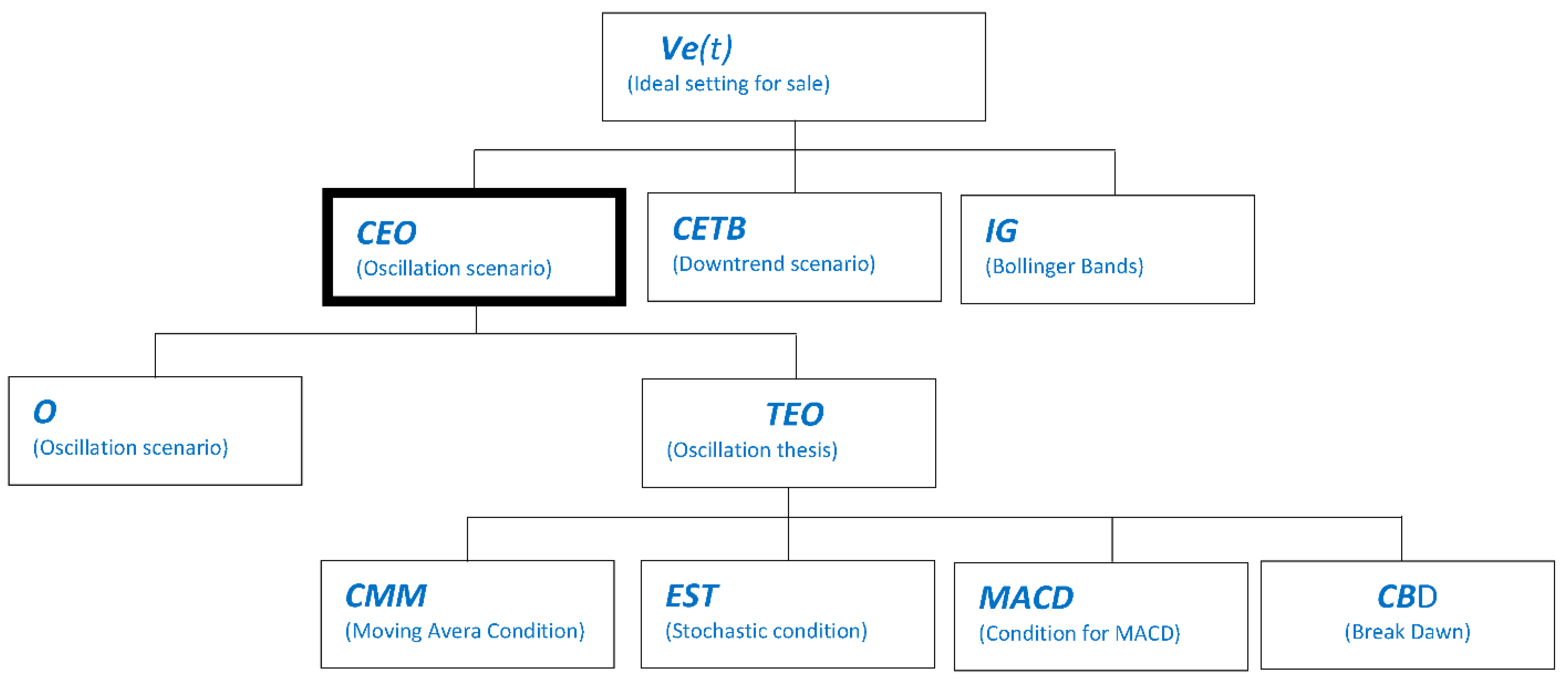
CEO(t) for the buying model is thus defined as (see Figure 5):
CEO(t) = O(t) ⇒ TEO(t).
where O(t) is the truth degree of time t belonging to a scenario of oscillation. TEO(t) is a conjunction of other four conditions:
  • CMM(t): moving average condition,
  • EST(t): Stochastic oscillator condition
  • MACD(t): Moving Average Convergence Divergence (MACD)condition
  • CBD(t): moving average condition for clear situation of break down
Therefore:
TEO(t) = (CMM(t) ∧ MACD(t) ∧ CBD(t)) is represented by the logical tree of Figure A3 of Appendix B.
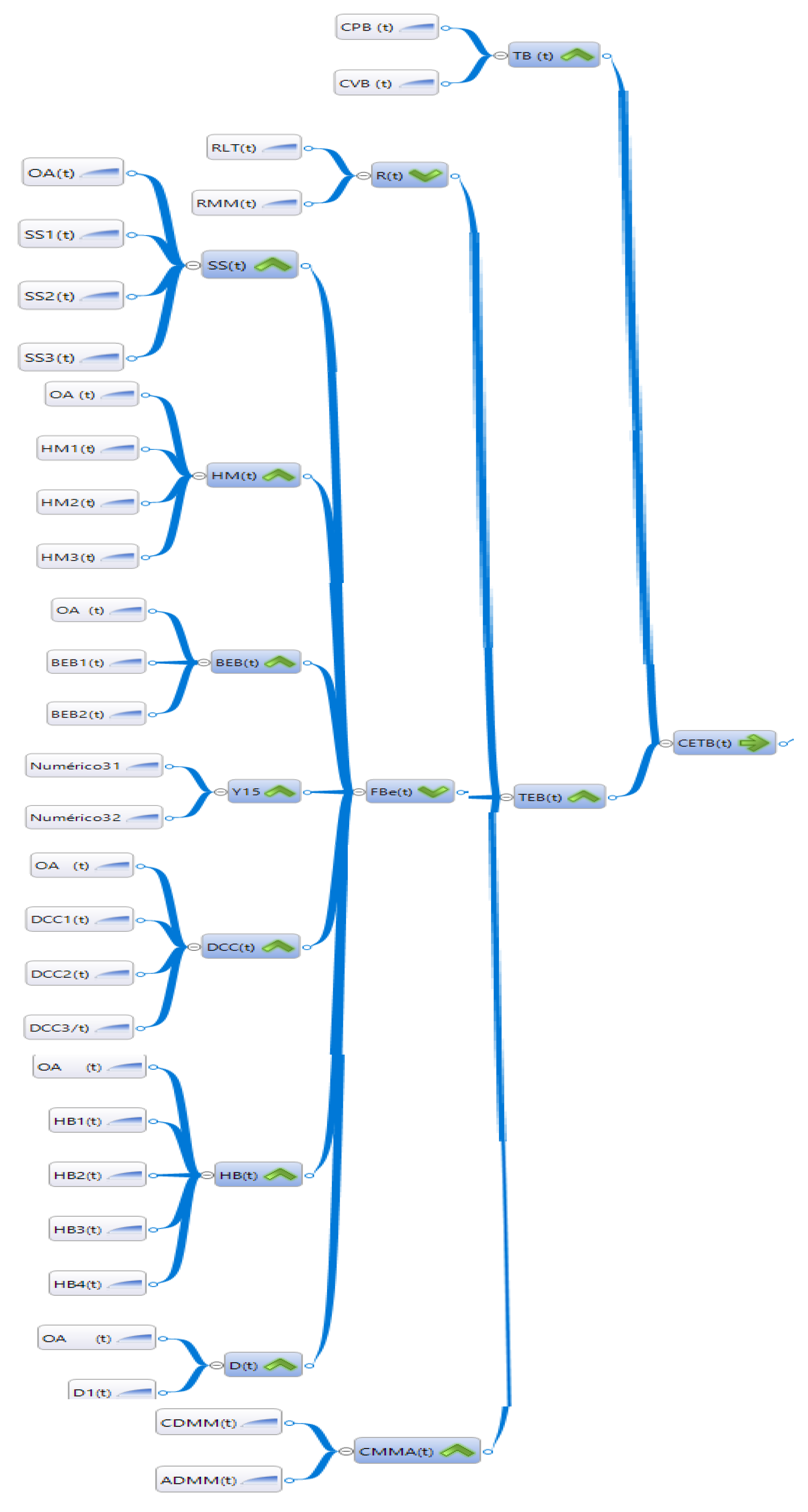
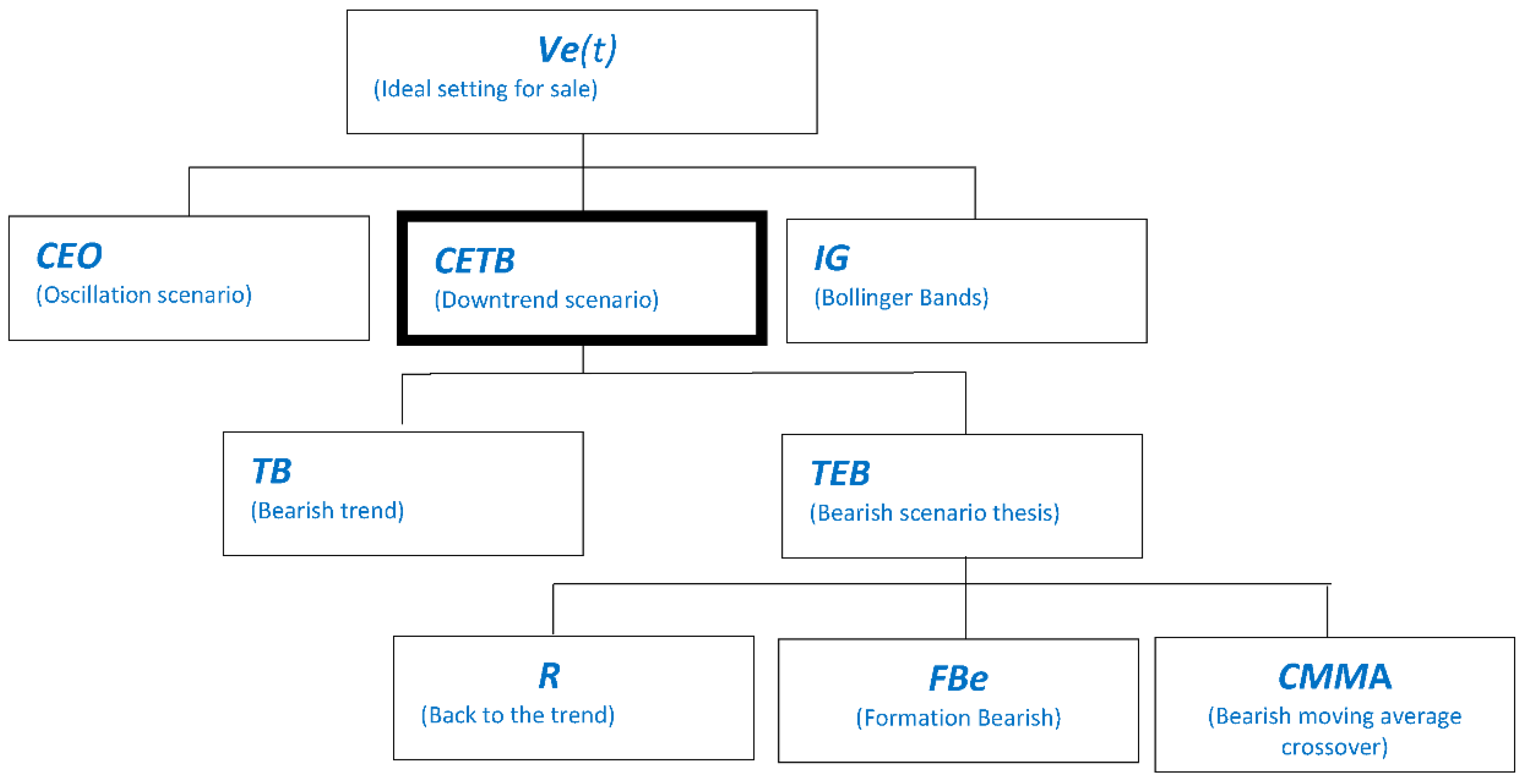
Furthermore, CETB(t) is defined as (see Figure 6):
CETB(t) = TB(t) ⇒ TEB(t).
where TB(t) indicates that time t is part of a bearish scenario and TEB(t) is a conjunction of other three predicates:
  • R(t): The graphic of price returns to a line of tendency or to a moving average
  • FBE(t): There is a bearish candle sheet formation in time t
CMMA(t): moving average crosses the price graphics close to time t.
Thus:
TEB(t) = (R(t) ∧ FBE(t) ∧ CMMA(t)).
In the experiments of Section 4, we assume that the set of rules and composed predicates for the selling model are represented by the logical tree as illustrated in Figure A3 and Figure A4 of Appendix B; the notation used in these figures is described in Table A2 of Appendix C.

3.3. Overall Procedure

Further decision-making problems related to buying and/or selling financial assets are stated as follows: (i) from a plethora of financial assets, choose those that are “convenient to invest in general”; (ii) from the assets chosen in (i), identify those that are “convenient for buying at moment t”; (iii) from the assets chosen in (i), identify those that are “convenient for selling at moment t”; and, (iv) determine the proportions of resources to be invested in each of the assets that will be bought/sold. Plausible procedures to address the four problems are the following:
Problem (i):
  • From a set of pre-screened assets, calculate the truth value of the predicate G(a, t) that models the expression “asset a is good for the portfolio according to the available information during time t”.
  • If G(a, t) is greater than a predefined value greater than 0.5, then asset a is incorporated to the set of “good” assets.
Problem (ii):
  • Calculate, for each asset in the set of “good” assets, the value of the predicate Co(t) (see Equation (1)).
  • If Co(t) for asset a is greater than a predefined value greater than 0.5, then a is incorporated to the set of assets convenient for buying at moment t.
Problem (iii):
  • Calculate, for each asset in the set of “good” assets, the value of the predicate V(t) (see Equations (4) and (5)).
  • If V(t) for asset a is greater than a predefined value greater than 0.5, then a is incorporated in the set of assets convenient for selling at moment t.
Problem (iv):
There are two scenarios where asset a will be supported with a given amount, depending on a being in or a being in .
-
If a belongs to (a has been determined as suitable for buying), determine the amount to be invested in asset a as the percentage of resources equivalent to the proportion with which a belongs to regarding the sum of the truth degrees with which the rest of assets in belong to .
-
If a belongs to (a has been determined as suitable for selling), determine the amount to be invested in asset a as the percentage of resources equivalent to the proportion with which a belongs to regarding the sum of the truth degrees with which the rest of assets in belong to .
Note that, in general, the predefined values used as thresholds in the procedures described for Problems (i)–(iii) can be elicited directly or indirectly. That is, the investor can directly provide such values, or an interactive–constructive approach can be followed; in the latter, for example, the investor provides some reference decisions and the approach finds the values that best suit those decisions.
The notion of the procedure described for Problem (iv) is related to the ordinal characteristic shown by the estimated truth values. Following this ordinal characteristic, we can ensure that the higher the truth value of buying or selling for asset a regarding the rest of assets, the higher the proportion of resources that should be invested in asset a.

4. An Illustrative Case Study: An Analysis of the Cryptocurrency Market

Our model was applied and assessed in the contemporary relevant contexts of stock and cryptocurrency trading.
The main characteristic of cryptocurrencies, a type of digital currency, is that cryptography is used to confirm transactions. Using cryptocurrency mining, users can exploit computational power to solve mathematical problems that would allow participants of the cryptocurrency market to perform new transactions; this is a common way in which new cryptocurrency units are put into operation (they are awarded to those users that solve the mathematical problems). According to [61], a cryptocurrency is a system fulfilling the following characteristics:
  • The system does not require a central authority.
  • The system keeps an overview of cryptocurrency units and their ownership.
  • The system defines whether new cryptocurrency units can be created. If new cryptocurrency units can be created, the system defines the circumstances of their origin and how to determine the ownership of these new units.
  • Ownership of cryptocurrency units can be proved exclusively cryptographically.
  • The system allows transactions to be performed in which ownership of the cryptographic units is changed. A transaction statement can only be issued by an entity proving the current ownership of these units.
  • If two different instructions for changing the ownership of the same cryptographic units are simultaneously entered, the system performs at most one of them.
The boom of cryptocurrencies in the past decade is due to the interesting properties they achieved in early 2009 due to the publication of [61,62]:
Limited anonymity—When following rules (see [63]) traders cannot be easily identified.
Independence from central authority—Decentralization reduces the probability of a single point of failure, provides the ability that the consensus rules can only be achieved by consensus of the majority, offers less censorship, and ensures that cryptocurrencies cannot be abolished but will only cease to exist when users no longer use them.
Double spending attack protection—A single cryptocurrency cannot be given to more than one recipient. For digital currencies this is a crucial and difficult problem to address, particularly in the presence of a decentralized cryptocurrency.
Aiming to apply and assess our proposal in the context of cryptocurrency trading, we exploited the well-known platform “Etoro”. This assessment was performed for both buying and selling operations.

4.1. Experimental Procedure

To assess our proposal, we exploited both the buying and selling models by evaluating a set of financial assets and investing in them according to the results of the models.
The experimental procedure used in this work consists of three stages: (i) a prescreening phase where a set of assets is selected using a given heuristic; in our experimentation, we selected those assets that were currently traded by specific well-known investors; (ii) application of the buying model and selling model on the set of selected assets; and (iii) assessment of the results.
To provide sufficiently large samples, we required that the first stage should select 17 stocks and 17 cryptocurrencies. Thus, each instance of our experiments dealt with a dataset of 34 elements. We implemented 62 instances, assessing a total of more than two thousand assets. In the second stage and for each instance, our models recommend if each asset should be (i) bought, (ii) sold, or (iii) discarded to build our portfolio of supported assets. Finally, in the third stage of the experiments, we determine (i) for each instance and for each asset, if the recommendation provided by the models achieved a positive or a negative return, and (ii) the overall effectiveness of our approach regarding the type of operation and the truth degree used as a “cutting threshold” to perform these operations. This cutting threshold allowed us to determine if a given asset should be supported.

4.2. Results

Table 1 provides a simple example of the results obtained. This table shows: (i) the date when the analysis and assessment of assets was performed for the corresponding instance; (ii) the name of the asset; (iii) if the operation performed was buying (long position) or selling (short position); (iv) the truth value of the operation as defined by the approach; (v) the result of the operation specifying if the return was positive or negative; (vi) the price of the asset when the operation was performed; (vii) the price of the asset when the operation was closed; (viii) the return obtained by the operation; and (ix) the number of days that the operation was active.
The goal of the experiments was to determine the effectiveness of the proposed approach. This effectiveness is defined here as a function of the results obtained when performing transactions. In particular, for each transaction performed in the experiments, we determined if the outcome of the investment was positive or negative. Take, for example, the first instance of Table 1. On 13 July, the model proposed to short-sell Zcash (that is, the model determined that its price would probably go down); Zcash is a cryptocurrency that uses cryptography to provide an advanced method of privacy. The truth value found by the model to provide this recommendation was 1. Because the price of the opening position was $60.07 and its closing price was $60.05, then the outcome of this particular transaction was positive. If the investor had carried out such an operation in practice, he/she should have obtained a return that would have increased his/her total earnings (ignoring expenses such as taxes and transaction costs). Finally, the positive outcome was reached after three days.
Only the results for eleven instances are shown in Table 1. We determined that only those operations with a truth degree of at least 0.8 should be supported. This was determined, as described above, due to different reasons, where the results of preliminary experiments were outlined. Of the 374 assets assessed in the instances of Table 1, our approach advised to support only 33. Notable, it advised to not support any asset on July 15th. This behavior is representative of our population of experiments: of the more than two thousand assets assessed during our experiment, the proposed approach advised to support only 278 and there were 10 days where the approach concluded that it was better not to support any asset.
The most notable conclusions that were generated from the population of experiments is that the proposed approach generated positive returns in more than 93 percent of the operations performed. This can be clearly seen in Table 1, but it can also be seen in the actual results of the population of experiments. The table of these results is easily accessible through the following link: https://bit.ly/3aO85U9 (accessed on 23, February 2021).
Table 2 presents the effectiveness of the proposed approach regarding given thresholds. This table shows the number of assets that both the buying and selling operations were advised to trade with respect to different thresholds of truth values. This indicates, for example, that of the more than two thousand assets presented to the buying model, only five were advised to be bought with a truth degree of 1.0. When we bought them during the experiment, they all generated profits. However, of the 57 assets that were advised to be sold with a 1.0 truth value, only 53 (93%) generated profits.
These results provide evidence that our proposals in this work are highly effective, particularly when these proposals create recommendations with high truth degrees.

5. Conclusions

This paper presents a novel model to trade financial assets. Its main contribution to the related literature is the exploitation of the so-called compensatory fuzzy logic based on the geometric mean method in the context of stock and cryptocurrency markets. This method fulfills an important axiom regarding the representation of knowledge. Our approach is able to (i) consider the investors’ opinions expressed in natural language and (ii) construct a logical model to define the truth degree about the buying (long position) or selling (short position) convenience of a given asset. Furthermore, our model can address numerous rules of so-called technical analysis that allows it to incorporate information about different scenarios during the assessment of assets. Thus, the proposed model can provide the investor with plausible arguments about the appropriateness of each asset that eventually leads to the construction of his/her investment portfolio.
We extensively assessed our model’s performance and effectiveness in several case studies related to stock and cryptocurrency trading. The results shown in Table 1 and Table 2 show that the model is able to identify those assets with a high truth degree of buying or selling convenience that were, in most cases, represented in portfolios that generated profits. In particular, Table 2 shows an evident tendency to reduce the absolute number of negative results as the truth degree used as a cutting threshold was increased to believe the assertion “the asset is advised to be bought/sold”.
Currently, the research requires more data to prove the effectiveness of the model. However, this work demonstrated an essential advance in mathematical modeling by implementing technical analysis.
Investigations and future work should include aspects not addressed in this work. The most relevant of these are:
  • Elaboration and application of exhaustive experiments.
  • Improvement of the model with the applications of new rules and models of technical analysis.
  • Compatibility with human behavior.
  • Compatibility with different platforms.

Author Contributions

Conceptualization, N.P.R.-C. and R.A.E.-A.; Data curation, N.P.R.-C. and R.A.E.-A.; Formal analysis, E.S.; Methodology, N.P.R.-C. and R.A.E.-A.; Project administration, R.A.E.-A.; Resources, N.P.R.-C.; Software, N.P.R.-C.; Validation, E.S. and W.P.; Visualization, W.P.; Writing—original draft, N.P.R.-C.; Writing—review & editing, E.S. and W.P. All authors have read and agreed to the published version of the manuscript.

Funding

This research received no external funding.

Institutional Review Board Statement

Not applicable.

Informed Consent Statement

Not applicable.

Data Availability Statement

Conflicts of Interest

The authors declare no conflict of interest.

Appendix A. Logical Trees of a Buying Model
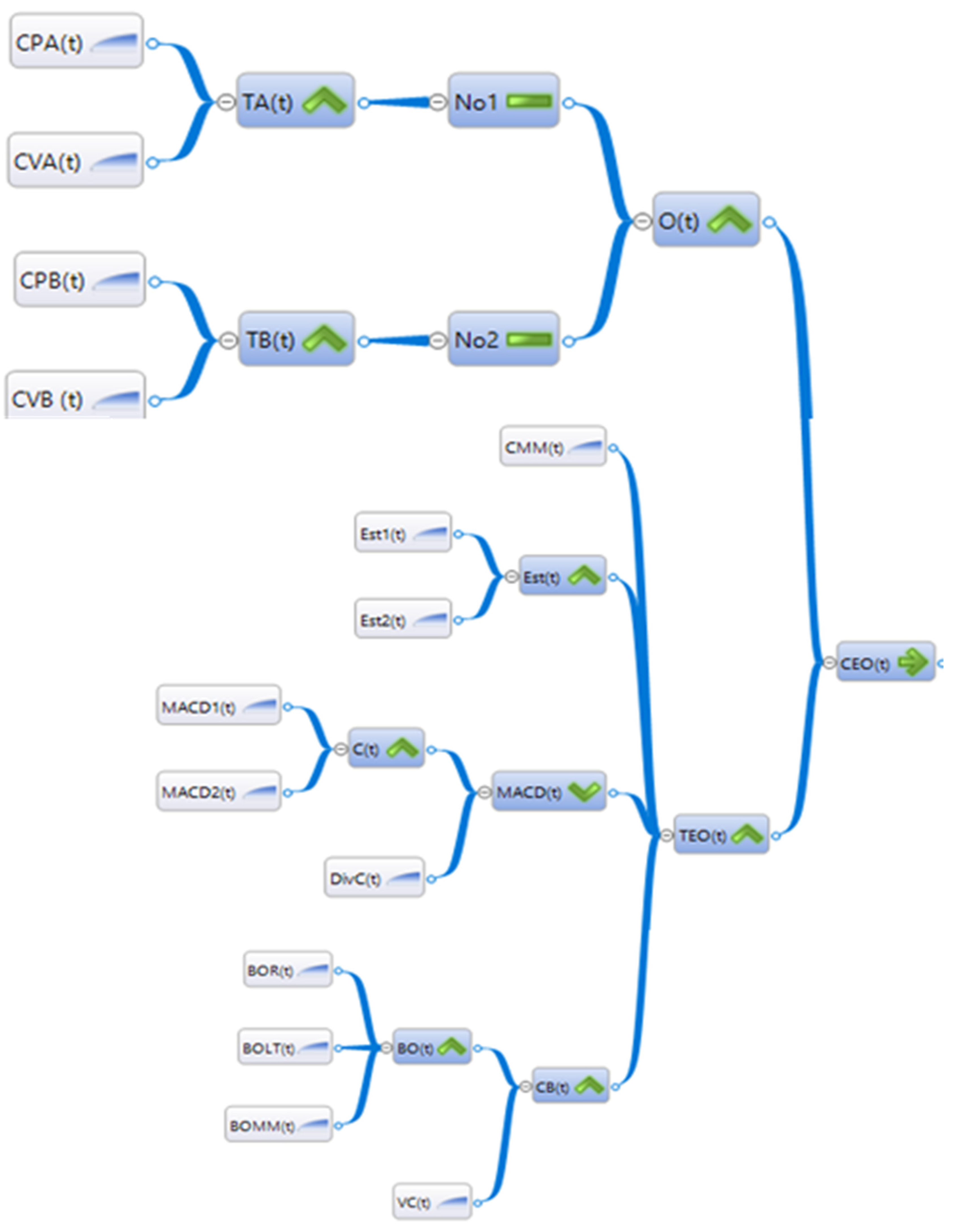
Figure A1. Logical tree representing the truth degree of the predicate “there are good oscillation conditions for buying at time t”, CEO(t).
Axioms 10 00036 g0a1
Figure A2. Logical tree representing the truth degree of the composed predicate “there is a bullish scenario at time t”, CETA(t).
Axioms 10 00036 g0a2

Appendix B. Logical Trees of a Selling Model
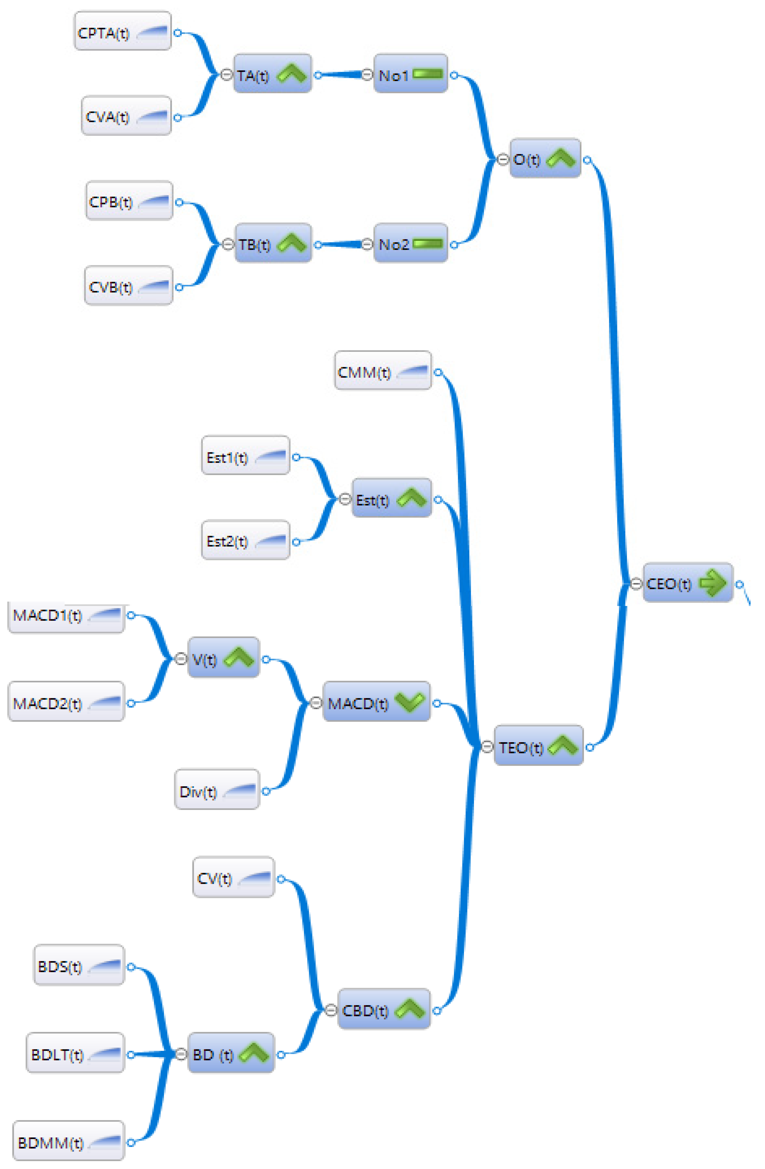
Figure A3. Logical tree representing the truth degree of the composed predicate “there are good oscillation conditions for selling at time t”, CEO(t).
Axioms 10 00036 g0a3
Figure A4. Logical tree representing the truth degree of the composed predicate “there is a bearish scenario at time t”, CETB(t).
Axioms 10 00036 g0a4

Appendix C. Definitions and Notation Used by the Proposed Models

Table A1. Notation used in the buying model.
RulePredicateKnowledge Expressed by the PredicateCategory
Trend (T)TABullish trendGA
TBBearish trendGA
OBPart of a bearish trend.GA
OOscillation trend.GA
CPAPeaks going upGA
CVAValleys going upGA
CPBPeaks going downGA
CVBValleys going downGA
Moving Averages (CMM)CMMThe fast moving average goes through the slow moving average from up to down.QA
Stochastic (Est)EST1The percent “K” goes through the stochastic moving average from up to down.QA
EST2Stochastic and moving are above of the line “80”.QA
MACDMACD1MACD crosses the signal line from top to bottomQA
(MACD)MACD2MACD and signal line are above of the line “0”QA
Divergence (DIV)DIVThe prices grow but macd’s histography is decreasing.QA
Breakdown (BD)BDSThere is a breakdown of a supportGA
BDLTExists a breakdown of a trend line of the actual wave.GA
BDMMThere is a breakdown of the moving averageGA
Volume (CV)CVThere is a significant increase in volumeQA
Trend line (R)RLTPrice returns to trend lineGA
RLMPrice returns to the moving averageGA
Shooting Star (SS)SS1The upper tail is at least twice as long as the bodyC
SS2The body is at the bottom of the candleC
SS3The lower tail is absent or too smallC
The Hanging Man (HM)HM1The lower tail is twice as long as the bodyC
HM2The body is on topC
HM3The upper tail almost does not existC
Bearish Engulfing Bar (BEB)BEB1The first candle is short and greenC
BEB2The second candle is red and wraps the previous candleC
Doji (D)DClosing and opening prices are very closeC
Dark Cloud Cover (DCC)DCC1The first candle is long and green, it is above the trend lineC
DCC2The second opens above the maximum of the previous candle and is redC
DCC3The second candle closes below half of the previous green candle
Harammi Bearish (HB)HB1There is a long green candleC
HB2It is followed by a red candle that opens below the closing of the previous red candleC
HB3The mentioned red candle is wrapped by the previous green candleC
HB4There is another red candle after the previous oneC
Moving Average (CMMA)CEMMShortly before “t” the price closes below the moving averageQA
AEMMIn the following period the price opens below the moving averageQA
Bollinger Bands (IG)BBPrice is too close or crosses the upper Bollinger curve upwardsQA
Table A2. Notation used in the Selling-Model.
RulePredicateKnowledge Expressed by the PredicateCategory
Time (t)tTimeQA
Trend (T)TABullish trend.GA
TBDowntrend.GA
OBPart of a downtrend
OOscillation stage.GA
CPASpikes on the rise.GA
CVAValleys on the rise.GA
CPBSpikes to the downside.GA
CVBValleys to the downside.GA
Moving AveragesCMMThe fast moving average goes through the slow moving average from down to up QA
Stochastic (EST)EST1The percent “K” goes through the stochastic moving average from down to upQA
EST2Stochastic and moving are above of the line “20”.QA
MACD (MACD)MACD1MACD crosses the signal line from bottom to topQA
MACD2MACD and signal line are below of the line “0”.QA
Divergence (DivC)DIVC The prices grow but macd’s histography is decreasing.QA
BreakOut (BO)BORThere is a breakout of a resistance.GA
BOLTExists a breakout of a trend line of the actual wave.GA
BOMMThere is a breakout of the moving average.GA
Volume (VC)VCThere is a significant increase in volume.QA
Trend line (R)RLTPrice returns to trend line.GA
RMMThe price returns to the moving average.GA
The Hammer (HAMM)RCIThe lower tail is twice as long as the body.C
RCThe body is on top.C
RCOThe upper tail almost does not exist.C
Inverted Hammer (H)RCSThe upper tail is at least twice as long as the body.C
RCUIThe body is at the bottom of the candle.C
RSIThe lower tail is absent or too small.C
Bullish Engulfing Bar (BEB)VVThe first candle is red.C
VRThe second candle is green.C
EThe candle green wraps the red.C
Doji (D)Dclosing and opening prices are very close.C
Pircing Line (PL)PL1The first candle is red and closes below the line that the previous candle broughtC
PL2The second candle opens below the previous one and closes above half of the previous candle.C
Harami Bullish (HB)HB1There is a long red candle.C
HB2It is followed by a green candle that opens above the closing of the previous red candle.C
HB3The mentioned green candle closes below the opening of the previous candle.C
HB4Exist another green candle after the previous candle.C
Moving Average (CDMM)CEMMShortly before “t” the price closes above the moving average.QA
AEMMIn the following period the price opens above the moving average.QA
Bollinger Bands (IG)BBPrice is too close or is going through the lower bollinger curve down.QA

References

  1. Solares, E.; Coello, C.A.C.; Fernandez, E.; Navarro, J. Handling uncertainty through confidence intervals in portfolio optimization. Swarm Evol. Comput. 2019, 44, 774–787. [Google Scholar] [CrossRef]
  2. Nazário, R.T.F.; Silva, J.L.; Sobreiro, V.A.; Kimura, H. A literature review of technical analysis on financial asset markets. Q. Rev. Econ. Financ. 2017, 66, 115–126. [Google Scholar] [CrossRef]
  3. Scott, G.; Carr, M.; Cremonie, M. Technical Analysis: Modern Perspectives; CFA Institute Research Foundation: Charlottesville, VA, USA, 2016. [Google Scholar]
  4. Fernandez, E.; Navarro, J.; Solares, E.; Coello, C.C. A novel approach to select the best portfolio considering the preferences of the decision maker. Swarm Evol. Comput. 2019, 46, 140–153. [Google Scholar] [CrossRef]
  5. Saul, J.; Jun, M. Modeling Technical Analysis; EPSRC: Swindon, UK, 2018; Chapter 1; p. 3. [Google Scholar]
  6. Irwin, S.H.; Park, C.-H. What do we know about the profitability of technical analysis? J. Econ. Surv. 2007, 21, 786–826. [Google Scholar] [CrossRef]
  7. Fama, E. Efficient Capital Markets: A Review of Theory and Empirical Work. J. Financ. 1970, 25, 383–417. [Google Scholar] [CrossRef]
  8. Sangvinatsos, A. A Random Walk Down Wall Street: The Time-Tested Strategy for Successful Investing. Quant. Financ. 2016, 17, 1–4. [Google Scholar] [CrossRef] [Green Version]
  9. Lo, A.W.; Mamaysky, H.; Wang, J. Foundations of technical analysis: Computational algorithms, statistical inference, and empirical implementation. J. Financ. 2000, 55, 1705–1765. [Google Scholar] [CrossRef] [Green Version]
  10. Market Technicians Association. CMT Level I 2016: An Introduction to Technical Analysis; John Wiley & Sons: Hoboken, NJ, USA, 2015. [Google Scholar]
  11. Zadeh, L.A. Fuzzy sets. Inf. Control 1965, 8, 338–353. [Google Scholar] [CrossRef] [Green Version]
  12. Espin, E.; Téllez, G.; Fernández, E.; Marx-Gómez, J.; Lecich, M.I. Compensatory Logic: A fuzzy normative model for decision making. Investig. Oper. 2006, 27, 188–197. [Google Scholar]
  13. Mamdani, E.H.; Assilian, S. An experiment in linguistic synthesis with a fuzzy logic controller. Int. J. Man Mach. Stud. 1975, 7, 1–13. [Google Scholar] [CrossRef]
  14. Sugeno, M. Industrial Applications of Fuzzy Control; Elsevier Science Pub. Co.: Amsterdam, The Netherlands, 1985. [Google Scholar]
  15. Picos., J.C. Modelado Lógico de Relaciones de Preferencia Básicas a partir de Argumentos. PhD. Thesis, Universidad Autónoma de Sinaloa, Culiacán, Sinaloa, México, 2017. [Google Scholar]
  16. Andriosopoulos, D.; Doumpos, M.; Pardalos, P.M.; Zopounidis, C. Computational approaches and data analytics in financial services: A literature review. J. Oper. Res. Soc. 2019, 70, 1581–1599. [Google Scholar] [CrossRef]
  17. Gorgulho, A.; Neves, R.; Horta, N. Applying a GA kernel on optimizing technical analysis rules for asset picking and portfolio composition. Expert Syst. Appl. 2011, 38, 14072–14085. [Google Scholar]
  18. Fernandez, E.; Navarro, J.; Solares, E.; Coello, C.C. Using evolutionary computation to infer the decision maker’s preference model in presence of imperfect knowledge: A case study in portfolio optimization. Swarm Evol. Comput. 2020, 54, 100648. [Google Scholar] [CrossRef]
  19. Yang, F.; Chen, Z.; Li, J.; Tang, L. A novel hybrid stock selection method with stock prediction. Appl. Soft Comput. 2019, 80, 820–831. [Google Scholar] [CrossRef]
  20. Yu, L.; Hu, L.; Tang, L. Stock Selection with a Novel Sigmoid-Based Mixed Discrete-Continuous Differential Evolution Algorithm. Ieee Trans. Knowl. Data Eng. 2016, 28, 1891–1904. [Google Scholar] [CrossRef]
  21. Zhang, R.; Lin, Z.-A.; Chen, S.; Lin, Z.; Liang, X. Multi-factor Stock Selection Model Based on Kernel Support Vector Machine. J. Math. Res. 2018, 10, 9. [Google Scholar] [CrossRef]
  22. Hajjami, M.; Amin, G.R. Modelling stock selection using ordered weighted averaging operator. Int. J. Intell. Syst. 2018, 33, 2283–2292. [Google Scholar] [CrossRef]
  23. Amin, G.R.; Hajjami, M. Application of optimistic and pessimistic owa and dea methods in stock selection. Int. J. Intell. Syst. 2016, 31, 1220–1233. [Google Scholar] [CrossRef]
  24. Peachavanish, R. Stock selection and trading based on cluster analysis of trend and momentum indicators. In Proceedings of the International MultiConference of Engineers and Computer Scientists, Hong Kong, China, 16–18 March 2016; pp. 317–321. [Google Scholar]
  25. Fu, X.; Du, J.; Guo, Y.; Liu, M.; Dong, T.; Duan, X. A machine learning framework for stock selection. arXiv 2018, arXiv:180601743. [Google Scholar]
  26. Huang, C.-F. A hybrid stock selection model using genetic algorithms and support vector regression. Appl. Soft Comput. 2012, 12, 807–818. [Google Scholar] [CrossRef]
  27. Cao, J.; Wang, J. Exploration of stock index change prediction model based on the combination of principal component analysis and artificial neural network. Soft Comput. 2020, 24, 7851–7860. [Google Scholar] [CrossRef]
  28. Quah, T. DJIA stock selection assisted by neural network. Expert Syst. Appl. 2008, 35, 50–58. [Google Scholar] [CrossRef]
  29. Gouveia, M.; Neves, E. Performance Evaluation of Portuguese Mutual Fund Portfolios Using the Value-Based Dea Method; Taylor & Francis: Abingdon, UK, 2018. [Google Scholar]
  30. Galagedera, D.U.; Roshdi, I.; Fukuyama, H.; Zhu, J. A new network DEA model for mutual fund performance appraisal: An application to U.S. equity mutual funds. Omega 2018, 77, 168–179. [Google Scholar] [CrossRef]
  31. Markowitz, H.M. Portfolio Selection: Efficient Diversification of Investment; John Wiley & Sons: Hoboken, NJ, USA, 1959. [Google Scholar]
  32. Oshi, M.S.; Paterson, J.M. Introduction to Mathematical p Ortfolio Theory; Cambridge University Press: Cambridge, UK, 2013; pp. 134–145. [Google Scholar]
  33. Artzner, P.; Delbaen, F.; Eber, J.-M.; Heath, D. Coherent Measures of Risk. Math. Financ. 1999, 9, 203–228. [Google Scholar] [CrossRef]
  34. Acerbi, C.; Nordio, C.; Sirtori, C. Expected shortfall as a tool for financial risk management. arXiv 2001, arXiv:cond-mat/0102304. [Google Scholar]
  35. Yan, W.; Li, S. A class of multi-period semi-variance portfolio selection with a four-factor futures price model. J. Appl. Math. Comput. 2008, 29, 19–34. [Google Scholar] [CrossRef]
  36. Szegö, G. Measures of risk. J. Bank. Financ. 2002, 26, 1253–1272. [Google Scholar] [CrossRef]
  37. Rockafellar, R.T.; Uryasev, S. Optimization of conditional value-at-risk. J. Risk 2000, 2, 21–41. [Google Scholar] [CrossRef] [Green Version]
  38. Rachev, S.T.; Hsu, J.S.; Bagasheva, B.S.; Fabozzi, F.J. Bayesian Methods in Finance; John Wiley & Sons: Hoboken, NJ, USA, 2008; Volume 153. [Google Scholar]
  39. Greco, S.; Matarazzo, B.; Słowiński, R. Beyond Markowitz with multiple criteria decision aiding. J. Bus. Econ. 2013, 83, 29–60. [Google Scholar] [CrossRef] [Green Version]
  40. Espin-Andrade, R.A.; Gonzalez, E.; Pedrycz, W.; Fernandez, E. An Interpretable Logical Theory: The case of Compensatory Fuzzy Logic. Int. J. Comput. Intell. Syst. 2016, 9, 612–626. [Google Scholar] [CrossRef] [Green Version]
  41. Espín-Andrade, R.A.; Bataller, A.C.; Marx-Gomez, J.; Racet, A. Fuzzy Semantic Transdisciplinary Knowledge Discovery Approach for Business Intelligence. In Towards a Trans-Disciplinary Technology for Business Intelligence: Gathering Knowledge Discovery, Knowledge Management and Decision Making; Shaker Verlag GmbH: Aachen, Germany, 2011; pp. 13–34. [Google Scholar]
  42. Griffioen, G.A.W. Technical Analysis in Financial Markets. SSRN Electron. J. 2003. [Google Scholar] [CrossRef] [Green Version]
  43. Paulos, J.A. A Mathematician Plays the Asset Market; Basic Books: New York, NY, USA, 2003. [Google Scholar]
  44. Roberts, H.V. Asset-market “patterns” and financial analysis: Methodological suggestions. J. Financ. 1959, 14, 1–10. [Google Scholar]
  45. Tabell, E.W.; Tabell, A.W. The case for technical analysis. Financ. Anal. J. 1964, 20, 67–76. [Google Scholar] [CrossRef]
  46. Beja, A.; Goldman, M.B. On The Dynamic Behavior of Prices in Disequilibrium. J. Financ. 1980, 35, 235–248. [Google Scholar] [CrossRef]
  47. Jaffe, J.; Keim, D.B.; Westerfield, R. Earnings yields, market values, and asset returns. J. Financ. 1989, 44, 135–148. [Google Scholar] [CrossRef]
  48. Chui, A.C.; Wei, K.J. Book-to-market, firm size, and the turn-of-the-year effect: Evidence from Pacific-Basin emerging markets. Pac. Basin Financ. J. 1998, 6, 275–293. [Google Scholar] [CrossRef] [Green Version]
  49. Mostafa, M.M. Forecasting asset exchange movements using neural networks: Empirical evidence from Kuwait. Expert Syst. Appl. 2010, 37, 6302–6309. [Google Scholar] [CrossRef]
  50. Mehtab, S.; Sen, J. A Robust Predictive Model for Asset Price Prediction Using Deep Learning and Natural Language Processing. SSRN 2019, 3502624. [Google Scholar] [CrossRef] [Green Version]
  51. Michie, D.; Spiegelhalter, D.J.; Taylor, C.C. Machine learning. Neural Stat. Classif. 1994, 13, 1–298. [Google Scholar]
  52. Zhang, G.P. Time series forecasting using a hybrid ARIMA and neural network model. Neurocomputing 2003, 50, 159–175. [Google Scholar] [CrossRef]
  53. Huang, W.; Nakamori, Y.; Wang, S.Y. Forecasting asset market movement direction with support vector machine. Comput. Oper. Res. 2005, 32, 2513–2522. [Google Scholar] [CrossRef]
  54. Banga, J.S.; Brorsen, B.W. Profitability of alternative methods of combining the signals from technical trading systems. Intell. Syst. Account. Financ. Manag. 2019, 26, 32–45. [Google Scholar] [CrossRef] [Green Version]
  55. Nicholls, J.F.; Engelbrecht, A.P. Co-evolved genetic programs for stock market trading. Intell. Syst. Account. Financ. Manag. 2019, 26, 117–136. [Google Scholar] [CrossRef]
  56. Picasso, A.; Merello, S.; Ma, Y.; Oneto, L.; Cambria, E. Technical analysis and sentiment embeddings for market trend prediction. Expert Syst. Appl. 2019, 135, 60–70. [Google Scholar] [CrossRef]
  57. Man, X.; Luo, T.; Lin, J. Financial Sentiment Analysis (FSA): A Survey. In Proceedings of the 2019 IEEE International Conference on Industrial Cyber Physical Systems (ICPS), Taipei, Taiwan, 6–9 May 2019; pp. 617–622. [Google Scholar]
  58. Rhea, R. The Dow Theory: An Explanation of its Development and an Attempt to Define its Usefulness as an Aid in Speculation; Fraser Publishing Company: Flint Hill, VA, USA, 1993. [Google Scholar]
  59. Murphy, J.J. Technical Analysis of the Financial Markets: A Comprehensive Guide to Trading Methods and Applications; Penguin: London, UK, 1999. [Google Scholar]
  60. Lu, T.H.; Shiu, Y.M.; Liu, T.C. Profitable candlestick trading strategies—The evidence from a new perspective. Rev. Financ. Econ. 2012, 21, 63–68. [Google Scholar] [CrossRef]
  61. Lansky, J. Possible State Approaches to Cryptocurrencies. J. Syst. Integr. 2018, 9, 19–31. [Google Scholar] [CrossRef]
  62. Nakamoto, S. Bitcoin: A Peer-to-Peer Electronic Cash System. SSRN: Rochester, NY, USA, 2008. [Google Scholar]
  63. Narayanan, A.; Bonneau, J.; Felten, E.; Miller, A.; Goldfeder, S. Bitcoin and Cryptocurrency Technologies: A Comprehensive Introduction; Princeton University Press: Princeton, NJ, USA, 2016. [Google Scholar]
Figure 1. Evaluation of “the asset is ‘good to be bought’”.
Axioms 10 00036 g001
Figure 2. Evaluation of “good oscillation conditions for buying”.
Axioms 10 00036 g002
Figure 3. Evaluation of “there is a bullish scenario”.
Axioms 10 00036 g003
Figure 4. Evaluation of “Bollinger bands indicate that the financial asset should be bought”.
Axioms 10 00036 g004
Figure 5. Evaluation of “good oscillation conditions for selling”.
Axioms 10 00036 g005
Figure 6. Evaluation of “there is a bearish scenario”.
Axioms 10 00036 g006
Table 1. Sample of results.
Date of AnalysisAssetOperation (Selling or Buying)Truth Value of the OperationResultOpening Price ($)Closing Price ($)ReturnNumber of Days with an Active Operation
13/07/2020ZcashS1Positive60.0760.050.033
XRP RippleS0.96negative0.19560.2835−44.9419
LitecoinS0.92Positive43.4642.362.533
BnbS1Positive17.9517.263.843
14/07/2020ZcashS1Positive61.3260.052.072
BnbS0.92Positive17.8917.263.522
15/07/2020Without operation performed
16/07/2020ZcashS0.92Positive58.1157.970.244
XLM EstelarS0.96Positive0.09660.09570.934
AdaS0.88Positive0.12410.12181.854
20/07/2020Bitcoin BCHB0.92Positive227.04230.211.42
Etherum ClassicB0.84Positive6.09456.18491.482
LitecoinB0.88Positive42.3543.272.172
XLM EstelarS1Positive0.09830.09780.511
21/07/2020Spx500S0.96Positive3275.073266.50.261
Ger30S0.96Positive13,158.7913,136.620.171
WmtS0.92Positive132.69132.370.241
DisS0.92Positive119.18118.620.471
Home depot HDS1Positive263.012620.3810
22/07/2020PfeS0.92Positive38.3837.631.955
Home depot HDS0.96Positive263.592620.69
27/07/2020USD/MXNB1Positive22.005422.007350.012
Spx500S0.96Positive324.083238.920.041
Ger30S0.84Positive12,904.0912,841.640.481
Home depot HDS1Positive267.42266.450.361
28/07/2020USD/MXNB1Positive21.932121.93780.031
PfeS0.96Positive39.0138.680.851
Home depot HDS0.96Positive267.09266.430.251
29/07/2020GoldS1Positive1969.941953.840.821
Ger30S0.84Positive12,855.4712,398.543.561
30/07/2020PGS0.96Positive130.09129.670.321
PfeS0.92Positive38.2837.990.761
WmtS0.84Positive129.19128.210.761
Home depot HDS0.92Positive264.79262.041.041
Table 2. Effectiveness of the models regarding given thresholds. NP = “Number of positive returns”, NN = “Number of negative returns”.
Cutting Threshold≥0.8≥0.91
OperationNumber of Operations AdvisedNPNNNPNNNPNN
Buying7573246250
Selling2031861713411534
Total2782591918013584
Publisher’s Note: MDPI stays neutral with regard to jurisdictional claims in published maps and institutional affiliations.