Quantitative 3D Association of Geological Factors and Geophysical Fields with Mineralization and Its Significance for Ore Prediction: An Example from Anqing Orefield, China


Abstract
1. Introduction
2. Geological Setting and Ore Deposits
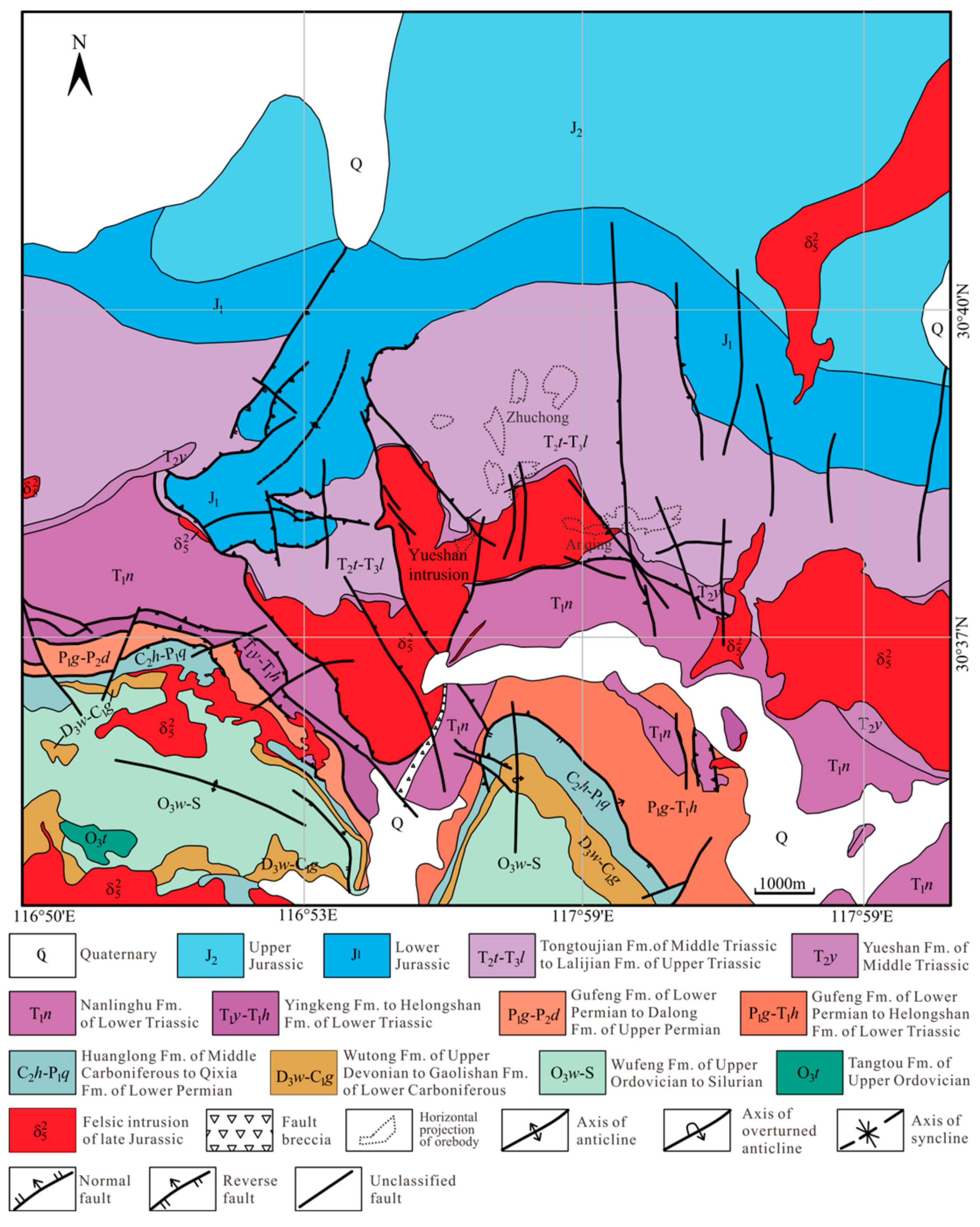
2.1. Geological Setting
2.2. Ore Deposits
3. Methods and Algorithms
3.1. TIN and DSI Methods for Modeling Geological Factors
3.2. Interpolation Algorithms for 3D Block Modeling
3.3. The WofE Method for 3D Spatial Analysis
4. Spatial Association of Intrusion, Resistivity and Volume Strain Fields with Orebodies
4.1. 3D Spatial Association of the Yueshan Intrusion with Orebodies
- (1)
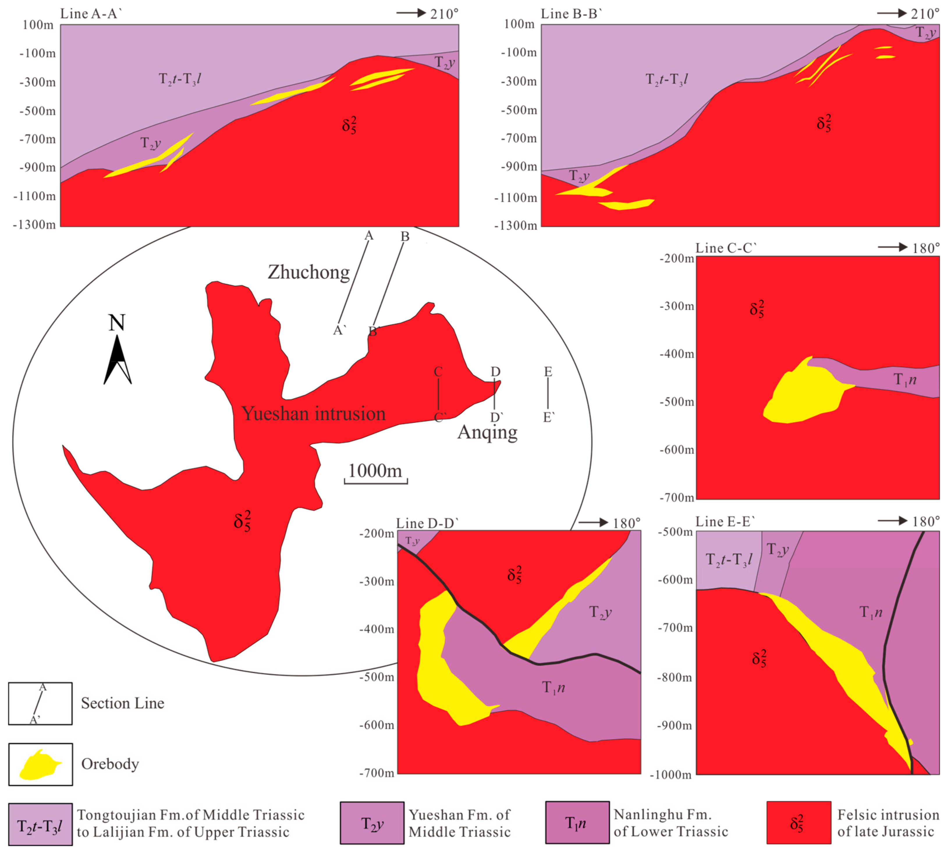
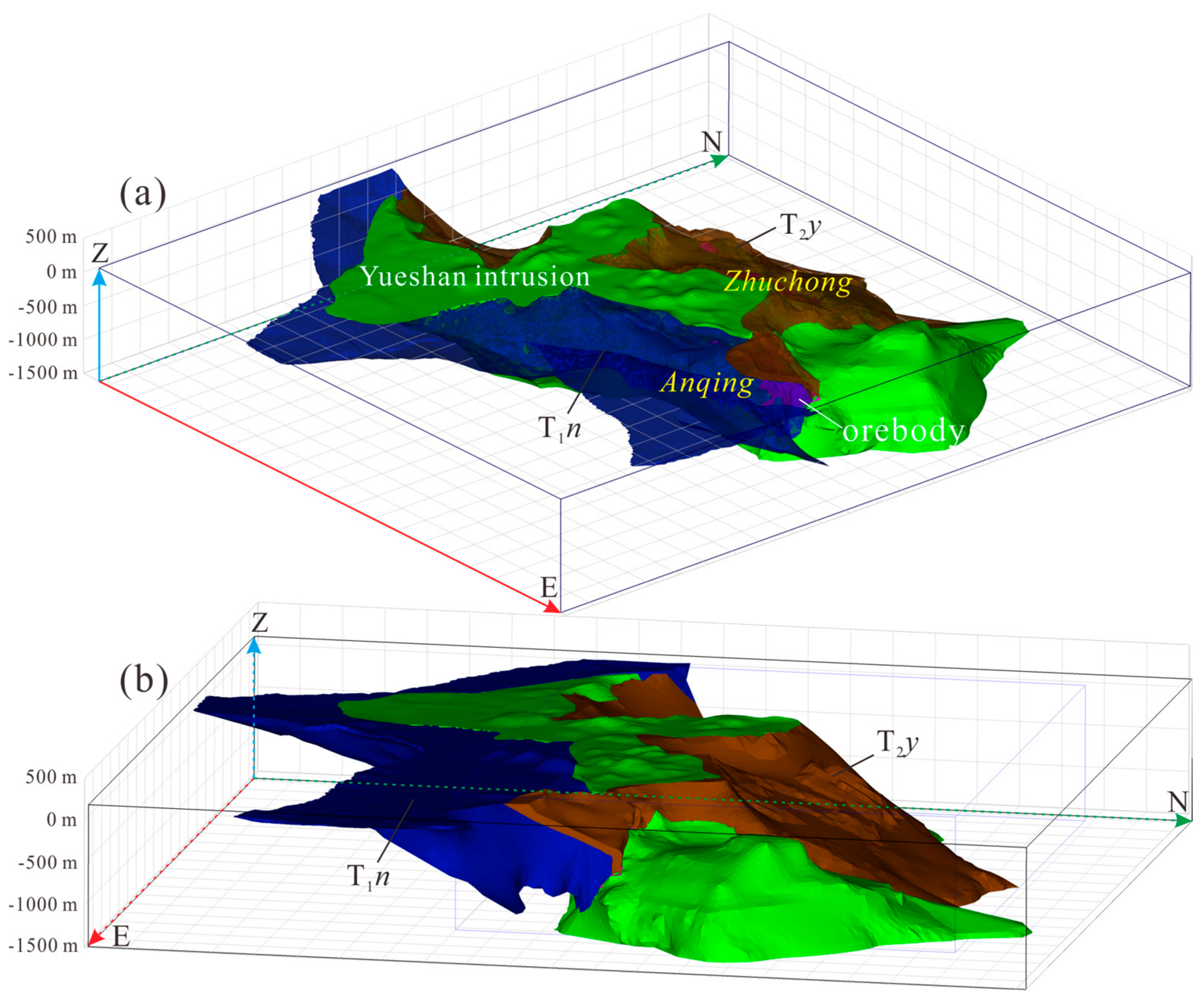
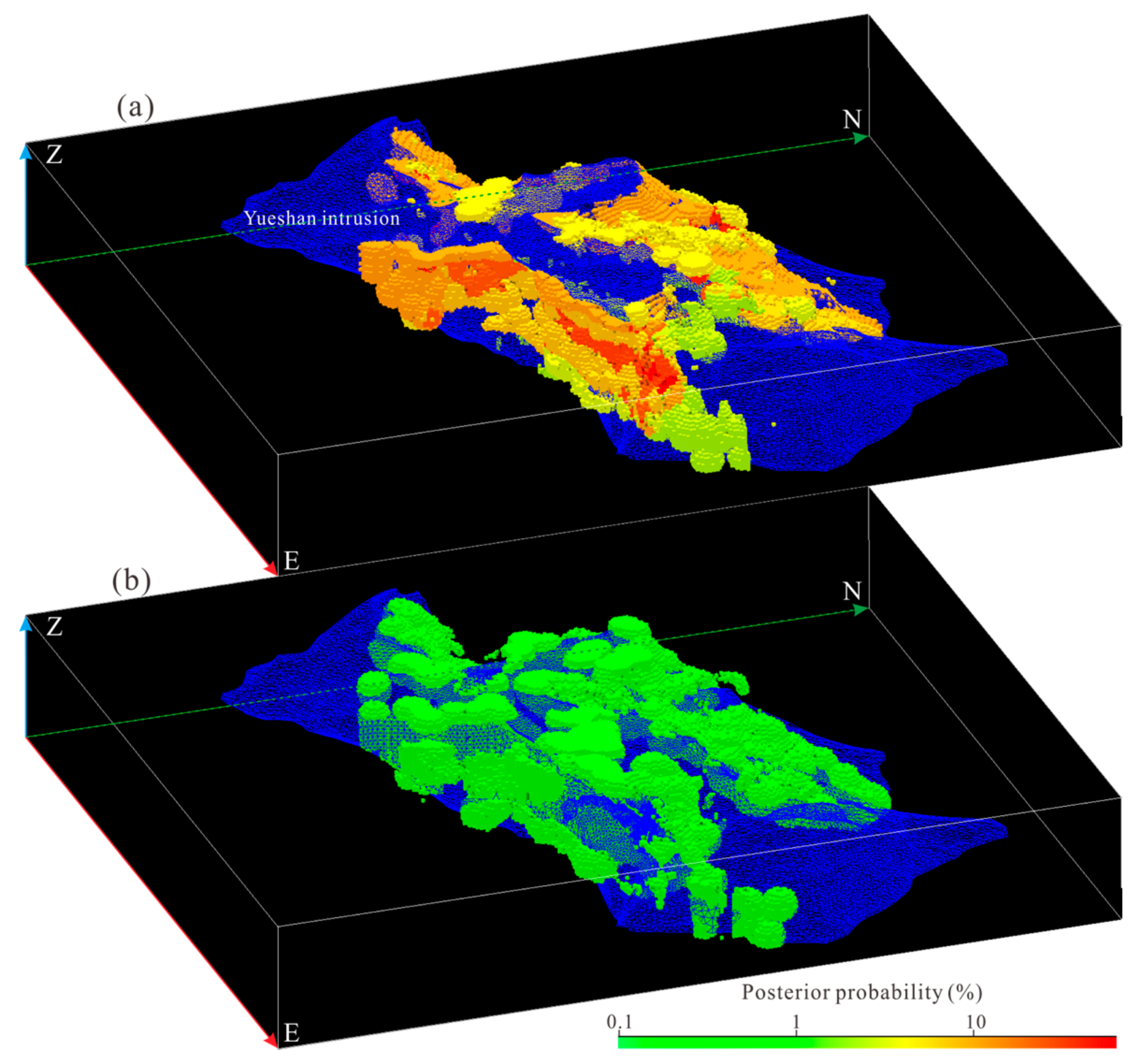
- The 3D Yueshan intrusion exhibits extreme variation in attitude and topography of its contact zone, and such variations have strong constraints on uneven localization of orebodies around the intrusion. Both the south contact zone and north contact zone host more than 99% ores in the ore field. Their common feature that is nearly E–W-trending is completely different from both the west and the east contact zone that are nearly S–N-trending (Figure 3a). It suggests that the E–W-trending contact zone is favourable for skarn mineralization.
- (2)
- The south contact zone hosts much more Cu reserves than the north one. It also displays distinct differences from the north one in occurrence and topography. The south contact zone has an extremely irregular surface with a wide range of dips, from northward (inward) 40°–60° to southward (outward) 20°–45°, while the north one has gentle waved surface with a stable northward (outward) tip about 25°–40° (Figure 3b). These suggest that the rapid change of occurrence might have made a difference for Cu mineralization in contact zone of the Yueshan intrusion. Particularly, the south contact zoon is more favourable for formation of orebodies that the north.
- (3)
- Almost all of orebodies are covered by the strata, T1n and T2y. No orebody is distributed in the east branch of the Yueshan intrusion, where no carbonate rock is present. It illustrates that the mineralization is controlled by the presence of carbonate rocks in direct contact with diorite rocks.
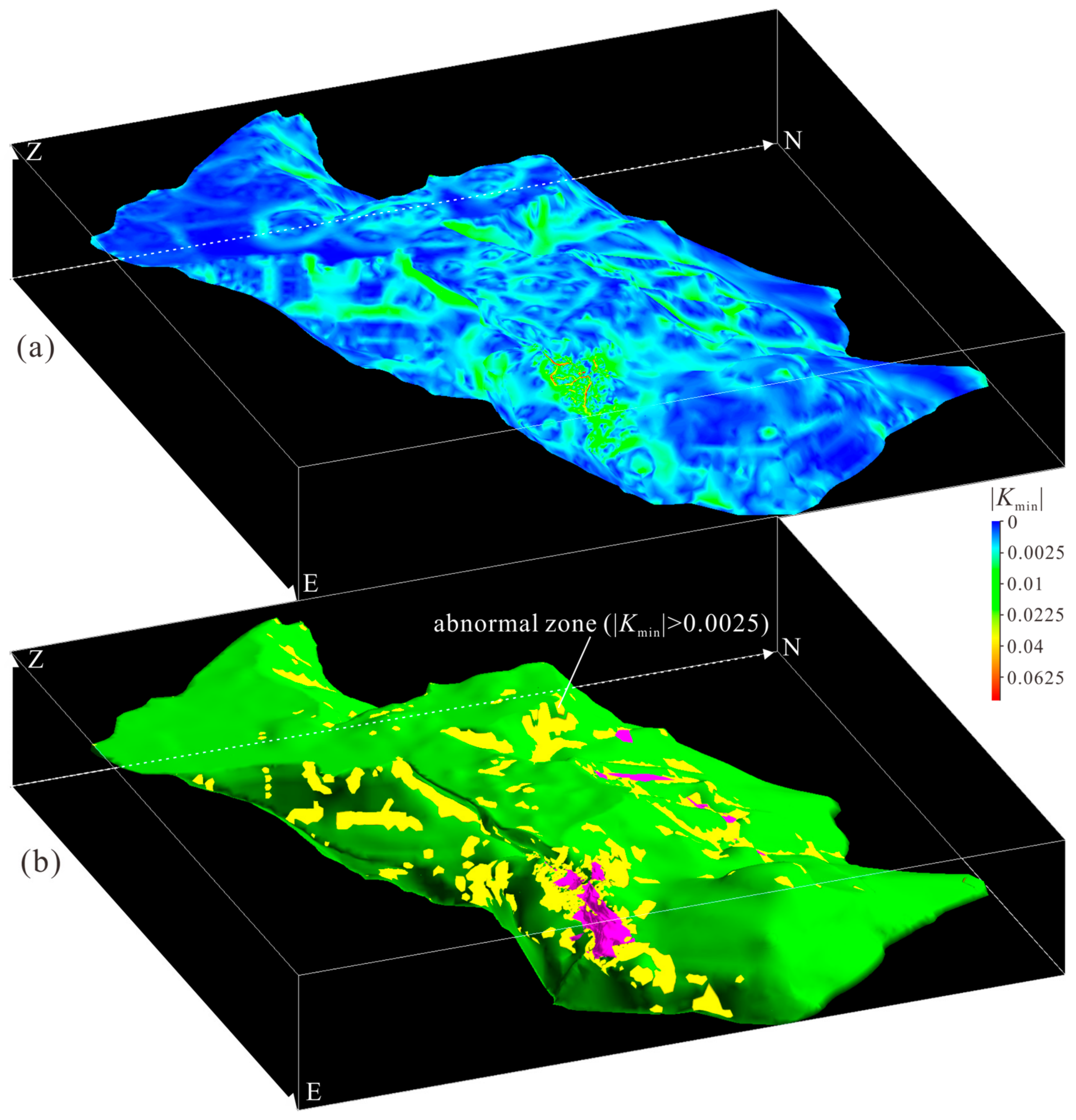
- (4)
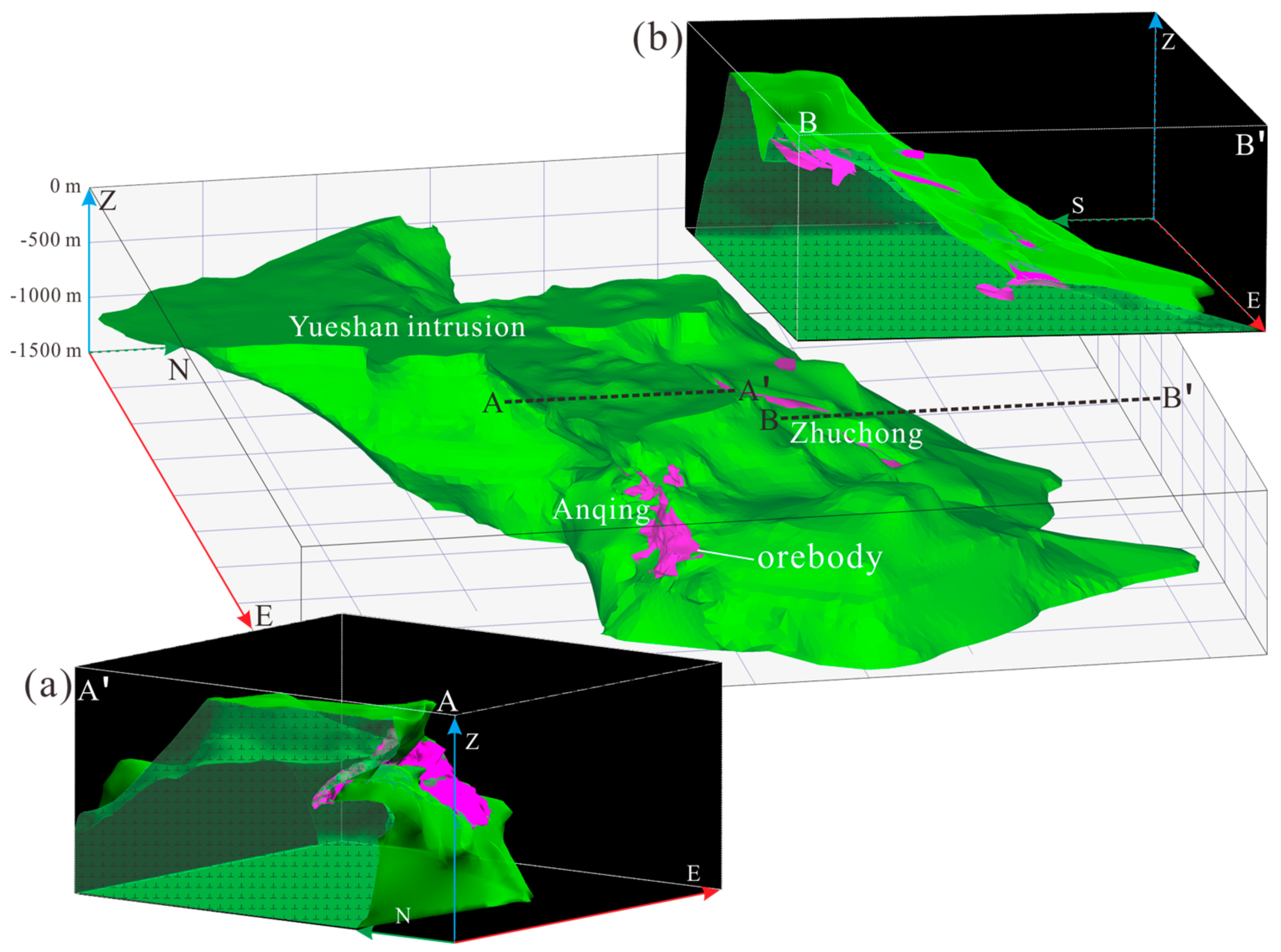
- The orebodies are unevenly localized in the vicinity of the intrusion’s contact zone, especially around the concaves (Figure 4a,b). Remarkably, such uneven localization of orebodies is related to the curvatures [79] of the contact surface. By using the minimum principal curvature (Kmin) to describe the topography of the intrusion’s contact zone (Figure 5a), it is evident that most orebodies are localized around the contact zone with |Kmin| > 0.0025 (Figure 5b).
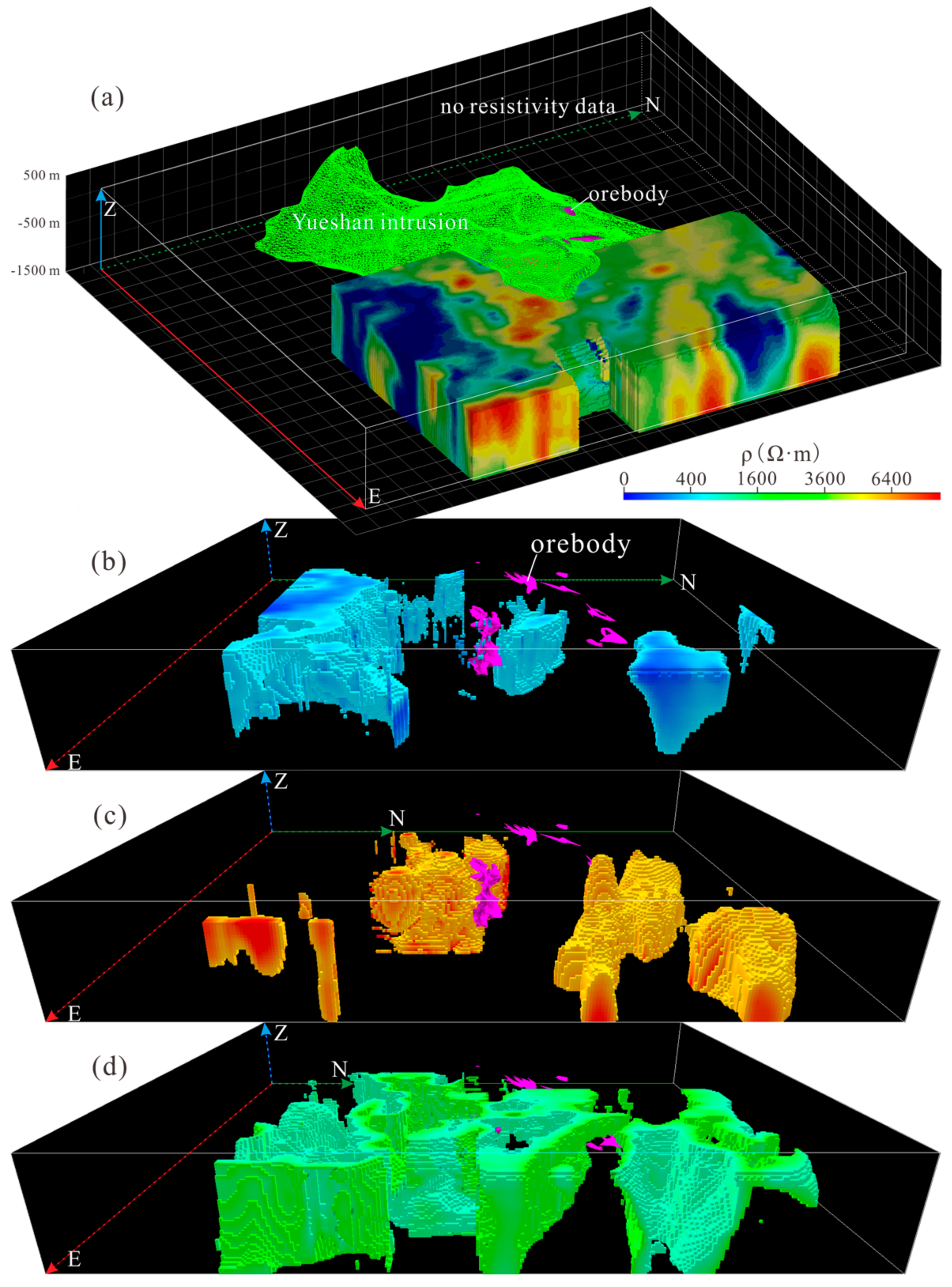
4.2. 3D Resistivity Field and Its Association with Orebodies
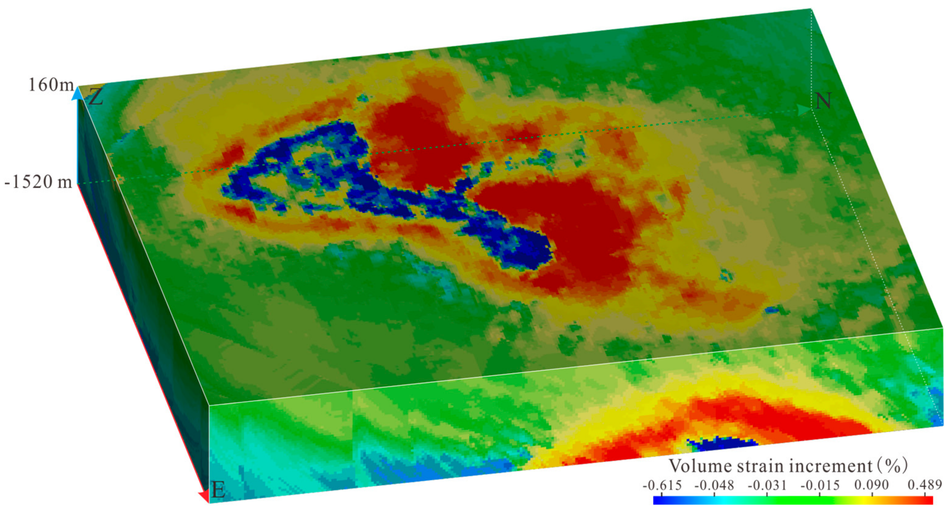
4.3. 3D Volume Strain Field and Its Association with Orebodies
5. Quantitative Integration of Ore-Related Information and Ore Prediction
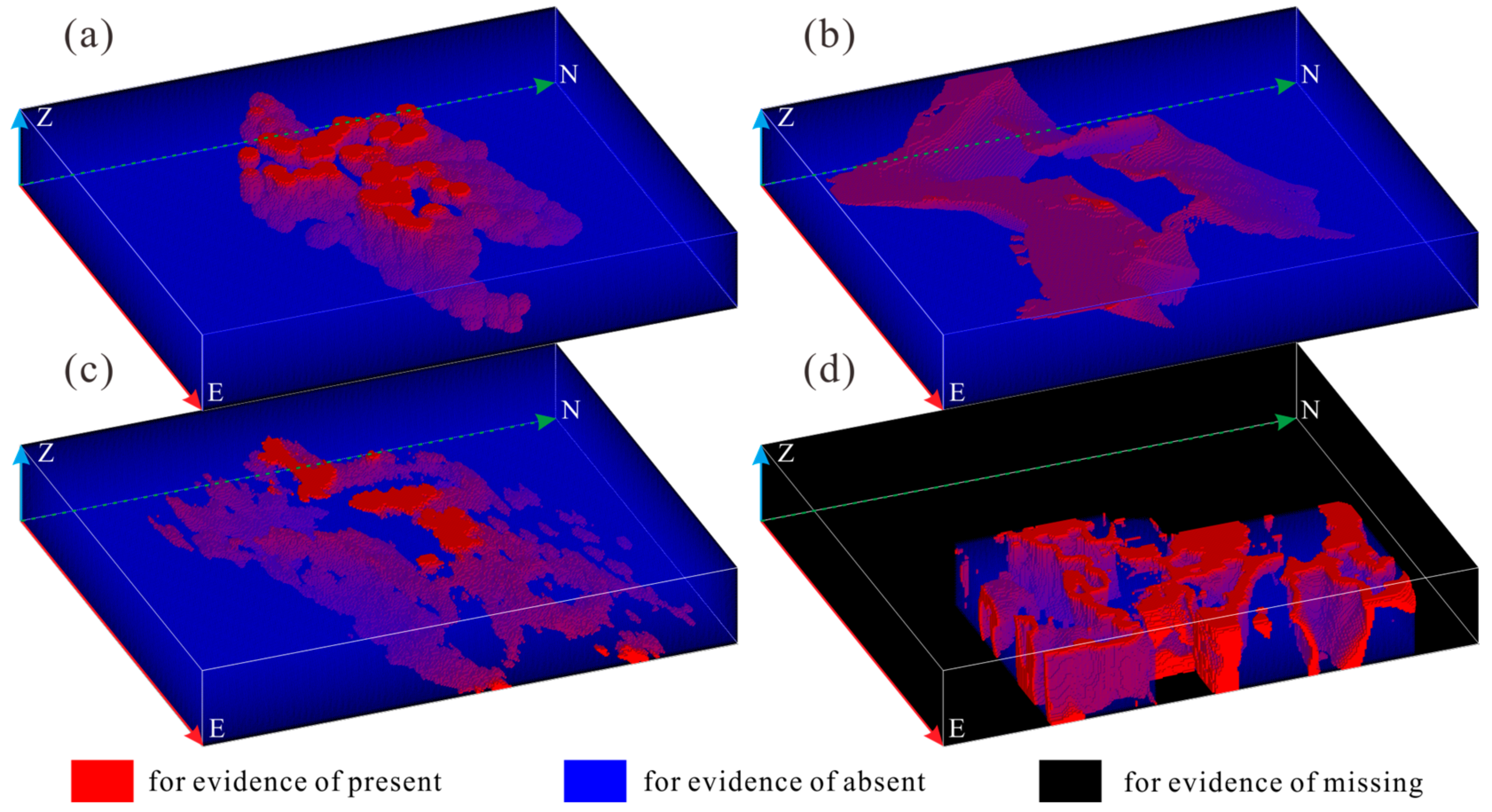
5.1. Binary Predictive Maps of Exploration Criteria
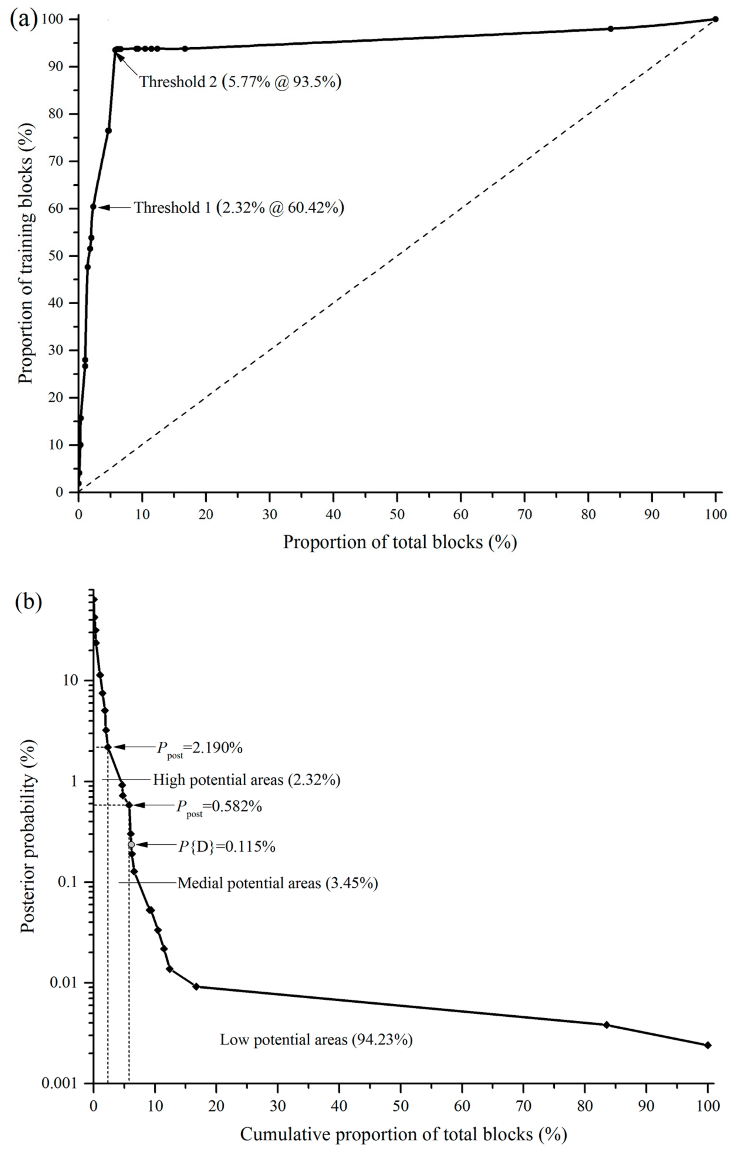
5.2. Prospectivity Mapping and Ore Prediction
6. Conclusions
Author Contributions
Funding
Acknowledgments
Conflicts of Interest
References
- Liu, L.M.; Peng, S.L. Prediction of hidden ore bodies by synthesis of geological, geophysical and geochemical information based on dynamic model in Fenghuangshan ore field, Tongling district, China. J. Geochem. Explor. 2004, 81, 81–98. [Google Scholar] [CrossRef]
- Zhao, P.D. Quantitative mineral prediction and deep mineral exploration. Earth Sci. Front. 2007, 14, 1–10. [Google Scholar]
- Liu, L.M.; Wan, C.L.; Zhao, C.B.; Zhao, Y.L. Geodynamic constraints on orebody localization in the Anqing orefield, China: Computational modeling and facilitating predictive exploration of deep deposits. Ore Geol. Rev. 2011, 43, 249–263. [Google Scholar] [CrossRef]
- Cheng, Q.M. Singularity theory and methods for mapping geochemical anomalies caused by buried sources and for predicting undiscovered mineral deposits in covered areas. J. Geochem. Explor. 2012, 122, 55–70. [Google Scholar] [CrossRef]
- Harris, J.R.; Wilkinson, L.; Grunsky, E.C. Effective use and interpretation of lithogeochemical data in regional mineral exploration programs: Application of Geographic Information Systems (GIS) technology. Ore Geol. Rev. 2000, 16, 107–143. [Google Scholar] [CrossRef]
- Harris, J.R.; Wilkinson, L.; Heather, K.; Fumerton, S.; Bernier, M.A.; Ayer, J.; Dahn, R. Application of GIS Processing Techniques for Producing Mineral Prospectivity Maps-A Case Study: Mesothermal Au in the Swayze Greenstone Belt, Ontario, Canada. Nat. Resour. Res. 2001, 10, 91–124. [Google Scholar] [CrossRef]
- Carranza, E.J.M. Geochemical Anomaly and Mineral Prospectivity Mapping in GIS; Handbook of Exploration & Environmental Geochemistry; Elsevier: New York, NY, USA, 2009; Volume 11, p. 890. [Google Scholar]
- Wu, Q.; Xu, H.; Zou, X.K. An effective method for 3D geological modeling with multi-source data integration. Comput. Geosci. 2005, 31, 35–43. [Google Scholar] [CrossRef]
- Li, N.; Wu, X.C.; Xiao, K.Y.; Chen, X.Q. Rapid voxelization method for complex orebody. J. Huazhong Univ. Sci. Technol. (Nat. Sci. Ed.) 2013, 41, 34–37. [Google Scholar]
- Yang, J. Full 3-D numerical simulation of hydrothermal fluid flow in faulted sedimentary basins: Example of the McArthur Basin, Northern Australia. J. Geochem. Explor. 2006, 89, 440–444. [Google Scholar] [CrossRef]
- Smirnoff, A.; Boisvert, E.; Paradi, S.J. Support vector machine for 3D modeling from sparse geological information of various origins. Comput. Geosci. 2008, 34, 127–143. [Google Scholar] [CrossRef]
- Houlding, S.W. 3D Geoscience Modeling: Computer Techniques for Geological Characterization; Springer: Berlin/Heidelberg, Germany, 1994; 309p. [Google Scholar]
- Christian, J.T. 3D geoscience modeling: Computer techniques for geological characterization. Earth-Sci. Rev. 1996, 40, 299–301. [Google Scholar] [CrossRef]
- Journel, A.G. Geostatistics: Models and tools for the earth sciences. Math. Geol. 1986, 18, 119–140. [Google Scholar] [CrossRef]
- Mallet, J.L. Geomodeling; Oxford University Press: New York, NY, USA, 2002. [Google Scholar]
- Turner, A.K. Challenges and trends for geological modelling and visualisation. Bull. Eng. Geol. Environ. 2006, 65, 109–127. [Google Scholar] [CrossRef]
- Liu, L.M.; Li, J.F.; Zhou, R.C.; Sun, T. 3D modeling of the porphyry-related Dawangding gold deposit in south China: Implications for ore genesis and resources evaluation. J. Geochem. Explor. 2016, 164, 164–185. [Google Scholar] [CrossRef]
- Sanches, A.; Almeida, J.; Sá Caetano, P.; Vieira, R. A 3D Geological Model of a Vein Deposit Built by Aggregating Morphological and Mineral Grade Data. Minerals 2017, 7, 234. [Google Scholar] [CrossRef]
- Agterberg, F. Geomathematics: Theoretical Foundations, Applications and Future Developments; Springer: Berlin, Germany, 2014; 553p. [Google Scholar]
- Silva, D.; Almeida, J. Geostatistical Methodology to Characterize Volcanogenic Massive and Stockwork Ore Deposits. Minerals 2017, 7, 238. [Google Scholar] [CrossRef]
- Schetselaar, E.; Ames, D.; Grunsky, E. Integrated 3D Geological Modeling to Gain Insight in the Effects of Hydrothermal Alteration on Post-Ore Deformation Style and Strain Localization in the FlinFlon Volcanogenic Massive Sulfide Ore System. Minerals 2017, 8, 3. [Google Scholar] [CrossRef]
- Liu, L.M.; Zhao, Y.L.; Sun, T. 3D computational shape- and cooling process-modeling of magmatic intrusion and its implication for genesis and exploration of intrusion-related ore deposits: An example from the Yueshan intrusion in Anqing, China. Tectonophysics 2012, 526, 110–123. [Google Scholar] [CrossRef]
- Kreveld, M.V.; Löffler, M.; Silveira, R.I. Optimization for first order Delaunay triangulations. Comput. Geom. 2010, 43, 377–394. [Google Scholar] [CrossRef]
- Peucker, T.K.; Fowler, R.J.; Little, J.J.; Mark, D.M. The triangulated irregular network. In Proceedings of the Digital Terrain Models Symposium, St. Louis, MO, USA, 9–11 May 1978; pp. 516–540. [Google Scholar]
- Tsai, V.D. Delaunay triangulations in TIN creation: An overview and a linear-time algorithm. Int. J. Geogr. Inf. Syst. 1993, 7, 501–524. [Google Scholar] [CrossRef]
- Mallet, J.L. Discrete smooth interpolation. ACM Trans. Gr. 1989, 8, 121–144. [Google Scholar] [CrossRef]
- Mallet, J.L. Discrete smooth interpolation in geometric modelling. Comput.-Aided Des. 1992, 24, 178–191. [Google Scholar] [CrossRef]
- Lorensen, W.E.; Cline, H.E. Marching cube: A high resolution 3d surface construction algorithm. Comput. Gr. 1987, 21, 163–169. [Google Scholar] [CrossRef]
- Shepard, D. A two-dimensional interpolation function for irregularly-spaced data. In Proceedings of the 1968 23rd ACM National Conference, Las Vegas, NV, USA, 27–29 August 1968; pp. 517–524. [Google Scholar]
- Bartier, P.M.; Keller, C.P. Multivariate interpolation to incorporate thematic surface data using inverse distance weighting (idw). Comput. Geosci. 1996, 22, 795–799. [Google Scholar] [CrossRef]
- Stein, M.L. Interpolation of Spatial Data: Some Theory for Kriging; Springer: New York, NY, USA, 1999; 249p. [Google Scholar]
- Yamamoto, J.K. Correcting the smoothing effect of ordinary kriging estimates. Math. Geol. 2005, 37, 69–94. [Google Scholar] [CrossRef]
- Adeli, A.; Emery, X.; Dowd, P. Geological Modelling and Validation of Geological Interpretations via Simulation and Classification of Quantitative Covariates. Minerals 2018, 8, 7. [Google Scholar] [CrossRef]
- Carranza, E.J.M. Controls on mineral deposit occurrence inferred from analysis of their spatial pattern and spatial association with geological features. Ore Geol. Rev. 2009, 35, 383–400. [Google Scholar] [CrossRef]
- Yuan, F.; Li, X.H.; Zhang, M.M.; Jowitt, S.M.; Jia, C.; Zheng, T.K.; Zhou, T.F. Three-dimensional weights of evidence-based prospectivity modeling: A case study of the Baixiangshan mining area, Ningwu Basin, Middle and Lower Yangtze Metallogenic Belt, China. J. Geochem. Explor. 2014, 145, 82–97. [Google Scholar] [CrossRef]
- Li, N.; Bagas, L.; Li, X.H.; Xiao, K.Y.; Li, Y.; Ying, L.J.; Song, X.L. An improved buffer analysis technique for model-based 3d mineral potential mapping and its application. Ore Geol. Rev. 2016, 76, 94–107. [Google Scholar] [CrossRef]
- Malehmir, A.; Thunehed, H.; Tryggvason, A. The Paleoproterozoic Kristineberg mining area, northern Sweden: Results from integrated 3D geophysical and geologic modelling, and implications for targeting ore deposits. Geophysics 2009, 74, B9–B22. [Google Scholar] [CrossRef]
- Perrouty, S.; Lindsay, M.D.; Jessell, M.W.; Aillères, L.; Martin, R.; Bourassa, Y. 3D modeling of the Ashanti Belt, southwest Ghana: Evidence for a litho-stratigraphic control on gold occurrences within the Birimian Sefwi Group. Ore Geol. Rev. 2014, 63, 252–264. [Google Scholar] [CrossRef]
- Nielsen, S.H.; Cunningham, F.; Hay, R.; Partington, G.; Stokes, M. 3D prospectivity modelling of orogenic gold in the Marymia Inlier, Western Australia. Ore Geol. Rev. 2015, 7, 578–591. [Google Scholar] [CrossRef]
- Xiao, K.Y.; Li, N.; Porwal, A.; Holden, E.J.; Bagas, L.; Lu, Y.J. Research on gis-based 3d prospectivity mapping and a case study of jiama copper-polymetallic deposit in tibet, china. Ore Geol. Rev. 2015, 71, 611–632. [Google Scholar] [CrossRef]
- Dubois, D.; Hájek, P.; Prade, H. Knowledge-Driven versus Data-Driven Logics. J. Log. Lang. Inf. 2000, 9, 65–89. [Google Scholar] [CrossRef]
- Liu, L.M.; Peng, S.L. Key strategies for predictive exploration in mature environment: Model innovation, exploration technology optimization and information integration. J. Cent. South Univ. Technol. 2005, 12, 186–191. [Google Scholar] [CrossRef]
- D’Ercole, C.; Groves, D.I.; Knox-Robinson, C.M. Using fuzzy logic in a Geographic Information System environment to enhance conceptually based prospectivity analysis of Mississippi Valley-type mineralisation. Aust. J. Earth Sci. 2000, 47, 913–927. [Google Scholar] [CrossRef]
- Rencz, A.N. Data integration for mineral exploration in the Antigonish Highlands, Nova Scotia: Application of GIS and remote sensing. Can. J. Remote Sens. 1994, 20, 257–267. [Google Scholar]
- Roddy, R.K.T.; Bonham-Carter, G.F. A decision-tree approach to mineral potential mapping in Snow Lake area, Mantitoba. Can. J. Remote Sens. 1991, 17, 191–200. [Google Scholar] [CrossRef]
- Bonham-Carter, G.F.; Agterberg, F.P.; Wright, D.F. Weights of evidence modeling: A new approach to mapping mineral potential. Geol. Surv. Canada 1989, 89, 171–183. [Google Scholar]
- Agterberg, F.P.; Bonham-Carter, G.F.; Wright, D.F. Statistical Pattern Integration for Mineral Exploration. Comput. Appl. Resour. Estim. 1990, 1–21. [Google Scholar] [CrossRef]
- Chung, C.F.; Agterberg, E.P. Regression models for estimating mineral resources from geological map data. Math. Geol. 1980, 12, 473–488. [Google Scholar] [CrossRef]
- Brown, W.M.; Gedeon, T.D.; Groves, D.I.; Barnes, R.G. Artificial neural networks: A new method for mineral prospectivity mapping. Aust. J. Earth Sci. 2015, 7, 757–770. [Google Scholar] [CrossRef]
- Bonham-Carter, G.F.; Agterberg, F.P.; Wright, D.F. Integration of Geological Datasets for Gold Exploration in Nova Scotia. Photogramm. Eng. Remote Sens. 1990, 54, 1585–1592. [Google Scholar]
- Cheng, Q.M.; Agterberg, F.P. Fuzzy weights of evidence method and its plication in mineral potential mapping. Nat. Resour. Res. 1999, 8, 27–35. [Google Scholar] [CrossRef]
- Carranza, E.J.M. Weights of Evidence Modeling of Mineral Potential: A Case Study Using Small Number of Prospects, Abra, Philippines. Nat. Resour. Res. 2004, 13, 173–187. [Google Scholar] [CrossRef]
- Lu, Y.; Liu, L.M.; Xu, G.J. Constraints of deep crustal structures on large deposits in the Cloncurry district, Australia: Evidence from spatial analysis. Ore Geol. Rev. 2016, 79, 316–331. [Google Scholar] [CrossRef]
- Sun, T.; Wu, K.; Chen, L.; Liu, W.; Wang, Y.; Zhang, C. Joint Application of Fractal Analysis and Weights-of-Evidence Method for Revealing the Geological Controls on Regional-Scale Tungsten Mineralization in Southern Jiangxi Province, China. Minerals 2017, 7, 243. [Google Scholar] [CrossRef]
- Zhao, Y.M. Skarn deposits in the circum-pacific belt. Miner. Depos. 1991, 10, 41–51, (In Chinese with English Abstract). [Google Scholar]
- Lentz, D.R. Carbonatite genesis: A reexamination of the role of intrusion-related pneumatolytic skarn processes in limestone melting. Geology 1999, 27, 335. [Google Scholar] [CrossRef]
- Pan, Y.; Dong, P. The lower chanjiang (yangzi/yangzte river) metallogenic belt, east china: Intrusion- and wall rock-hosted cu-fe-au, mo, zn, pb and ag deposits. Ore Geol. Rev. 1999, 15, 177–242. [Google Scholar] [CrossRef]
- Chang, Y.F.; Liu, X.P.; Wu, Y.C. The Copper–Iron Belt of the Low and Middle Reaches of the Yangtze River; Geological Publish House: Beijing, China, 1991; p. 359. (In Chinese) [Google Scholar]
- Dong, S.W.; Qiu, R.L. Tectonism and Magmatism in the Anqing-Yueshan Area; Geological Publishing House: Beijing, China, 1993; p. 154. (In Chinese) [Google Scholar]
- Wang, X.C.; Zhou, Y.C. Geological characteristics and origin of Anqing Cu–Fe deposit, Anhui. Geol. Prospect. 1995, 31, 16–23, (In Chinese with English Abstract). [Google Scholar]
- Liu, L.M.; Shu, Z.M.; Zhao, C.B.; Wan, C.L.; Cai, A.L.; Zhao, Y.L. The controlling mechanism of ore formation due to flow-focusing dilation spaces in skarn ore deposits and its significances for deep-ore exploration: Examples from the Tongling-Anqing district. Acta Petrol. Sin. 2008, 24, 1848–1856, (In Chinese with English Abstract). [Google Scholar]
- Mao, J.W.; Wang, Y.T.; Lehmann, B.; Yu, J.J.; Du, A.D.; Mei, Y.X.; Li, Y.F.; Zang, W.S.; Stein, H.J.; Zhou, T.F. Molybdenite Re–Os and albite 40Ar/39Ar dating of Cu–Au–Mo and magnetite porphyry systems in the Yangtze River valley and metallogenic implications. Ore Geol. Rev. 2006, 29, 307–324. [Google Scholar] [CrossRef]
- Zhou, T.F.; Yuan, F.; Yue, SC.; Liu, X.D.; Zhang, X.; Fan, Y. Geochemistry and evolution of ore-forming fluids of the Yueshan Cu–Au skarn-and vein-type deposits, Anhui Province, South China. Ore Geol. Rev. 2007, 31, 279–303. [Google Scholar] [CrossRef]
- Zhang, L.J.; Zhou, T.F.; Fan, Y.; Yuan, F. SHRIMP U–Pb zircon dating of Yueshan intrusion in the Yueshan ore field, Anhui, and its significance. Acta Petrol. Sin. 2008, 24, 1725–1732, (In Chinese with English Abstract). [Google Scholar]
- Liu, Z.F.; Shao, Y.J.; Shu, Z.M. Rock-forming mechanism of Yueshan intrusion, Tongling, Anhui Province. China. Chin. J. Nonferr. Met. 2012, 22, 652–659, (In Chinese with English Abstract). [Google Scholar]
- Liu, Z.F.; Shao, Y.J.; Shu, Z.M.; Peng, N.H.; Xie, Y.L.; Zhang, Y. Fluid inclusion characteristics of Longmenshan copper-polymetallic deposit in Yueshan, Anhui Province, China. J. Cent. South Univ. 2012, 19, 2627–2633. [Google Scholar] [CrossRef]
- Liu, Z.F.; Shao, Y.J.; Zhang, J.D.; Shu, Z.M.; Zhang, Y. Magma source and evolution law in Yueshan ore field, Anhui Province, China. J. Cent. South Univ. 2014, 21, 1491–1498. [Google Scholar] [CrossRef]
- Zhao, Y.L.; Liu, L.M.; Cai, A.L.; Zou, C. Three-Dimensional Geometry of the Contact Zone in the Anqing Copper Deposit, Anhui Province and Its Ore-Controlling Mechanism. Geol. Explor. 2010, 46, 649–656. [Google Scholar]
- Liu, L.M.; Zhou, R.C.; Zhao, C.B. Constraints of tectonic stress regime on mineralization system related to the hypabyssal intrusion: Implication from the computational modeling experiments on the geodynamics during cooling process of the Yuenshan intrusion in Anqing district, China. Acta Petrol. Sin. 2010, 26, 2869–2878, (In Chinese with English Abstract). [Google Scholar]
- Wu, Q.; Xu, H. An approach to computer modeling and visualization of geological faults in 3D. Comput. Geosci. 2003, 29, 503–509. [Google Scholar] [CrossRef]
- Caumon, G.; Collon-Drouaillet, P.; de Veslud, C.L.C.; Viseur, S.; Sausse, J. Surface-Based 3D Modeling of Geological Structures. Math. Geosci. 2009, 41, 927–945. [Google Scholar] [CrossRef]
- Hassen, I.; Gibson, H.; Hamzaoui-Azaza, F.; Negrod, F.; Rachide, K. 3D geological modeling of the Kasserine Aquifer System, Central Tunisia: New insights into aquifer-geometry and interconnections for a better assessment of groundwater resources. J. Hydrol. 2016, 539, 223–236. [Google Scholar] [CrossRef]
- Jay, L. Comparison of existing methods for building triangular irregular network, models of terrain from grid digital elevation models. Geogr. Inf. Syst. 1991, 5, 267–285. [Google Scholar]
- Bern, M.; Eppstein, D.; Gilbert, J. Provably good mesh generation. J. Comput. Syst. Sci. 1994, 48, 384–409. [Google Scholar] [CrossRef]
- Pollen, D.A.; Ronner, S.F. Phase relationships between adjacent simple cells in the visual cortex. Science 1981, 212, 1409–1411. [Google Scholar] [CrossRef] [PubMed]
- Cohen-Or, D.; Kaufman, A. Fundamentals of Surface Voxelization. Gr. Models Image Process. 1995, 57, 453–461. [Google Scholar] [CrossRef]
- Couprie, M.; Coeurjolly, D.; Zrour, R. Discrete bisector function and Euclidean skeleton in 2D and 3D. Image Vis. Comput. 2007, 25, 1543–1556. [Google Scholar] [CrossRef]
- Porwal, A.; Gonzalez-Alvarez, I.; Markwitz, V.; McCuaig, T.C.; Mamuse, A. Weights-of evidence and logistic regression modelling ofmagmatic nickel sulfide prospectivity in the Yilgarn Craton, Western Australia. Ore Geol. Rev. 2010, 38, 184–196. [Google Scholar] [CrossRef]
- Koenderink, J.J.; Doorn, A.J.V. Surface shape and curvature scales. Image Vis. Comput. 1993, 10, 557–564. [Google Scholar] [CrossRef]
- Wu, H. Problem of buffer zone construction in gis. J. Wuhan Tech. Univ. Surv. Mapp. 1997, 22, 358–366, (In Chinese with English Abstract). [Google Scholar]
- Bonham-Carter, G.F. Geographic Information System for Geoscientists, Modeling with GIS; Pergamon: New York, NY, USA, 1994; pp. 238–333. [Google Scholar]
- Porwal, A.; Carranza, E.J.M. Classifiers for modelling of mineral potential. In Bayesian Networks: A Practical Guide to Applications; Pourret, O., Naïm, P., Marcot, B., Eds.; John Wiley & Sons: Chichester, UK, 2008; pp. 149–171. [Google Scholar]


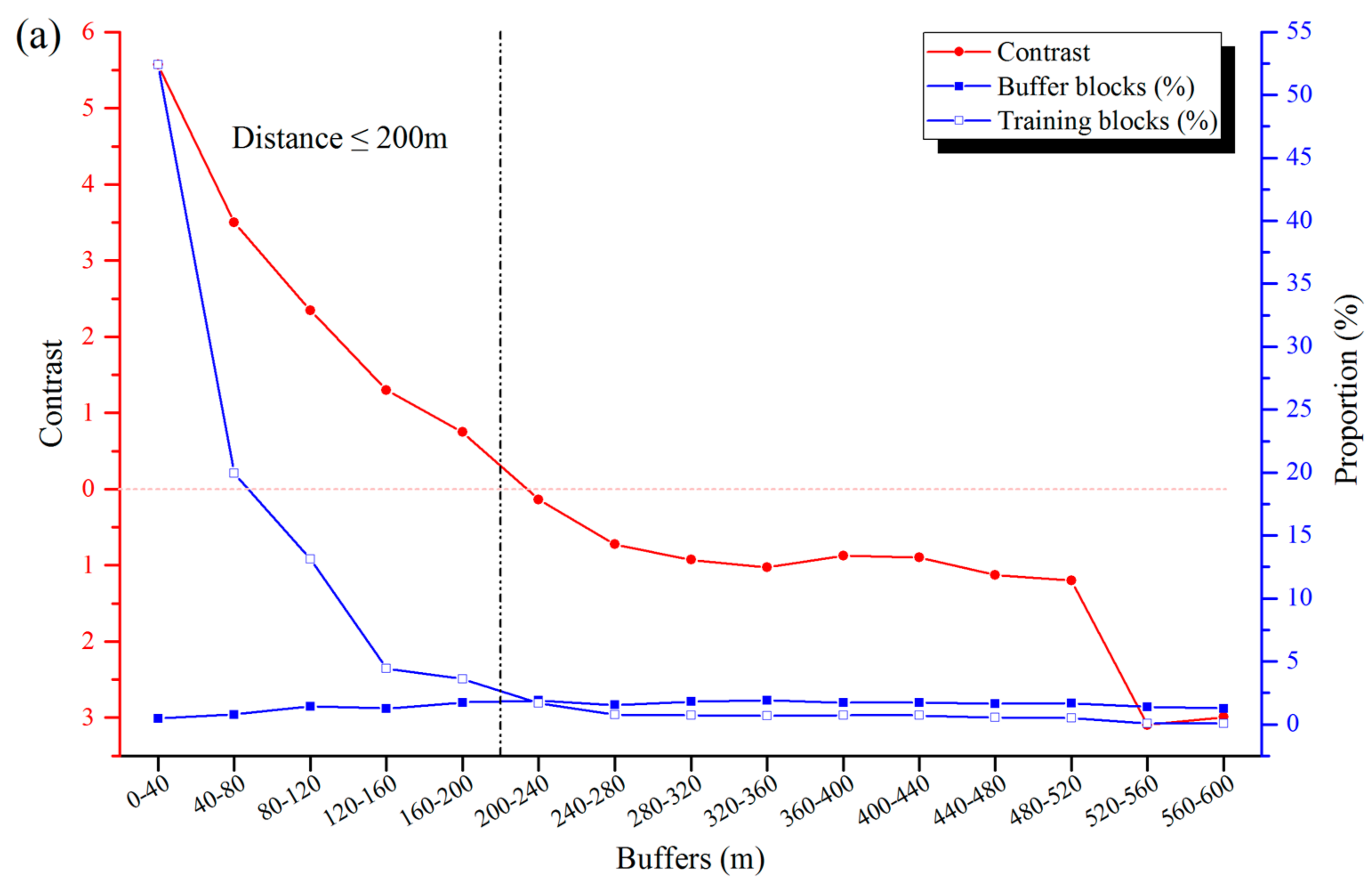
| Buffer Distance (m) | Training Blocks | 3D Buffers Blocks | Positive Weight | Negative Weight | Contrast |
|---|---|---|---|---|---|
| 0–40 | 1670 | 13,257 | 4.833 | −0.739 | 5.572 |
| 40–80 | 635 | 21,356 | 3.285 | −0.215 | 3.5 |
| 80–120 | 419 | 39,987 | 2.223 | −0.127 | 2.349 |
| 120–160 | 142 | 35,011 | 1.267 | −0.033 | 1.3 |
| 160–200 | 115 | 48,498 | 0.729 | −0.019 | 0.748 |
| 200–240 | 53 | 52,795 | −0.132 | 0.002 | −0.135 |
| 240–280 | 24 | 42,926 | −0.718 | 0.008 | −0.726 |
| 280–320 | 23 | 50,185 | −0.917 | 0.011 | −0.928 |
| 320–360 | 22 | 53,040 | −1.017 | 0.012 | −1.029 |
| 360–400 | 23 | 47,611 | −0.864 | 0.01 | −0.874 |
| 400–440 | 23 | 48,613 | −0.885 | 0.01 | −0.896 |
| 440–480 | 17 | 45,318 | −1.117 | 0.011 | −1.128 |
| 480–520 | 16 | 46,371 | −1.201 | 0.012 | −1.213 |
| 520–560 | 2 | 38,500 | −3.095 | 0.013 | −3.108 |
| 560–600 | 2 | 34,698 | −2.991 | 0.012 | −3.003 |
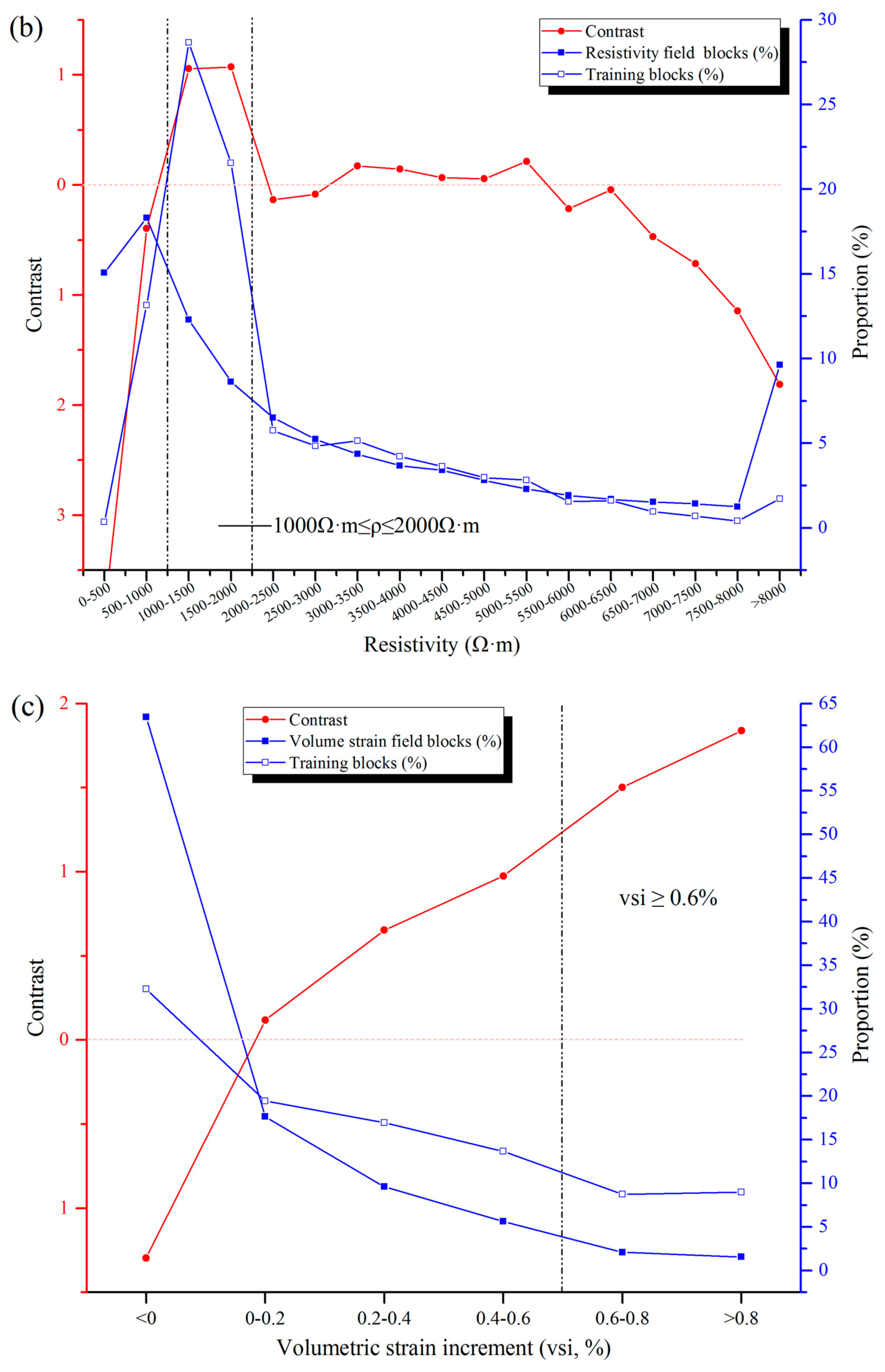
| Resistivity (Ω·m) | Training Blocks | Resistivity Field Blocks | Positive Weight | Negative Weight | Contrast |
|---|---|---|---|---|---|
| 0–500 | 7 | 108,326 | −3.757 | 0.160 | −3.917 |
| 500–1000 | 261 | 131,683 | −0.332 | 0.061 | −0.393 |
| 1000–1500 | 569 | 88,472 | 0.850 | −0.207 | 1.056 |
| 1500–2000 | 428 | 62,106 | 0.919 | −0.153 | 1.072 |
| 2000–2500 | 114 | 46,792 | −0.125 | 0.008 | −0.133 |
| 2500–3000 | 96 | 37,656 | −0.080 | 0.004 | −0.084 |
| 3000–3500 | 102 | 31,350 | 0.165 | −0.008 | 0.173 |
| 3500–4000 | 84 | 26,459 | 0.140 | −0.006 | 0.146 |
| 4000–4500 | 72 | 24,442 | 0.065 | −0.002 | 0.068 |
| 4500–5000 | 59 | 20,238 | 0.055 | −0.002 | 0.056 |
| 5000–5500 | 56 | 16,482 | 0.208 | −0.005 | 0.214 |
| 5500–6000 | 31 | 13,868 | −0.212 | 0.004 | −0.215 |
| 6000–6500 | 32 | 12,117 | −0.044 | 0.001 | −0.045 |
| 6500–7000 | 19 | 10,945 | −0.465 | 0.006 | −0.471 |
| 7000–7500 | 14 | 10,260 | −0.706 | 0.007 | −0.713 |
| 7500–8000 | 8 | 9005 | −1.136 | 0.009 | −1.144 |
| greater than 8000 | 34 | 69,258 | −1.729 | 0.084 | −1.813 |
| Vsi (%) | Training Blocks | Volume Strain Field Blocks | Positive Weight | Negative Weight | Contrast |
|---|---|---|---|---|---|
| less than 0 | 1027 | 1,764,862 | −0.678 | 0.618 | −1.296 |
| 0–0.2 | 619 | 490,349 | 0.097 | −0.022 | 0.119 |
| 0.2–0.4 | 540 | 267,098 | 0.569 | −0.085 | 0.654 |
| 0.4–0.6 | 435 | 156,733 | 0.886 | −0.089 | 0.975 |
| 0.6–0.8 | 279 | 58,388 | 1.432 | −0.071 | 1.502 |
| greater than 0.8 | 286 | 43,096 | 1.762 | −0.078 | 1.838 |
| Evidential Factors | Exploration Criterion | Favourable Range for BPM 1 | Conditional Probability (%) | Positive Weight | Negative Weight | Contrast |
|---|---|---|---|---|---|---|
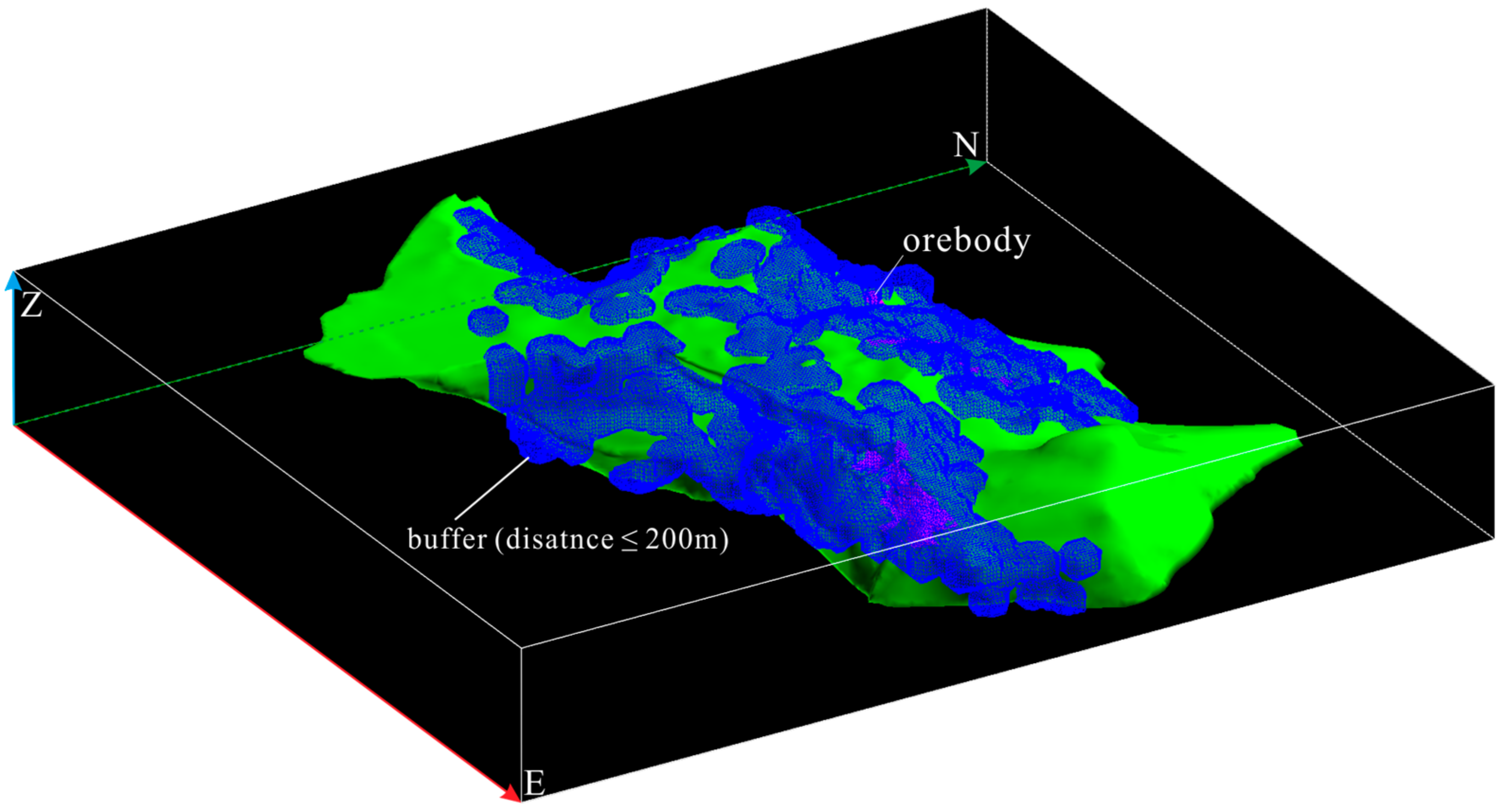
| Contact zone of the Yueshan intrusion | B: 3D buffers (around chosen contact zones) | 0–200 (m) | 1.884 | 2.818 | −2.676 | 5.494 |
| Stratigraphy | C: carbonate | T1n and T2y | 0.896 | 2.064 | −0.567 | 2.631 |
| 3D volume strain field | V: volumetric strain increment | greater than 0.6% | 0.655 | 1.584 | −0.158 | 1.742 |
| 3D resistivity field | R: resistivity | 1000–2000 (Ω·m) | 0.556 | 0.869 | −0.453 | 1.322 |
| CofBPMs 1 | Posterior Probability (%) | Training Blocks | Total Blocks |
|---|---|---|---|
| B+C+V+R+ | 64.003 | 60 | 355 |
| B+C+V+R0 | 42.476 | 71 | 3604 |
| B+C+V+R− | 31.720 | 190 | 4925 |
| B+C+V−R+ | 23.722 | 180 | 2215 |
| B+C+V−R0 | 11.438 | 350 | 18,077 |
| B+C−V+R+ | 11.346 | 41 | 296 |
| B+C+V−R− | 7.515 | 626 | 11,334 |
| B+C−V+R0 | 5.047 | 125 | 10,568 |
| B+C−V+R− | 3.236 | 72 | 5034 |
| B+C−V−R+ | 2.190 | 210 | 8168 |
| B+C−V−R0 | 0.921 | 511 | 65,414 |
| B−C+V+R+ | 0.726 | 0 | 2456 |
| B+C−V−R− | 0.581 | 543 | 28,119 |
| B−C+V+R0 | 0.303 | 6 | 7490 |
| B−C+V+R− | 0.191 | 0 | 5551 |
| B−C+V−R+ | 0.128 | 0 | 9270 |
| B−C+V−R0 | 0.053 | 3 | 70,145 |
| B−C−V+R+ | 0.053 | 0 | 7794 |
| B−C+V−R− | 0.033 | 0 | 30,461 |
| B−C−V+R0 | 0.022 | 0 | 27,843 |
| B−C−V+R− | 0.014 | 0 | 25,708 |
| B−C−V−R+ | 0.009 | 0 | 120,053 |
| B−C−V−R0 | 0.004 | 134 | 1,857,926 |
| B−C−V−R− | 0.002 | 64 | 457,720 |
© 2018 by the authors. Licensee MDPI, Basel, Switzerland. This article is an open access article distributed under the terms and conditions of the Creative Commons Attribution (CC BY) license (http://creativecommons.org/licenses/by/4.0/).
Share and Cite
Qin, Y.; Liu, L. Quantitative 3D Association of Geological Factors and Geophysical Fields with Mineralization and Its Significance for Ore Prediction: An Example from Anqing Orefield, China. Minerals 2018, 8, 300. https://doi.org/10.3390/min8070300
Qin Y, Liu L. Quantitative 3D Association of Geological Factors and Geophysical Fields with Mineralization and Its Significance for Ore Prediction: An Example from Anqing Orefield, China. Minerals. 2018; 8(7):300. https://doi.org/10.3390/min8070300
Chicago/Turabian StyleQin, Yaozu, and Liangming Liu. 2018. "Quantitative 3D Association of Geological Factors and Geophysical Fields with Mineralization and Its Significance for Ore Prediction: An Example from Anqing Orefield, China" Minerals 8, no. 7: 300. https://doi.org/10.3390/min8070300
APA StyleQin, Y., & Liu, L. (2018). Quantitative 3D Association of Geological Factors and Geophysical Fields with Mineralization and Its Significance for Ore Prediction: An Example from Anqing Orefield, China. Minerals, 8(7), 300. https://doi.org/10.3390/min8070300