
Particle Flow Characteristics and Transportation Optimization of Superfine Unclassified Backfilling

Abstract
:1. Introduction
2. Research Objectives and Methods
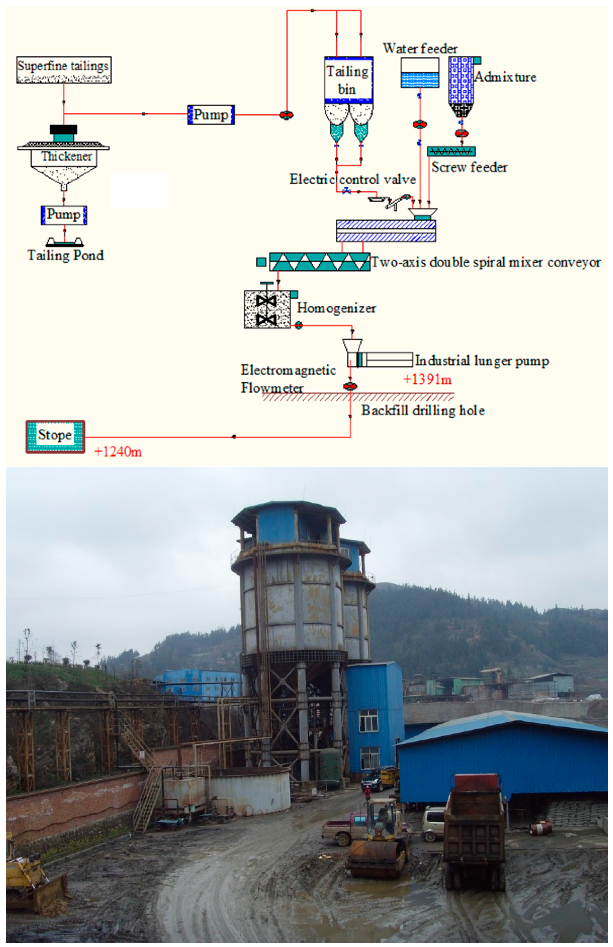
2.1. Project Description
2.2. Model Computational Domain
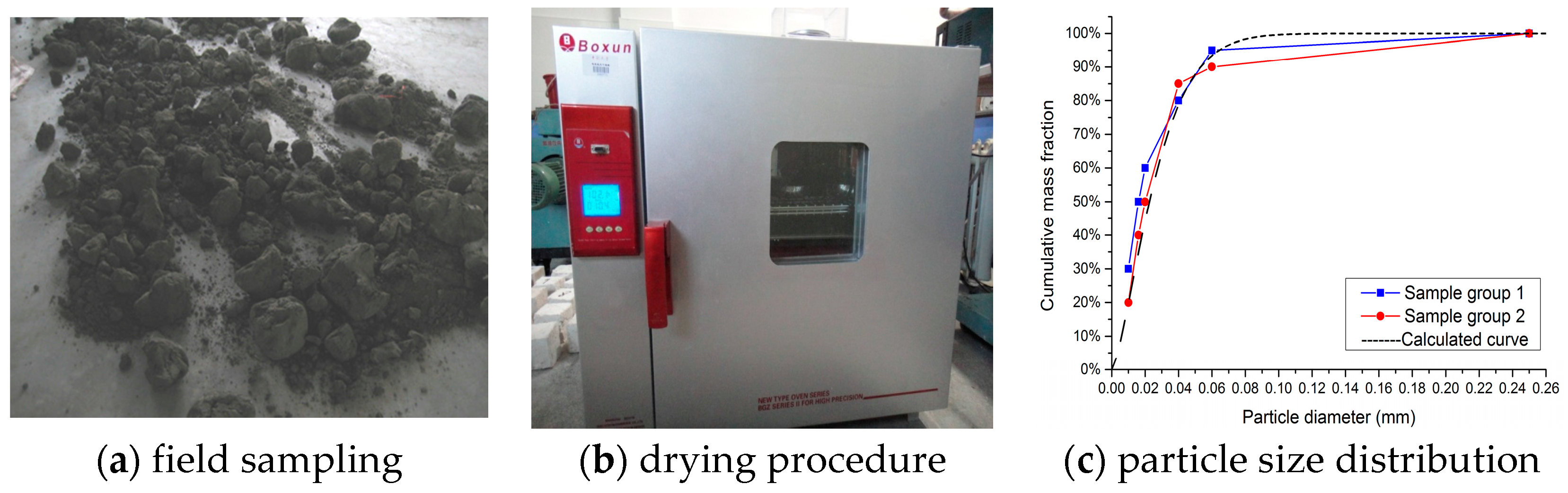
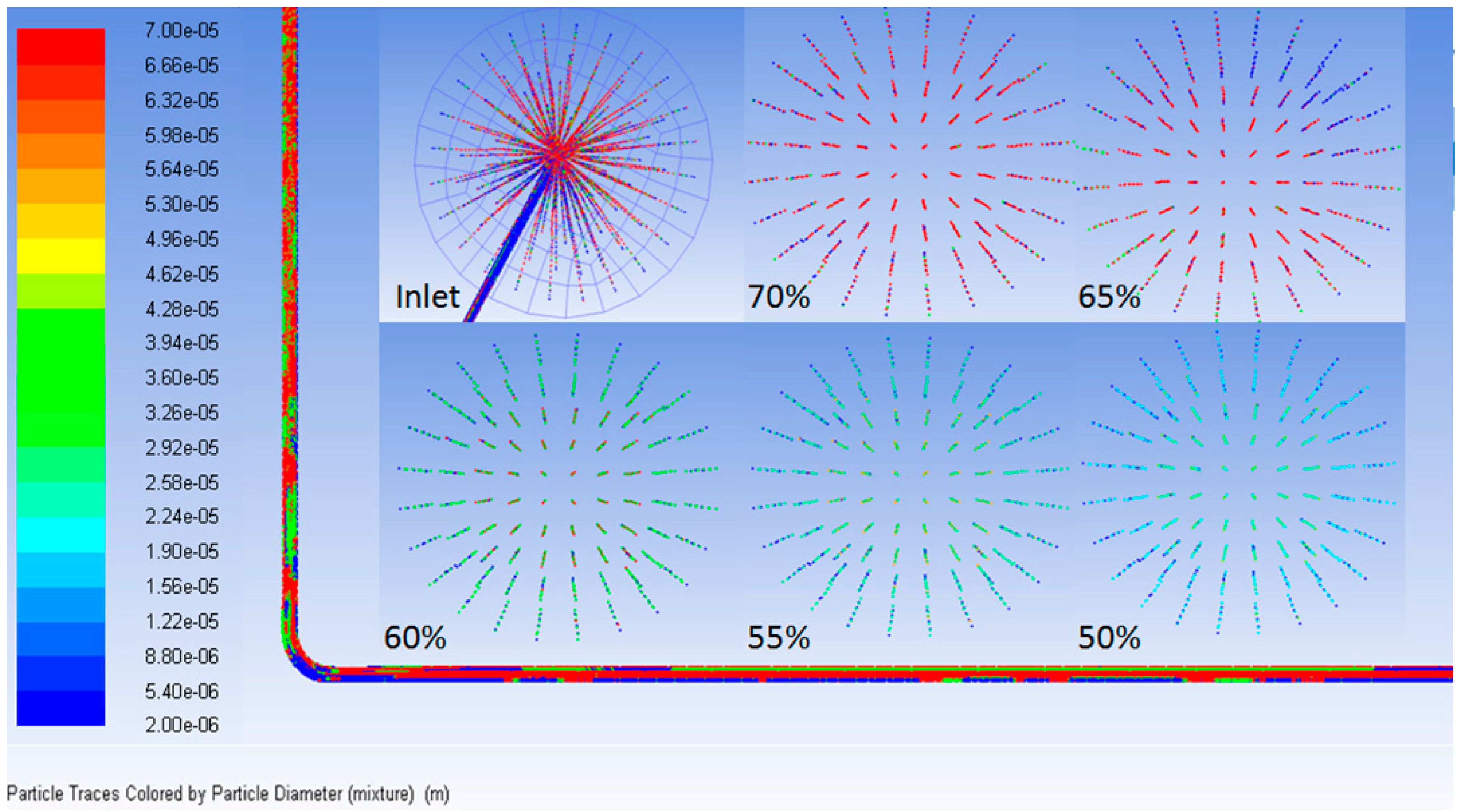
2.3. Particle Flow Distribution
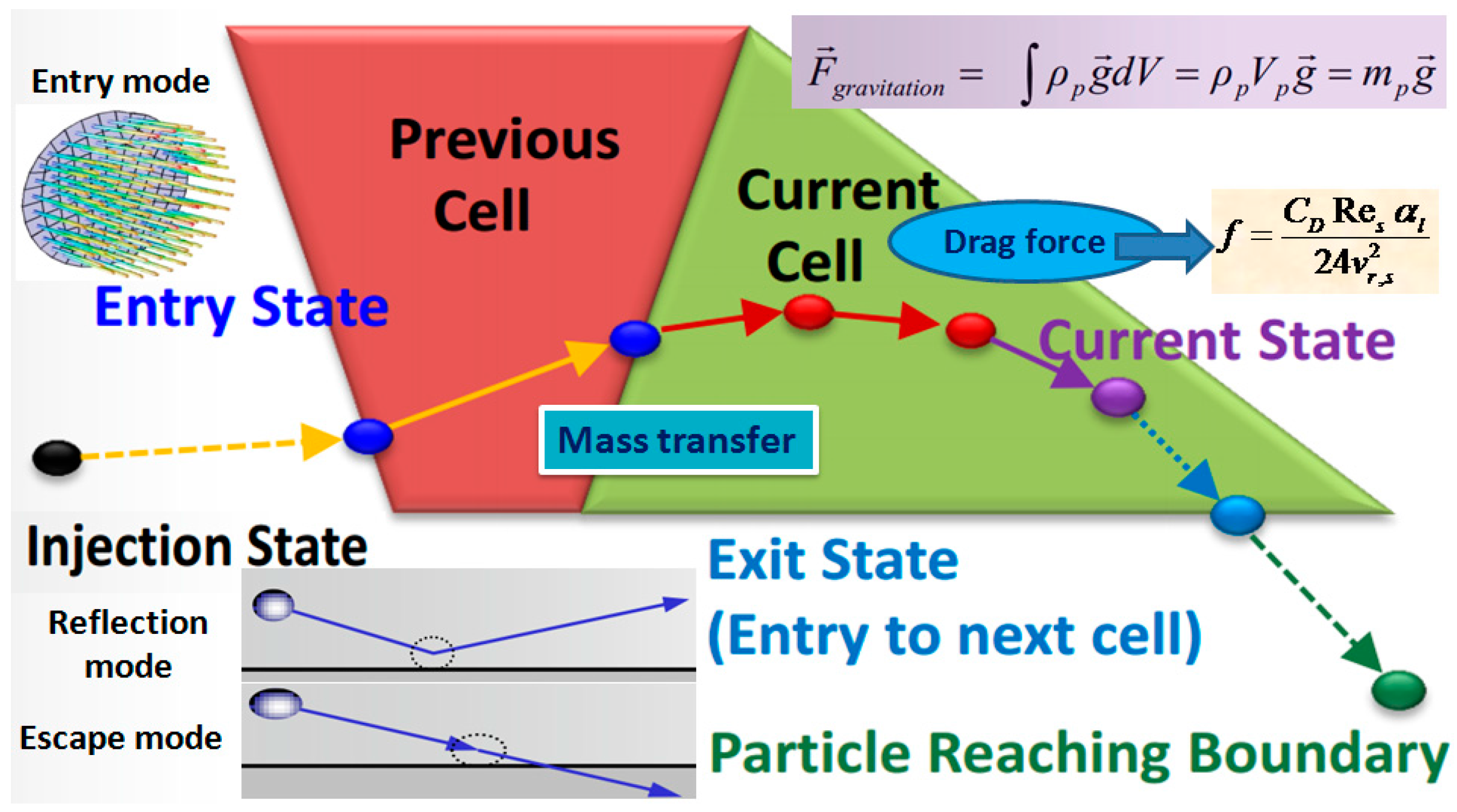
2.4. Calculation Equations
2.5. User-Defined Drag Force Model
thread_l = THREAD_SUB_THREAD(mix_thread, s_col);
thread_s = THREAD_SUB_THREAD(mix_thread, f_col);
                                        ⋮
        if(void_l<=0.85)
        bfac = 0.281632*pow(void_l, 1.28);
        else bfac = pow(void_l, 9.076960);
        vfac = 0.5*(afac-0.06*reyp+sqrt(0.0036*reyp*reyp+0.12*reyp*(2.*bfac-afac)+afac*afac));
        fdrgs = void_l*(pow((0.63*sqrt(reyp)/vfac+4.8*sqrt(vfac)/vfac),2))/24.0;
        k_l_s = (1.-void_l)*rho_s*fdrgs/taup;
                                        ⋮
reyp = rho_l*abs_v*diam2/mu_l;
cd = (24./(reyp+SMALL)) + 5.48*pow((reyp+SMALL),-0.573) + 0.36;
void_l = C_VOF(cell, thread_l);
el = pow(void_l,-2.65);
k_l_s = (3./4.)*(cd*(1.-void_l)*abs_v*rho_l*el)/diam2;
return k_l_s;
3. Results and Discussion
3.1. Mechanism Description
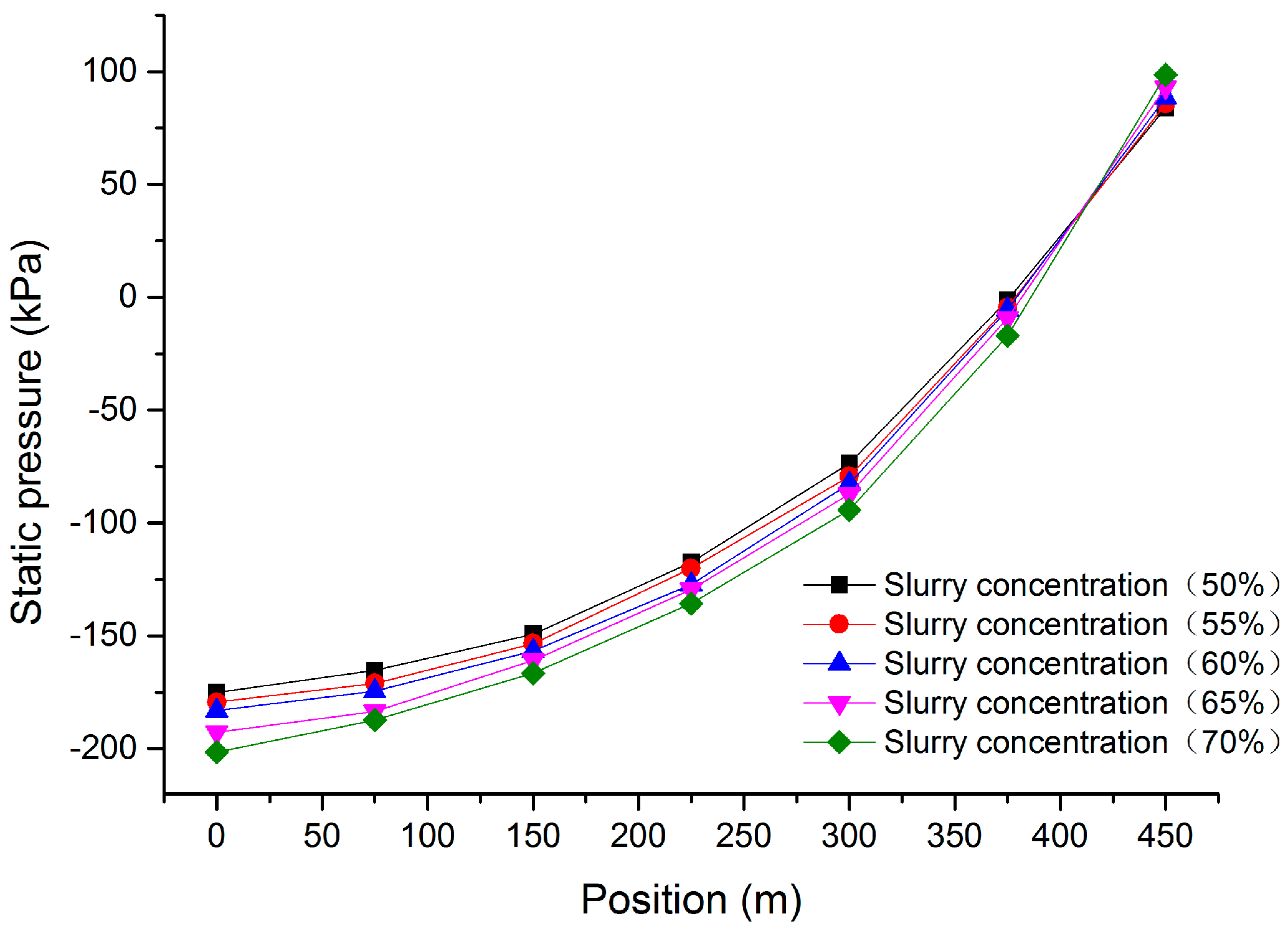
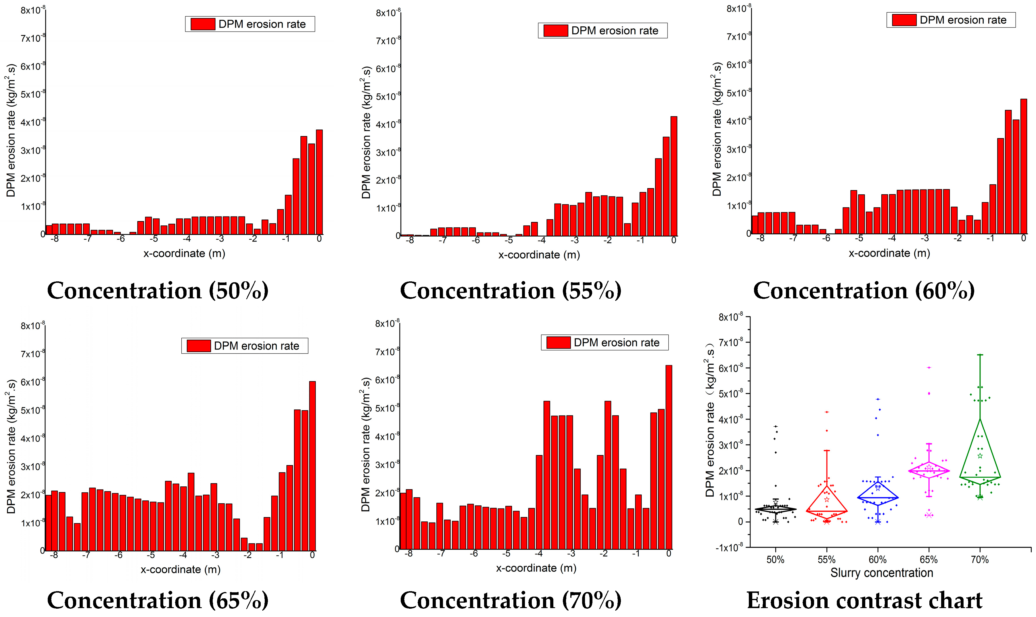
3.2. Concentration Analyses
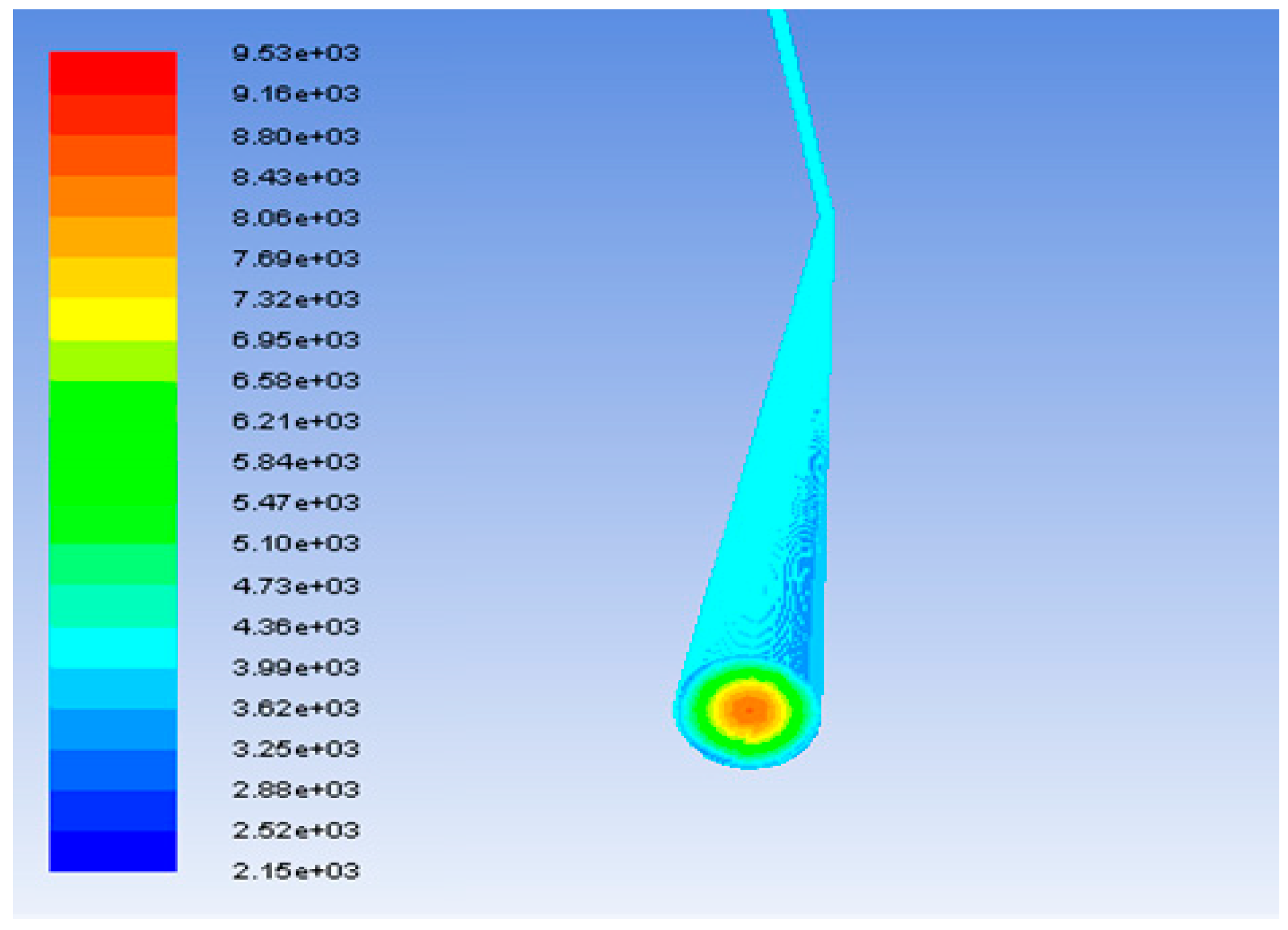
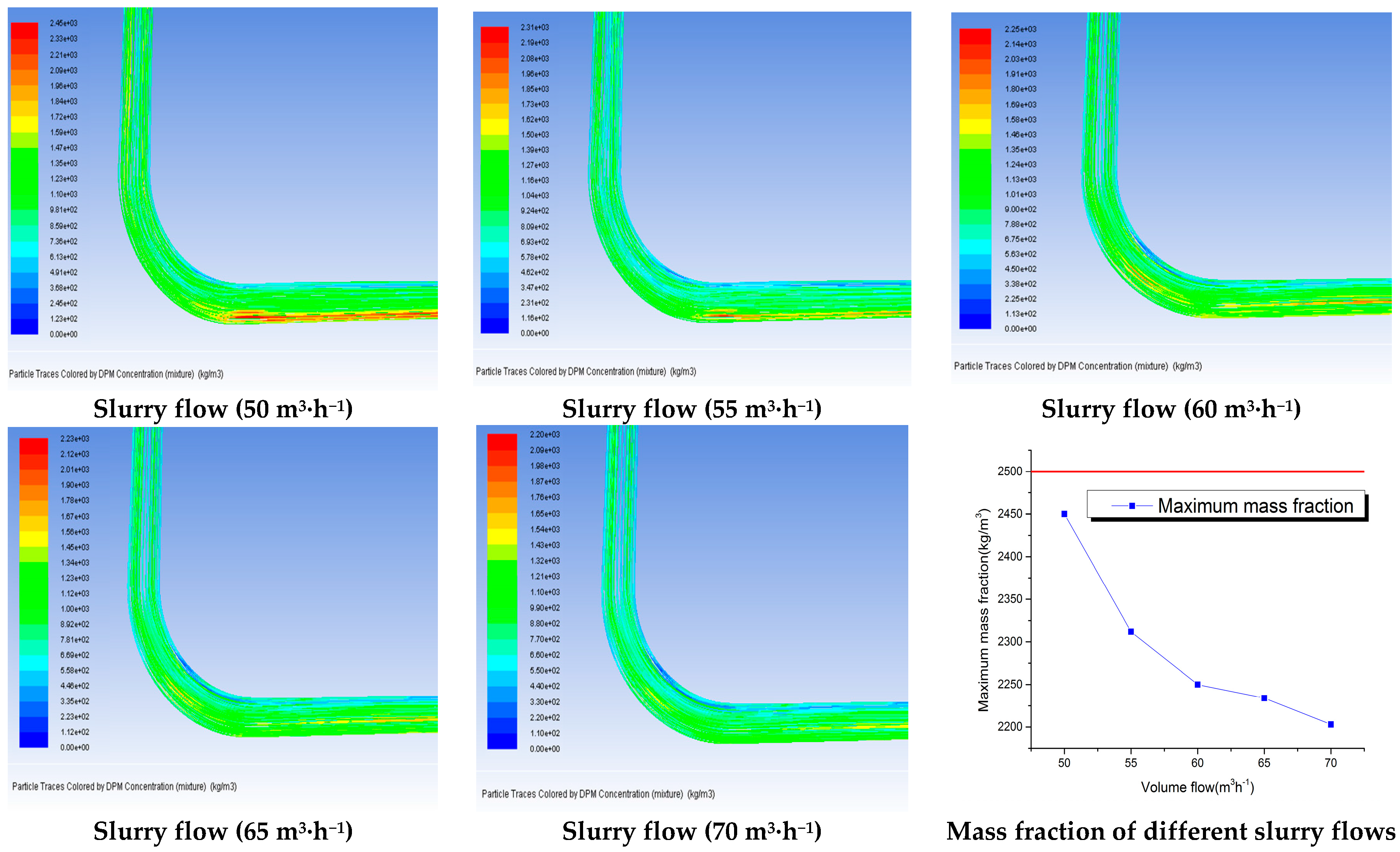
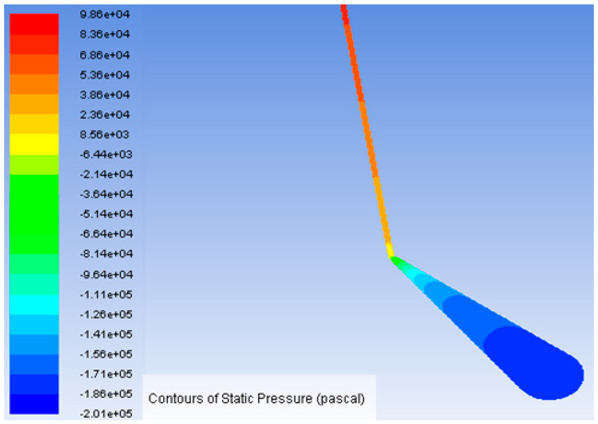
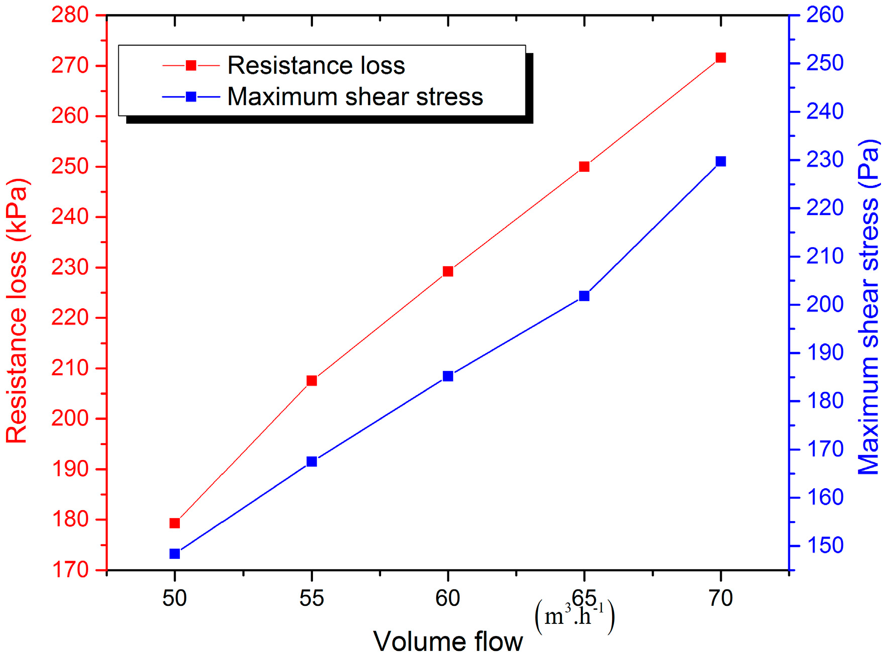
3.3. Slurry Flow Analyses
4. Experimental Verification
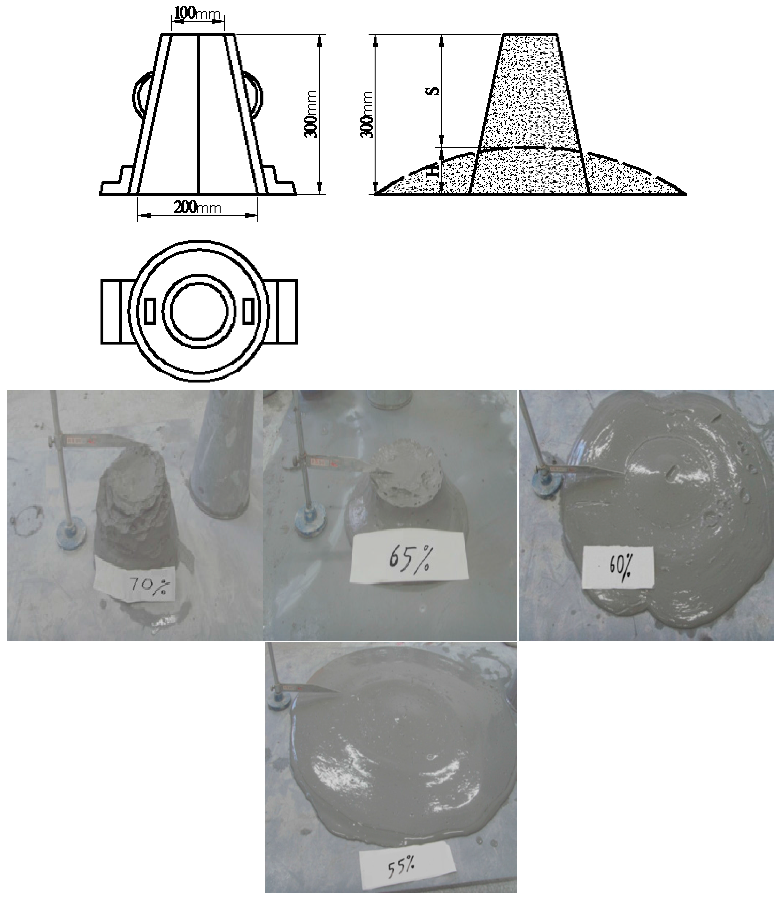
4.1. Slurry Slump Rest
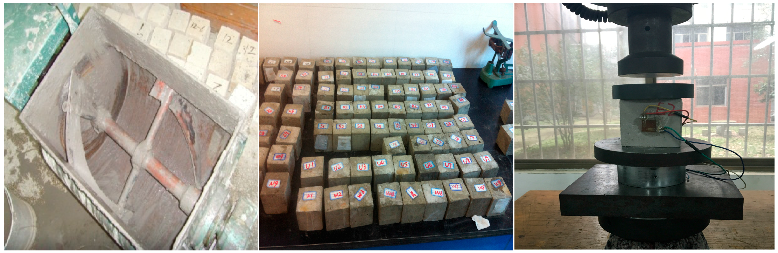
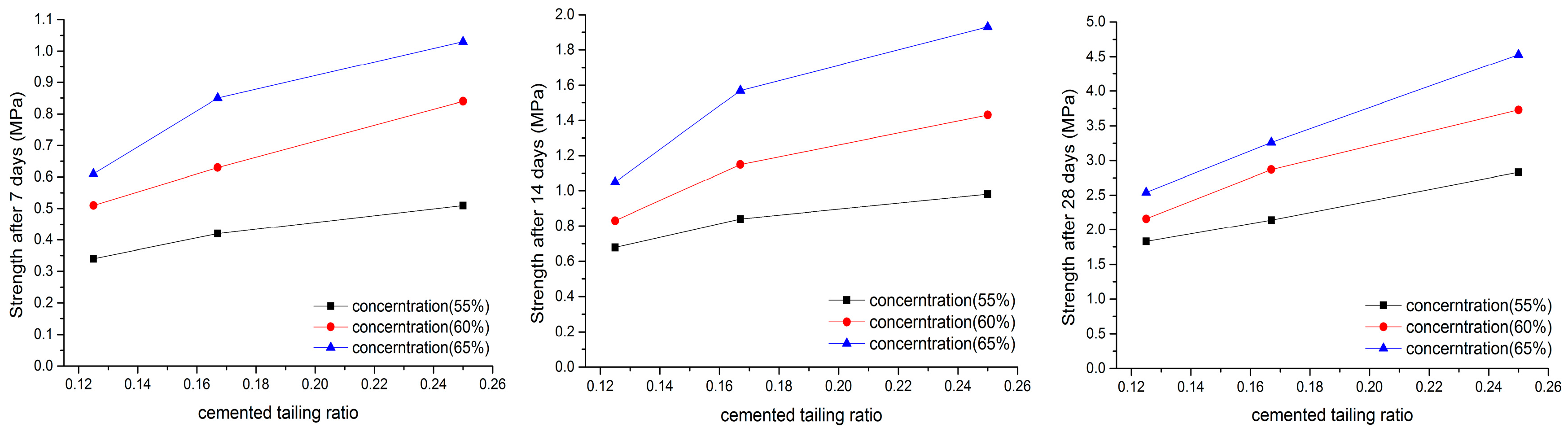
4.2. Backfill Strength Test
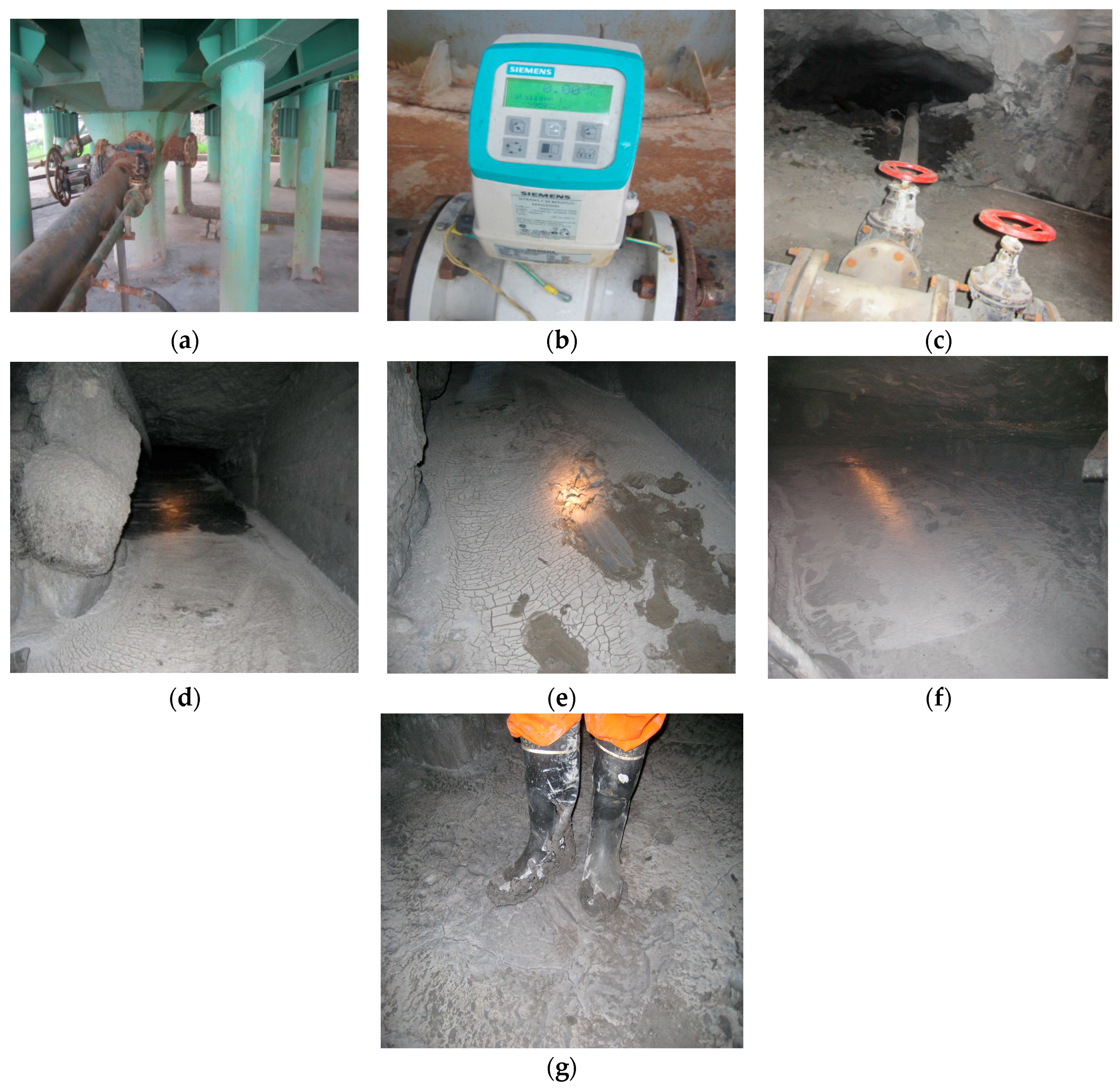
4.3. Industrial Test
5. Summary and Conclusions
- (1)
- In the process of backfilling transportation, pipeline resistance loss and abrasion can be controlled by reducing the flow rate and slurry concentration. Discrete phase analysis results show that reducing transportation parameters may lead to slurry dehydration and low backfill strength. Therefore, transportation parameters need to be controlled within an effective range, in order to realize efficient backfilling.
- (2)
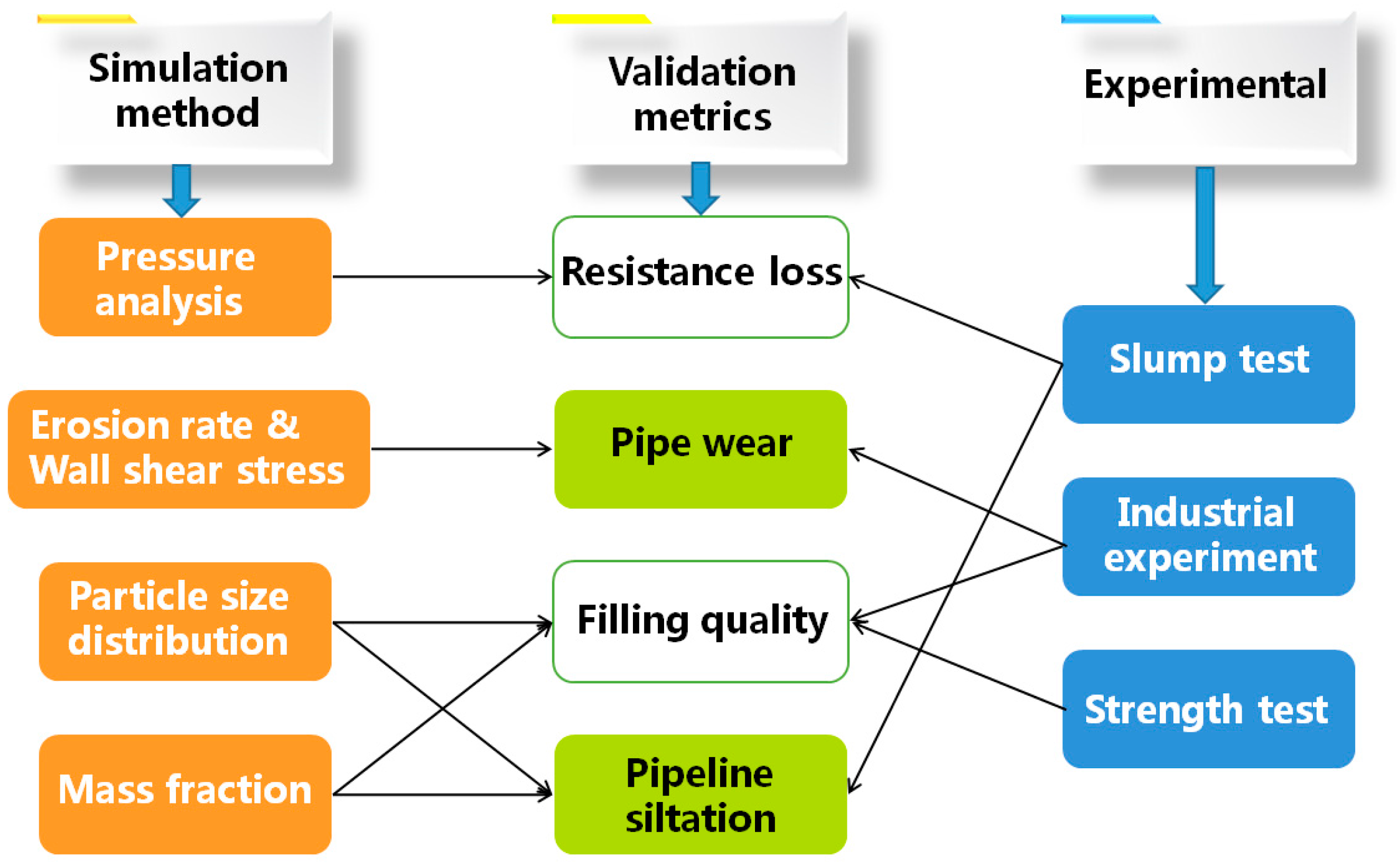
- By application of the CFD-DDPM solid–liquid phase flow model, analyses on multifactor (pressure, particle size distribution, erosion and mass fraction) in two phase mixture flow was conducted. Optimal transportation parameters with a slurry concentration of 60% and volume flow of 55 m3/h were obtained using simulations and experiments. This method can be used by other mining enterprises.
- (3)
- This work is more of a numerical method development, laboratory experiments and industrial experiments were used to verify and calibrate the numerical model. Therefore, a large number of other experiments with different standards have not been carried out. However, in the case of gravity transport, the results and achievements can be accurately used in the design of filling pipeline transport with particle flow characteristics. This method can reduce the dependence on large-scale loop experiments and industrial verification, and also has reference values for oil and gas transportation and water transportation. On the basis of the further development of the software language, the combination of DDPM and experiments is feasible. In order to enhance the fluidity and the filling strength of mining enterprises, the methods of paste filling and coarse aggregate transportation need to be further improved using DDPM methods. Further research is expected to be realized to have more possibilities in backfilling transportation.
Acknowledgments
Author Contributions
Conflicts of Interest
Nomenclature
| G = particle cumulative percentage | [-] | = particle velocity | [m/s] |
| d = particle size | [m] | , = Solid/liquid density | [-] |
| n = distribution index | [-] | = particle acceleration | [m/s2] |
| a = size coefficient | [-] | = gravitational acceleration | [m/s2] |
| d0 = morphological diameter | [m] | = static pressure | [Pa] |
| = density | [kg/m3] | =internal normal stress | [Pa] |
| = laplacian | [-] | = momentum interaction | [kg/m2·s2] |
| = volume fraction | [-] | = shear viscosity | [kg/m·s] |
| , = fluid velocity | [m/s] | = viscous coefficient | [kg/m·s] |
| = interphase mass transfer | [-] | = drag coefficient | [-] |
| = normal unit vector | [-] | = relative reynolds number | [-] |
| , = position vector | [-] | = terminal velocity | [m/s] |
| = moment of inertia | [kg/m2] | = exchange coefficient | [m/s] |
| , = Particle mass | [kg] | = interphase drag force | [N] |
| , =speed vector | [m/s] | , = correction coefficient | [-] |
| = rotation speed vector | [rpm] | = impulse | [kg·m/s] |
References
- Sun, H.H.; Huang, Y.C.; Yang, B.G. Contemporary Cemented Backfilling Technology; Metallurgical Industry Press: Beijing, China, 2002; pp. 113–114. [Google Scholar]
- Sommerfeld, M. Modeling of Particle-Wall Collisions in Confined Gas-Particle Flows. Int. J. Multiph. Flows 1998, 18, 905–926. [Google Scholar] [CrossRef]
- David, H.; Sebastian, A.; Peter, R. Pipe lining abrasion testing for paste backfill operations. Int. J. Multiph. Flows 2009, 22, 1088–1090. [Google Scholar]
- Buffo, A.; Vanni, M.; Marchisio, D.L. Multidimensional population balance model for the simulation of turbulent gas-liquid systems in stirred tank reactors. Chem. Eng. Sci. 2012, 70, 31–44. [Google Scholar] [CrossRef]
- Boger, D.V. Rheology of slurries and environmental impacts in the mining industry. Annu. Rev. Chem. Biomol. Eng. 2013, 4, 239–257. [Google Scholar] [CrossRef] [PubMed]
- David, A.M.; Alastair, D.S. The effects of a highly viscous liquid phase on vertically upward two-phase flow in a pipe. Int. J. Multiph. Flows 2003, 29, 1523–1538. [Google Scholar]
- Zeng, M.; Xu, Z.Q.; Huangfu, J.H.; Liu, J.T.; Zhang, R.Z. Two-phase flow numerical simulation of jet flotation column. J. China Coal Soc. 2008, 33, 795–798. [Google Scholar]
- Dykas, S.; Wróblewski, W. Single-and two-fluid models for steam condensing flow modeling. Int. J. Multiph. Flows 2011, 37, 1245–1253. [Google Scholar] [CrossRef]
- Thiruvengadam, M.; Zheng, Y.; Tien, J.C. DPM simulation in an underground entry: Comparison between particle and species models. Int. J. Min. Sci. Technol. 2016, 26, 487–494. [Google Scholar] [CrossRef]
- Adamczyk, W.P.; Klimanek, A.; Białecki, R.A.; Węcel, G.; Kozołub, P.; Czakiert, T. Comparison of the standard Euler-Euler and hybrid Euler-Lagrange approaches for modeling particle transport in a pilot-scale circulating fluidized bed. Particuology 2014, 15, 129–137. [Google Scholar] [CrossRef]
- Ni, C.J.; Lu, G.C.; Zhang, Q.D.; Jing, T.; Wu, J.J.; Yang, L.L.; Wu, Q.F. Influence of core box vents distribution on flow dynamics of core shooting process based on experiment and numerical simulation. China Foundry 2016, 13, 22–29. [Google Scholar] [CrossRef]
- Angst, R.; Kraume, M. Experimental investigations of stirred solid/liquid systems in three different scales: Particle distribution and power consumption. Chem. Eng. Sci. 2006, 61, 2864–2870. [Google Scholar] [CrossRef]
- Wang, F.; Mao, Z.; Wang, Y. Measurement of phase holdups in liquid-liquid-solid three-phase stirred tanks and CFD simulation. Chem. Eng. Sci. 2006, 61, 7535–7550. [Google Scholar] [CrossRef]
- Lee, S.H.; Kim, H.J.; Sakai, E.; Daimon, M. Effect of particle size distribution of fly ash-cement system on the fluidity of cement pastes. Cem. Concr. Res. 2003, 33, 763–769. [Google Scholar] [CrossRef]
- González-Tello, P.; Camacho, F.; Vicaria, J.M.; González, P.A. A modified Nukiyama-Tanasaw a distribution function and a Rosin–Rammler model for the particle-size-distribution analysis. Powder Technol. 2008, 186, 278–281. [Google Scholar] [CrossRef]
- Foerster, S.F.; Louge, M.Y.; Chang, H.; Allia, K. Measurements of the Collision Properties of Small Spheres. Phys. Fluids 1994, 6, 1108. [Google Scholar] [CrossRef]
- Dallavalle, J.M. Micromeritics; Pitman Publishing Corpration: New York, NY, USA, 1948. [Google Scholar]
- Syamlal, M. The Particle-Particle Drag Term in a Multiparticle Model of Fluidization; National Technical Information Service: Springfield, VA, USA, 1987; pp. 1353–2373. [Google Scholar]
- Richardson, J.R.; Zaki, W.N. Sedimentation and Fluidization: Part I. Trans. Inst. Chem. Eng. 1954, 32, 35–53. [Google Scholar]
- Garside, J.; Al-Dibouni, M.R. Velocity-Voidage Relationships for Fluidization and Sedimentation. Ind. Eng. Chem. Process Des. Dev. 1977, 16, 206–214. [Google Scholar] [CrossRef]
- Wu, D.; Cai, S.J.; Yang, W.; Wang, W.X.; Wang, Z. Simulation and experiment of backfilling pipeline transportation of solid-liquid two-phase flow based on CFD. Chin. J. Nonferr. Met. 2012, 22, 2133–2140. [Google Scholar]
- Huser, A.; Kvernvold, O. Prediction of sand erosion in process and pipe components. In Proceedings of the 1st North American Conference on Multiphase Technology, Banff, AB, Canada, 10–11 June 1998; Volume 31, p. 217.


| Slurry Concentration (%) | Inlet Pressure (kPa) | Outlet Pressure (kPa) | Resistance Loss (kPa) |
|---|---|---|---|
| 70 | 98.6 | −201.5 | 300.1 |
| 65 | 93.2 | −192.7 | 285.9 |
| 60 | 88.5 | −183.1 | 271.6 |
| 55 | 85.7 | −179.3 | 265.0 |
| 50 | 83.8 | −175.1 | 258.9 |
| Slurry Concentration (%) | Particle Size Range (mm) | Weighted Average Value (mm) |
|---|---|---|
| 70 | 0.011–0.25 | 0.059 |
| 65 | 0.007–0.17 | 0.045 |
| 60 | 0.002–0.11 | 0.027 |
| 55 | 0.002–0.066 | 0.021 |
| 50 | 0.002–0.049 | 0.018 |
| Volume Flow (m3·h−1) | Inlet Pressure (kPa) | Outlet Pressure (kPa) | Resistance Loss (kPa) |
|---|---|---|---|
| 70 | 88.5 | −183.1 | 271.6 |
| 65 | 79.6 | −170.4 | 250.0 |
| 60 | 70.9 | −158.3 | 229.2 |
| 55 | 61.3 | −146.2 | 207.5 |
| 50 | 53.4 | −125.9 | 179.3 |
| Slurry Concentration (%) | 50 | 55 | 60 | 65 | 70 |
|---|---|---|---|---|---|
| Slump/cm | - | 27.6 | 22.1 | 16.8 | 10.1 |
© 2017 by the authors; licensee MDPI, Basel, Switzerland. This article is an open access article distributed under the terms and conditions of the Creative Commons Attribution (CC-BY) license (http://creativecommons.org/licenses/by/4.0/).
Share and Cite
Zhou, K.-p.; Gao, R.; Gao, F. Particle Flow Characteristics and Transportation Optimization of Superfine Unclassified Backfilling. Minerals 2017, 7, 6. https://doi.org/10.3390/min7010006
Zhou K-p, Gao R, Gao F. Particle Flow Characteristics and Transportation Optimization of Superfine Unclassified Backfilling. Minerals. 2017; 7(1):6. https://doi.org/10.3390/min7010006
Chicago/Turabian StyleZhou, Ke-ping, Rugao Gao, and Feng Gao. 2017. "Particle Flow Characteristics and Transportation Optimization of Superfine Unclassified Backfilling" Minerals 7, no. 1: 6. https://doi.org/10.3390/min7010006
APA StyleZhou, K.-p., Gao, R., & Gao, F. (2017). Particle Flow Characteristics and Transportation Optimization of Superfine Unclassified Backfilling. Minerals, 7(1), 6. https://doi.org/10.3390/min7010006