Article

Geometallurgical Modeling of Influence of Mineral Composition of Sulfide Copper Ore (Southwest Poland) on Enrichment Selectivity

by
Magdalena Duchnowska
* and
Alicja Bakalarz
Department of Mining, Faculty of Geoengineering, Mining and Geology, Wroclaw University of Science and Technology, Wybrzeże Wyspiańskiego 27, 50-370 Wrocław, Poland
*
Author to whom correspondence should be addressed.
Minerals 2025, 15(4), 432; https://doi.org/10.3390/min15040432
Submission received: 19 March 2025 / Revised: 13 April 2025 / Accepted: 18 April 2025 / Published: 20 April 2025
(This article belongs to the Section Mineral Processing and Extractive Metallurgy)

Abstract

The aim of this research was to determine a relationship that would allow the results of the enrichment process to be predicted from the mineral and chemical composition of the of sedimentary copper ores present in the Fore-Sudetic monocline (SW Poland). A series of laboratory flotation tests of feeds with different lithological compositions of copper ores (sandstone, dolomitic, and shale) as well as detailed chemical and mineral analyses of feeds and flotation products were carried out. Based on the obtained results, enrichment selectivity indicators were determined and used in modeling. Among the methods of statistical dimensional analysis, multivariate correlation was used for modeling. The result of modeling was the equation that allowed the prediction of the results of the copper ore enrichment process from the contents of the main rock-forming minerals (clays/micas and carbonates) and copper in the feed. The equation is highly precise and can be used to predict the results of copper ore enrichment on the basis of the mineral and chemical compositions of the feed (correlation coefficient of 0.78). The proposed equations may be employed in an industrial process to determine its metallurgical result in the case of variable ore lithology.

1. Introduction

Geometallurgy is an interdisciplinary approach in which geological, metallurgical, environmental, and economic information is combined in order to design and manage mining production, with a focus on the final metallurgical product of ore treatment [1,2,3,4]. Modern metallurgy aims at integrating earth sciences with mineral and mining engineering. By combining the geological, mineralogical, technological, and economic information related to the processing of mineral raw materials, it is possible to determine the value of the deposit, as well as rational extraction methods and treatment technologies, and to evaluate the technical and operational risk of the project, thus facilitating the development of an effective mine [4,5,6]. To a lesser extent, geometallurgical modeling aided by process mineralogy can be used to evaluate the ongoing performance of process systems and can also contribute to solving current problems in the technology scheme of mineral processing plants [7,8]. As an integrated multidisciplinary approach, geometallurgy identifies the data required in a deposit mining model, which is necessary for the economically optimal management of a deposit. These elements form the basis for adopting optimal technological parameters and for designing mineral processing systems that can be adjusted in near real time to the variability in the processed ore [5,9].
The main elements of geometallurgical modeling include preliminary geological surveys used for preparing a geological sampling plan, the sampling process, technological laboratory tests, developing a model for the transition from the laboratory scale to the industrial scale, a technological test on the industrial scale, and a transition model allowing predictions of industrial results on the basis of the laboratory data or adjustments of the existing systems to the modeled results. Depending on the conditions, such elements may comprise 3–8 stages [1,10,11,12]. Figure 1 presents the main elements of the geometallurgical modeling process based on Lamberg (2011) [11] and Lund et al. (2015) [13].
In the geometallurgical approach, the ore deposit is tested with the aim of identifying variabilities within the limits of the deposit and determining the spatial geometallurgical domains that show different reactions to the steps involved in mineral processing. By employing such geometallurgical domains in designing ore enrichment technology and in defining an ore extraction schedule plan, it is possible to respond flexibly to feed variability in cases when different ore types are sent to the processing plant. The basic parameters used in geometallurgical modeling include geological data (blocks, parts, deposit domains of particular metallurgical properties), which are subsequently correlated with the results of metallurgical tests (enrichment) obtained from laboratory and industrial experiments [2,11,13,14,15]. The model resulting from the data analysis may serve as a basis for the management of mining production, as well as mineral and metallurgical processing.
The geometallurgical approach is most frequently used in the case of large deposits having long-term extraction plans. It is also becoming an important element in cases of small deposits with a complicated geological structure and of secondary deposits [16,17,18,19]. As rich deposits of metallic raw materials are becoming depleted, mining companies are forced to focus on low-grade deposits having complex geological and mineralogical characteristics. In such cases, a broad dataset and geometallurgical correlations allow the mining and processing operations to be optimally designed [5,20].
Analyses of mining resources are typically performed with conventional techniques, e.g., univariate statistical tools (geostatistics). In the case of constructing geometallurgical models, estimations of the process parameters are aided by a more useful tool: multivariate statistics [21,22].
The basic methods for defining statistical multivariate relationships include generalized correlation, regression and variance analyses, principal component analysis, classification, factor analysis, and discriminatory analysis [23]. One of the primary elements in multivariate analysis is the investigation of the correlations among variables. In the case of data describing the effectiveness of the laboratory enrichment of selected feed, the analysis of the results obtained from a multivariate correlation equation may become a basis for predicting industrial results on the condition that the analysis rests on properly defined real confidences for the selected independent variables [24].
Strategic decisions regarding the development of mineral deposits are biased with geological uncertainties typically due to the limited number of geological samples. The long-term extraction plans typically used in industry can successfully address this geological variability, but they neither describe how a mineral processing plant should react to the variability in the ore in the feed nor predict the result of the ore enrichment processes [20]. Therefore, the next logical step is to expand long-term extraction planning methods with geometallurgical modeling, which combines geological variability with the metallurgical effectiveness of the beneficiation process [1].
The basic data used in geometallurgical modeling are the chemical and mineralogical properties of the ores; also applicable is the information that determines the main metallurgical indicators of the enrichment processes. The main parameters used in geometallurgical modeling include comminution indicators (Bond Work Index, P80) and enrichment indicators (recovery, parameters of flotation kinetics and selectivity, etc.) [5,10,15,20].
Quantitative modeling methods are the basis for the precise understanding and identification of the processes. In most cases, the aim is to model the deposit on the basis of the fundamental laws describing physical phenomena, for instance, the mass conservation law. In the case of describing the enrichment process of the copper ore from the Fore-Sudetic monocline, the models primarily describe the processing of granular materials [25] or the optimization of technological systems in mineral processing plants [26,27], but they do not incorporate the lithology or mineralogy of the processed ore.

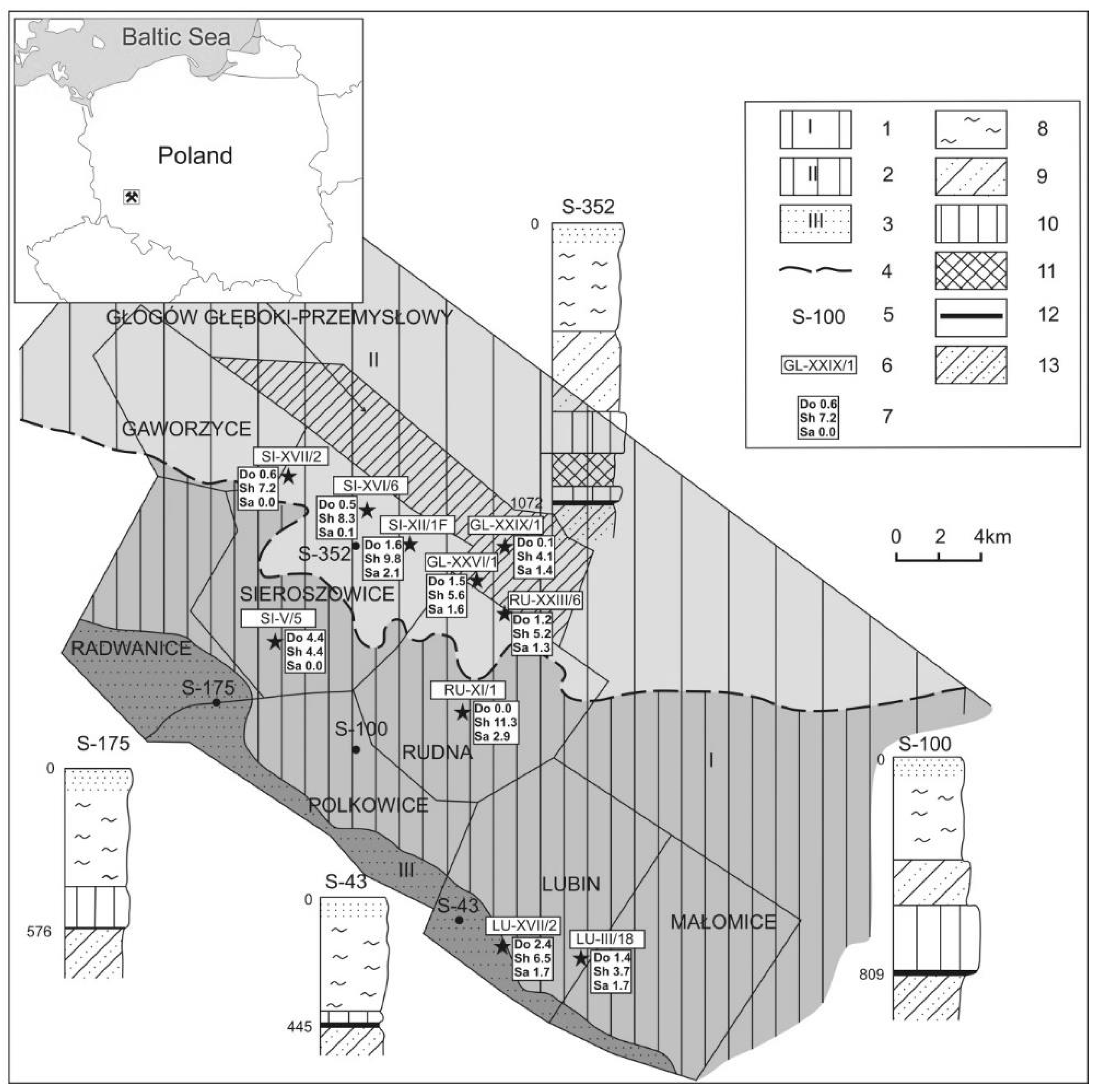
Characteristics of Stratiform Copper Ore from Legnica-Glogow Copper Basin (LGCB)

The strata-bound deposit in the Legnica-Glogow Copper Basin (LGCB) is a part of the Central European Copperbelt, characterized by polymetallic mineralization that is referred to as Kupferschiefer [28]. This is the largest sediment-hosted strata-bound copper deposit in Europe and has been mined for over 60 years by the Mining-Smelting Complex KGHM Polska Miedz SA, which is the largest producer of primary copper in Europe and one of the largest producers of silver in the world [29,30]. In Table 1, the mass balance of the KGHM Polska Miedz SA production for 2022 is presented. In addition to copper and silver, the ore also contains significant amounts of Pb, Zn, Ni, Co, and Au [31,32]. The ore consists of three different lithology types, sandstone, dolomitic, and shale, which have markedly different chemical and mineralogical compositions, physical properties, and floatabilities [33]. These three different lithology types are mined together and processed in the mixture. Sandstone is the easiest to upgrade but the copper grade is low (0.8%–1.5%). The dolomitic ore is fairly upgradeable and contains 0.5%–1.9% copper.
The richest in copper and other precious metals but poorly upgradeable is clayey-dolomitic-bituminous black shale. The content of copper in this lithology type ranges from 2.8 to 8.7%. The main copper sulfides occurring in all three types of lithology are chalcocite, bornite, covellite, chalcopyrite, digenite, and, less frequently, djurleite, tennantite, tetrahedrite, and enargite. In addition to copper, these ores contain pyrite, marcasite, galena, and sphalerite [34,35,36].
Kaczmarek et al. [36] distinguished 16 specific lithology types, identified with the use of macroscopic methods, in samples taken from mining excavations. There were four types of sandstones, three types of shales, eight types of dolomitics, and anhydrite/rock salt. The detailed lithological data were of great practical importance and were used for the geologic evaluation of the deposit as well as mining production planning [36]. The geological data acquired by geologists and the results of flotation tests at KGHM processing plants allowed the identification of three types of shales: organic shale, silty shale, and dolomitic shale. The engineers in the processing plant referred to the other ore types as sandstone and carbonate ores and did not further classify their lithologies.
The technological properties of the copper ore from the LGCB deposit are specific and not frequently encountered in other copper resources worldwide. The sedimentary characteristics of the deposit, as well as the complex petrographic and mineral composition of the ore, are the main reasons for the technological problems that have already occurred during the mineral processing and the smelting stages. The presence of three lithological types in varying proportions necessitates the implementation of complicated technological enrichment systems and is an obstacle to maintaining high recovery and contents of precious metal in final concentrates, which decrease systematically over time. The most prominent indication of this problem can be found when analyzing the metal losses in flotation tailings [37,38,39].
In the mining and processing operations of KGHM Polska Miedz SA, the shale layer is of particular importance, as it determines the total content of the useful components in the deposit [40,41,42]. Therefore, it is of high economic value. According to Kijewski and Leszczynski (2010) [34], depending on the region of the deposit, the shale layer holds 30 to 45% of the entire copper content, which means that of the three lithology types of ore, shale ore has the highest content of copper. In addition, this ore is rich in other associated metals within the ore, such as Ag, Co, Mo, Ni, Zn, Pb, and Au [43,44,45]. This layer represents approximately 11% of the ore mass in the industrial resources of the LGCB deposit. Shale ore has the lowest floatability of all three types of copper ore. The content of this type in the feed has a major impact on the effectiveness of the enrichment processes. As the content of shale ore in the flotation feed increases, it becomes increasingly difficult to maintain the required recoveries and concentrate quality [39,46]. The content of shale ore in the feed to processing plants has a major impact on the efficiency of the beneficiation process. The mineral and chemical compositions of the shale ore have the greatest impact on the effect of geometallurgical modeling and are the main bases on which any issues develop.
The geometallurgical modeling of the copper ore deposit in the Fore-Sudetic monocline has been started by constructing a 3D geological model [47,48]. Two structural models have been constructed. The first one was based on the general classification of lithology types of ore (sandstone, dolomitic and shale). The second was based on a detailed classification (16 types of lithology). The detailed model allowed the mining processes to be optimized, particularly with respect to the estimations of the main minerals in the ore, and the general model allowed estimations of geological resources. The model allowed assessments of the quality parameters of the deposit based on the lithological composition [36]. However, the resulting model focused solely on geological data, without considering the evaluation of the floatability of the different lithological varieties of ore and its effect on the economic effect of the enrichment process.
The general geological model served as a basis for identifying locations in which samples for enrichment were collected. These samples were subjected to detailed chemical and mineralogical analyses. Both pure lithological ores samples and their mixtures were tested for their upgradability characteristics [49]. The next stage of this study was the determination of a geometallurgical model allowing the metallurgical effectiveness of the enrichment process to be approximated on the basis of the mineral composition of individual lithologies in the processed copper ore. The metallurgical effectiveness of the enrichment process was identified with the parameters of the multivariate correlation equation, which allowed predictions of enrichment results to be made by analyzing the contents of the main rock-forming minerals and copper in the feed in the enrichment process. The equation is expected to provide information on technological results without the need to perform time- and cost-intensive laboratory flotation tests.

2. Materials and Methods

Generally, the research methodology comprised two parts: a series of laboratory flotation and analytical analyses performed on the basis of the laboratory part results. The tests included the following actions:
  • Sampling and collecting representative samples for the comminution test—preparation of averaged mixtures of pure lithological types and their comminution for the flotation process (wet grinding);
  • Conducting 120 flotation tests;
  • Performing chemical and mineralogical analyses of the feed and of the enrichment product;
  • Identifying parameters affecting enrichment process, together with the effectiveness of the enrichment process;
  • Developing the geometallurgical model’s equation and verifying it for consistency with the actual data.

2.1. Sampling

Copper ore samples for testing were taken by the KGHM geological staff using a 3D geological model of the deposit. The samples for the flotation tests were collected from 10 locations on the deposit of the Fore-Sudetic monocline, as shown in Figure 2.
Samples of shale, sandstone, and carbonate ore were taken separately from each location (total 30 samples were taken from the deposit to test). The sampling locations are indicated in Figure 2 with the symbol numbered 6 in the legend (these symbols indicate the mining division from which the samples were collected).
The samples were crushed in a laboratory jaw crusher (LAB-02-130, EKO-LAB, Brzesko, Poland). After each crushing, the ore was sieved through a sieve with a mesh of 1 mm, and then the upper product of the sieving was crushed again. The operations were repeated until the whole sample was within the grain class of less than 1 mm; the whole crushing was completed within up to 6 cycles. Then, sampling was carried out for chemical and mineral analyses from each of the 30 lithological types of copper ore. Chemical analyses of the ore samples (determination of copper content) were carried out at a certified laboratory in the Centre of Analytical Chemistry of Lukasiewicz Research Network—Institute of Non-Ferrous Metals in Gliwice (Poland). Copper was determined by iodometric titration. Mineral analyses of the ores were performed at the Structures and Materials Research Laboratory of Lukasiewicz Research Network—PORT Polish Center for Technology Development in Wroclaw (Poland). The analyses were conducted using an automated mineral analysis system, QEMSCAN®, with a Quanta 650 FEG microscope produced by FEI Company (Hillsboro, OR, United States). The detailed methodology of these analyses was previously presented [50]. For each ore sample, the same surface consisting of 25 squares, randomly selected using software, with a side of 1500 μm was analyzed. The measurement step was established at 3 μm. The threshold number of pulses counted by the EDS detector for each point was set to 3 000 in order to obtain more reliable data. The results of the chemical and mineral analyses of the ores are shown in Table 2. Some of the data in this table (copper contents in lithological types) are also presented in Figure 2 (symbol 7 in the legend).
Figure 2. Locations of sample collection and copper grade characteristics for the three lithology types presented on a map of documented LGCB deposits (own study based on the map by Kijewski and Lis, 1996 [51]). 1—Central area, 2—northern area, 3—southern area, 4—southern limit of rock-salt, 5—geotechnical model of the rock mass system, 6—locations of sample collection, 7—copper grade (in %) in the three lithologies (Do—dolomite, Sh—shale, Sa—sandstone), 8—detached and cohesive rocks, 9—low-strength rocks, 10—high-strength cohesive rocks, 11—rheological layer, 12—copper ore deposit, 13—cohesive rocks.
Minerals 15 00432 g002

2.2. Feed Sample Preparation for Flotation

After the samples were crushed, the samples from different lithology types were mixed in proportions shown in Table 3. For each of the 10 sample acquisition locations, 12 lithological mixtures of shale, dolomitic and sandstone ore were prepared (a total of 120 samples). The mixtures simulate the probable lithological compositions of the material planned for extraction [39].
The prepared mixtures of the copper ore lithology types were comminuted in a laboratory ball mill with a capacity of 2.5 dm3. The wet grinding procedure was performed by filling the mill with balls (up to approximately 40% of its capacity) with 800 g of the prepared ore mixture and 0.5 dm3 of processing water. The flotation tests directly followed the sample comminution. The flotation feed samples were characterized by a grain size below 0.2 mm, with a grain size of P50 for the tested samples of about 0.03 mm.

2.3. Flotation Test Methodology

The tests were performed with the standard Dell flotation methodology for multiple experiments [35]. The individual experiment consisted of rougher flotation followed by two cleaning steps. During rougher and cleaning flotation, two products each were obtained: the froth product, which was the feed for the next flotation stage, and the chamber product, which was a tailing or semi-product. The last cleaning flotation, three froth products (concentrates, collected after different flotation times) and a semi-product as a chamber product, were received. Finally, 6 products were obtained from each flotation. The pH of the suspension was neutral (between 7.5 and 8.5).
The flotation tests were performed in a Denver D12 laboratory flotation machine in 2.5 and 1.5 dm3 flotation cells in the rougher and cleaning flotation stages, respectively. During the rougher flotation, the concentration of solid particles in the flotation cell was 300 g/dm3 (density of approx. 1 215 g/dm3). During the flotation experiment, the impeller speed and the air rate were defined as required.
During the experiments, flotation reagents were added at the beginning of the rougher flotation, after the mixture was agitated in the cell without air access. The flotation collector portion was divided into two parts: 60% of the amount was added at the beginning of the rougher flotation and 40% after 5 min of the flotation. The frother was added once at the beginning of the rougher flotation. The mixing time of the flotation slurry with reagents without adding air was about three minutes. The flotation collector was a mixture of sodium ethyl xanthate and sodium isobutyl xanthate mixed in a ratio of 50:50 and added at 100 g/t. The frother was a mixture of polyethylene glycols (Nasfroth) and added at 20 g/t. Industrial flotation reagents were added to the process; concentrated reagents were taken from the concentrator plant.
A total of 120 flotation tests were performed: 12 tests for each sampling location of the pure lithological types. Two products were obtained from each flotation: concentrates and tailings. To calculate the qualitative–quantitative balances, the yields of the flotation products and the copper contents were determined (a total of 240 samples). Copper assays, similar to the flotation feed samples, were conducted by iodometric titration at an accredited laboratory. On the basis of the yields and copper contents of the feeds and flotation products, the recoveries of copper in the concentrates were determined.

2.4. Metallurgical Investigation and Model Development

The effectiveness of the enrichment process as a geometallurgical target function was measured with the use of an enrichment selectivity indicator a, which was calculated from the parameters describing the enrichment curves. Fuerstenau curves (recovery–recovery) describe the relationship between the copper recovery in the concentrate and the recovery of the remaining components in the tailings [52]. For each mixture sample, copper enrichment selectivity indicators were identified according to Equation (1):
a = ε ε r 100 ε ε r
where a is the enrichment selectivity indicator for the Fuerstenau curve symmetrical to the diagonal, ε is the copper recovery in the concentrate, and εr is the recovery of the remaining components in the tailings.
The selectivity indicator a is a parameter produced by the mathematical transformation of the recoveries of the useful minerals in the concentrate and of the remaining components in the tailings, which allows the single-parameter evaluation of the enrichment process results. The higher its value, the lower the enrichment selectivity of the analyzed component [52]. For example, a mixture with a selectivity indicator of 101 shows higher copper enrichment selectivity than a mixture with a selectivity indicator of, e.g., 104, which indicates lower enrichment effectiveness. The selectivity indicator allows a single-parameter evaluation of the effectiveness of the enrichment process and the prediction of the enrichment curves within the entire range of the enrichment parameters. It also has low self-similarity with the primitive enrichment parameters. The degree of self-similarity of parameters is defined by the degree to which one parameter is part of another. This is due to the development of the graphical interpretation of enrichment parameters in enrichment curve systems and their self-similarity. The parameter on the ordinate axis was divided into two components: the first being a function of this parameter and the second being a function of the abscissa axis parameter. The self-similarity index was denoted as the ratio of the dissimilar part to the sum of the self-similar and dissimilar parts. In this arrangement, the degree of self-similarity is one and means that the full similarity of the elements under consideration when the same enrichment parameter is compared to each other [53,54].
The selectivity indicator 2qw the basic geometallurgical parameter employed in this research. It was used to construct the geometallurgical model as a value describing the metallurgical effectiveness of the enrichment process. Its correlation with the chemical and mineralogical properties of the material fed to the flotation process allowed the formulation of the equations describing the enrichment effectiveness. The values of the identified selectivity indicators for the copper concentrate enrichment in the flotation experiments based on the 120 samples of mixed lithology are presented in Table 4.
With a known value of the enrichment selectivity indicator and a known content of the analyzed component of the feed, the basic parameters of the enrichment process can be calculated from Equations (2)–(4) [55]:
ϑ = β ( 100 a ) β a
β = 100 α ( ε a ) 100 2 α 100 ε 100 a ,
γ = ε ε ( 100 α ) ( 100 ε ) 100 ( a ε ) ,
where α is the content of the useful minerals in the feed, β is the content of the useful minerals in the concentrate, ϑ is the content of the useful mineral in the tailings, γ is the concentrate yield.
The equations are valid for the selectivity indicator based on the Fuerstenau curve that is symmetrical to the diagonal [55] calculated from Equation (1).

3. Test Results and Discussion

The characteristics of the feeds and the results of the flotation tests in the form of copper recoveries in the products are shown in Table 4. The enrichment results for all 120 samples obtained from mixed lithologies are shown as a recovery–recovery enrichment curve (the Fuerstenau curve) in Figure 3. The colors of the points correspond to the enrichment effectiveness defined on the basis of the selectivity indicator. The values of the selectivity indicator for a particular set of points are divided into seven class groups. The distribution of selectivity indicator values was selected based on the selectivity of the lithological varieties of copper ore in the industrial system and the enrichment efficiency of the ore types. Sandstone ore had an enrichment selectivity within 100–102, carbonate ore up to about 103, while shale ore mostly had a selectivity indicator above 103. The intervals for the selectivity indicators are provided in the legend in Figure 3. Since the selectivity indicator values changed exponentially, at a high selectivity of enrichment, the differences in the indicator values were small, in contrast to low selectivity [53], so the ranges of variation were not of the same length.
Table 4. Mineral and chemical compositions of the feed to the flotation process and mixture enrichment parameters.
Sample Collection LocationMixture No.αCuαQzαCbαCl/MiεCuεraSample Collection LocationMixture No.αCuαQzαCbαCl/MiεCuεra
LU III/1811.48.174.413.486.673.9105.8LU-XVII/212.213.361.321.379.194.0101.7
23.78.950.532.989.563.9107.126.512.947.030.986.373.8106.0
31.671.515.95.086.796.7100.531.771.517.66.192.496.0100.3
41.639.845.19.284.687.0102.841.942.439.413.779.996.1101.0
51.623.959.811.382.083.1104.752.227.850.417.578.593.6101.9
61.855.730.57.183.193.3101.561.756.928.59.985.396.7100.6
72.28.367.219.276.383.5106.673.513.257.024.284.581.6104.3
81.78.172.015.377.479.9107.982.713.359.922.383.086.0103.4
92.452.726.313.389.184.9102.292.953.926.413.589.988.3101.5
101.865.319.37.888.092.2101.2102.165.620.58.693.592.5100.6
111.752.532.28.588.587.1102.0112.054.030.011.181.195.9101.0
121.724.058.612.374.985.7105.9122.427.849.718.076.992.2102.6
GL-XXVI/111.517.949.326.566.193.5103.7SI-V/514.420.147.025.482.282.3104.9
25.613.045.429.282.955.8119.524.410.348.435.674.374.2113.7
31.573.413.36.588.695.0100.730.066.823.34.370.198.1100.8
41.545.631.316.573.495.0101.942.443.435.114.964.189.1107.3
51.631.840.321.564.194.1103.653.531.841.020.170.679.5112.1
61.559.522.311.580.995.9101.061.255.129.29.662.695.9102.6
72.816.448.127.384.573.3107.274.717.247.428.565.875.8119.8
82.017.448.926.873.784.9106.884.519.147.126.467.078.3115.8
92.755.322.913.393.676.1102.291.349.830.813.780.587.2103.7
101.967.416.58.888.891.5101.2100.561.125.87.486.895.1100.8
111.756.523.912.783.992.3101.6111.452.330.411.174.288.7104.6
121.731.540.121.677.391.2102.9123.431.341.120.669.581.6111.0
GL-XXIX/110.118.645.033.352.096.7103.2SI-XVII/210.620.749.825.271.893.1103.0
24.113.948.925.386.553.4115.727.213.650.324.983.954.8118.7
31.477.510.76.684.094.6101.130.081.112.34.332.398.0104.4
40.748.027.920.072.696.8101.340.350.931.114.773.685.5106.5
50.433.336.426.673.296.0101.550.535.840.420.070.989.8104.9
61.062.719.313.377.096.4101.160.266.021.79.566.794.8102.8
71.317.246.230.992.575.1102.872.918.649.925.182.976.8106.6
80.518.145.432.588.783.6102.681.320.049.825.277.083.5106.3
92.258.422.212.292.077.2102.692.160.823.710.591.478.2102.7
101.671.114.58.584.989.7102.1100.774.316.16.397.190.5100.3
111.159.621.214.281.492.8101.8110.562.623.610.586.193.6101.1
120.633.136.626.284.090.5102.0120.835.540.419.978.788.9103.5
SI-XII/1F11.617.355.721.664.796.5102.0RU-XXIII/611.214.360.719.368.497.5101.2
29.814.234.037.279.462.5118.525.215.539.631.980.463.3116.5
32.180.78.54.559.697.3101.931.275.69.94.885.095.5100.8
41.949.032.113.159.196.9102.341.244.935.312.081.187.5103.4
51.833.143.917.361.196.6102.351.229.648.015.676.194.6101.8
62.064.920.38.864.494.1103.661.360.222.68.476.992.5102.5
74.016.449.226.374.785.1106.372.414.754.423.079.777.8107.8
82.517.053.523.273.689.3104.581.614.458.620.585.677.0105.3
94.360.816.114.378.182.3106.492.557.518.812.982.783.7104.2
102.774.111.07.873.790.7103.8101.769.612.87.583.890.7102.0
112.361.521.510.465.195.0102.9111.557.224.19.883.490.9102.0
122.233.042.818.170.291.7104.0121.429.747.016.382.986.5103.3
SI-XVI/610.519.049.225.556.895.5103.7RU-XI/110.011.753.330.772.472.8116.6
28.212.538.829.080.863.3116.0211.313.221.644.490.044.0116.3
30.174.413.05.859.098.7101.032.978.48.45.086.195.5100.8
40.346.731.115.756.594.1105.141.545.130.817.989.669.6105.3
50.432.940.120.653.496.0103.850.828.442.124.386.979.8104.0
60.260.622.010.750.597.2102.962.261.719.611.481.291.8102.1
73.017.146.026.676.784.2106.073.612.243.834.891.460.3106.6
81.418.448.125.975.286.7105.381.211.950.132.188.569.4106.1
92.755.820.712.790.182.4102.495.658.912.316.891.773.0103.5
100.968.215.58.187.994.4100.8104.171.99.79.090.983.3102.0
110.657.523.311.976.696.3101.2112.658.520.313.488.979.9103.2
120.932.539.620.873.792.4103.0121.328.540.525.088.274.0104.9
αCu—Copper content in the feed; αQz—quartz content in the feed; αCb—carbonate mineral (Mg and Ca) content in the feed; αCl/Mi—clay and mica content in the feed; εCu—copper recovery in the concentrate; εr—recovery of remaining components in the copper tailings in the feed; a—selectivity indicator of copper enrichment in the concentrate.
The analysis of the enrichment effectiveness of the copper ore lithological mixtures representing a certain sample location was based on the analysis of the influence of the mineral composition and copper content in the feed on the enrichment selectivity of the copper ore lithological mixtures. Figure 4 is a 2D diagram representing the relationship between the contents of clay/mica and carbonate minerals, and the selectivity indicator is (the color of points in the graph) classified according to the groups in Figure 3. Notably, the higher the content of clay minerals in the feed, the lower the enrichment selectivity of the copper concentrates. The highest enrichment selectivity (the lowest value of the selectivity indicator) was observed for mixtures having low contents of clay and carbonate minerals.
In the next step of the analysis, the two-dimensional diagram was constructed with another layer presenting the content of quartz in the feed in the flotation process. The result is a 3D diagram: quartz content Qz (the x axis), carbonate mineral content Cb (the y axis), and the content of clay minerals and micas Cl/Mi (the z axis) (Figure 5). In Figure 5, the value above the point indicates the copper content in the flotation feed. The 3D scatter diagram suggests that the highest enrichment selectivity for copper is a characteristic of sandstone mixtures and sandstone–shale mixtures with low contents of clay and carbonate minerals. The higher the content of clays in the feed, the higher the content of copper in the feed, and an increase in the content of clay and carbonate minerals in the feed entails a decrease in the enrichment selectivity for copper.
The lowest enrichment selectivity was observed for dolomite–carbonate mixtures with a shale content of 30% and a clay mineral content above 25%. However, as shale ore was the main source of copper in the feed, its mixtures showed higher contents and recoveries of copper in the final concentrate than the mixtures with 10% shale, despite the lower enrichment selectivity (i.e., higher selectivity indicator). Copper ore that includes more shale with a high copper content is, in practice, partly a product that is naturally enriched even before the process of technological enrichment at mineral processing plants. In the case of mixtures comprising mainly dolomitic ore, a lower copper content was observed for ore with a lower clay content. A higher content of quartz in the mixture led to higher enrichment selectivity, and higher contents of carbonate and clay minerals led to lower enrichment selectivity.
Based on the analyzed mineral and chemical test results and enrichment results in the form of selectivity indicators, a geometallurgical model of the deposit was constructed. The geometallurgical model was based on an equation determined by analyzing the results of multivariate correlation. Multivariate correlation belongs to multivariate statistical analysis methods, the aim of which is to study the relationship between a number of dependent as well as interdependent variables. At the same time, the term refers to a group of statistical methods through which objects (statistical units), described by a minimum of three variables, are studied. The characteristic of multivariate correlation, unlike most methods of statistical multivariate analysis, is that when conducting the analysis, one variable is contrasted with the other variables, treating it as the dependent variable. The data derived from the mineral and chemical characteristics of the feeds for the enrichment process (primary data: the contents of clay and carbonate minerals, as well as the copper content of the feed; the data are provided in Figure 3 and Figure 4) were used as independent variables for modeling. On the basis of multivariate correlation, the equation for the selectivity indicator was determined from the resulting parameter for determining the quality of the enrichment process for a feed with a specific mineral and chemical composition. Table 5 presents a summary of the multivariate regression conducted for determining the values of multiple correlation and partial correlation. During the statistical analysis, the quartz content in the feed was deliberately ignored, as it was largely the result of the difference between the sum of all minerals and the sum of clay and carbonate minerals.
In Table 5, the coefficients of the complete correlation, partial correlation, and multiple correlation are shown, followed by the directional coefficients of the equations describing the space formed by these parameters, as well as the parameters determining the significance of the hypotheses assumed (F-statistic, p-value, and standard error of estimation). The equation describing the effect of the composition of the lithology of the feed on the enrichment of copper ores is provided under the table. In addition, for the statistical analysis carried out in accordance with a previous methodology [56], a plot of the normality of the residuals of the determined multiple correlation was prepared, based on which it was found that the residuals did not deviate significantly from a normal distribution.
The calculated coefficients allowed the enrichment selectivity indicator to be determined based on the contents of mineral and chemical components (Equation (5)) and not, as is the case in the standard, on the results of the upgrading process (recovery) (Equation (1)). Equation for enrichment selectivity indicator can be formulated as follows:
a = 0.151 ( α C l / M i ,   % ) + 0.048 ( α C b ,   % ) + 1.295 ( α C u , % ) + 97.468
for which the corrected coefficient of determination was 0.6, with an acceptable allowed risk of type I error at a significance level of 0.05.
Equation (5) served to calculate the model data for the analyzed contents of minerals and copper in the feed and to find the model values of the enrichment selectivity indicator. The results are separately presented in the diagrams in Figure 6 for the real data and for the data introduced from the multivariate correlation equation (the model data: contents of clay and carbonate minerals in feed, copper content in feed). The values of the selectivity indicator for individual mixture numbers from 1 to 12 are arranged successively for each month; vertical lines in the diagram separate the individual sample collection locations.
An analysis of Figure 6 allows the observation that the formulated equation is highly precise and enables predictions of the results of the copper ore enrichment process on the basis of the mineral and chemical compositions of the feed. The arrangement of the points in the diagram indicates that the greatest differences between the real data and the model data occur at points that diverge the most from the mean value (104.6). The model reduces the differences between the outliers relative to the mean values.
Figure 7 is a 3D diagram showing the distribution of the main rock-forming minerals in the analyzed feeds and the values of the selectivity indicator calculated from the regression equation, with value intervals. A comparison of Figure 7 with the real data shown in Figure 5 indicates that the colors of the points largely overlap. The most significant differences occur in the boundary values system with outliers in the copper content in the feed. Figure 6 summarizes the selectivity indicators for the actual flotation results and the results of the selectivity indicators modeled according to Equation (5) such that the clay mineral content, carbonate mineral content, and copper content are the same as for the actual mixtures. The model led to a reduction in the differences between the points of maximum deviation in the values of the analyzed parameters, with its degree of change in the values of the approximated parameters being at such a level that the maximum difference for most points between the actual and model data was an interval value of the selectivity indicator.
The enrichment efficiencies (values of selectivity indicators) determined by the model for the samples with a specific mineral and chemical composition coincided with actual results, which indicated that the obtained equation (model) could be a useful tool for predicting the results of the enrichment process.

4. Conclusions

This article presents elements of a geometallurgical modeling process based on the results of laboratory experiments regarding the enrichment of three lithological types of sedimentary copper ores (sandstone, dolomitic, and shale) processed by KGHM Polska Miedz SA. The presented results can be summarized as follows:
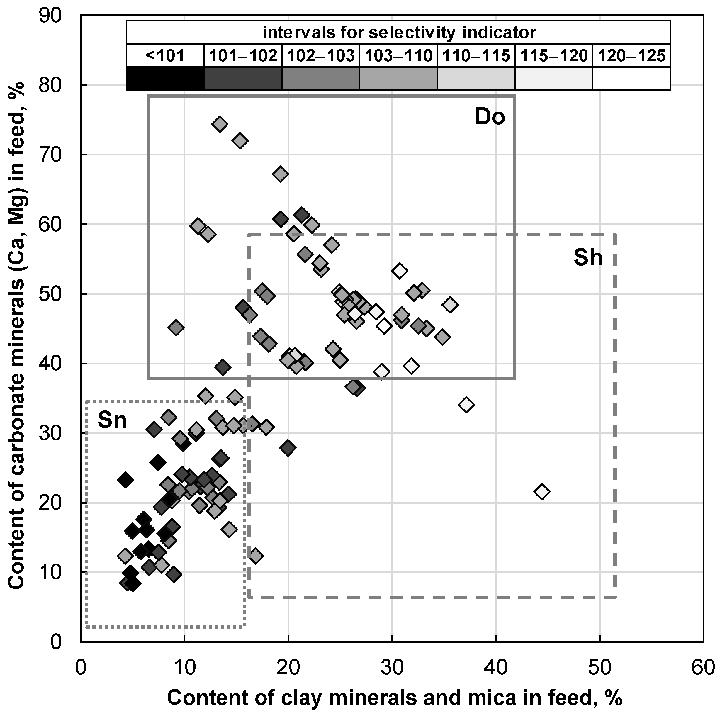
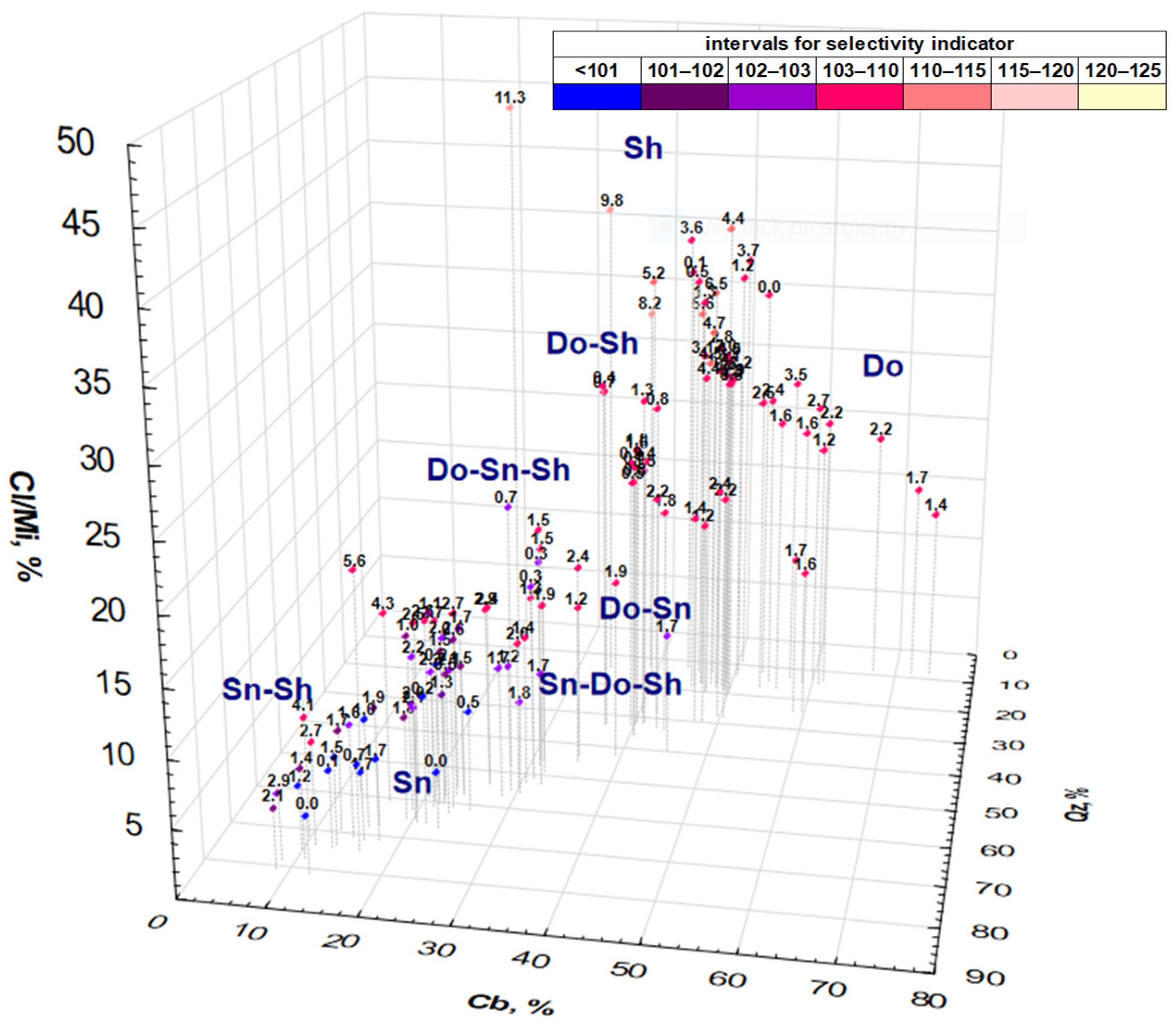
  • The metallurgical effectiveness of the enrichment process of individual lithological compositions depends mainly on two factors: sulfide mineralization, which has a major influence on the quality of the feed and the concentrate (contents of the main metals), and the relationship between the content of carbonate and clay minerals in the feed, which affects enrichment selectivity.
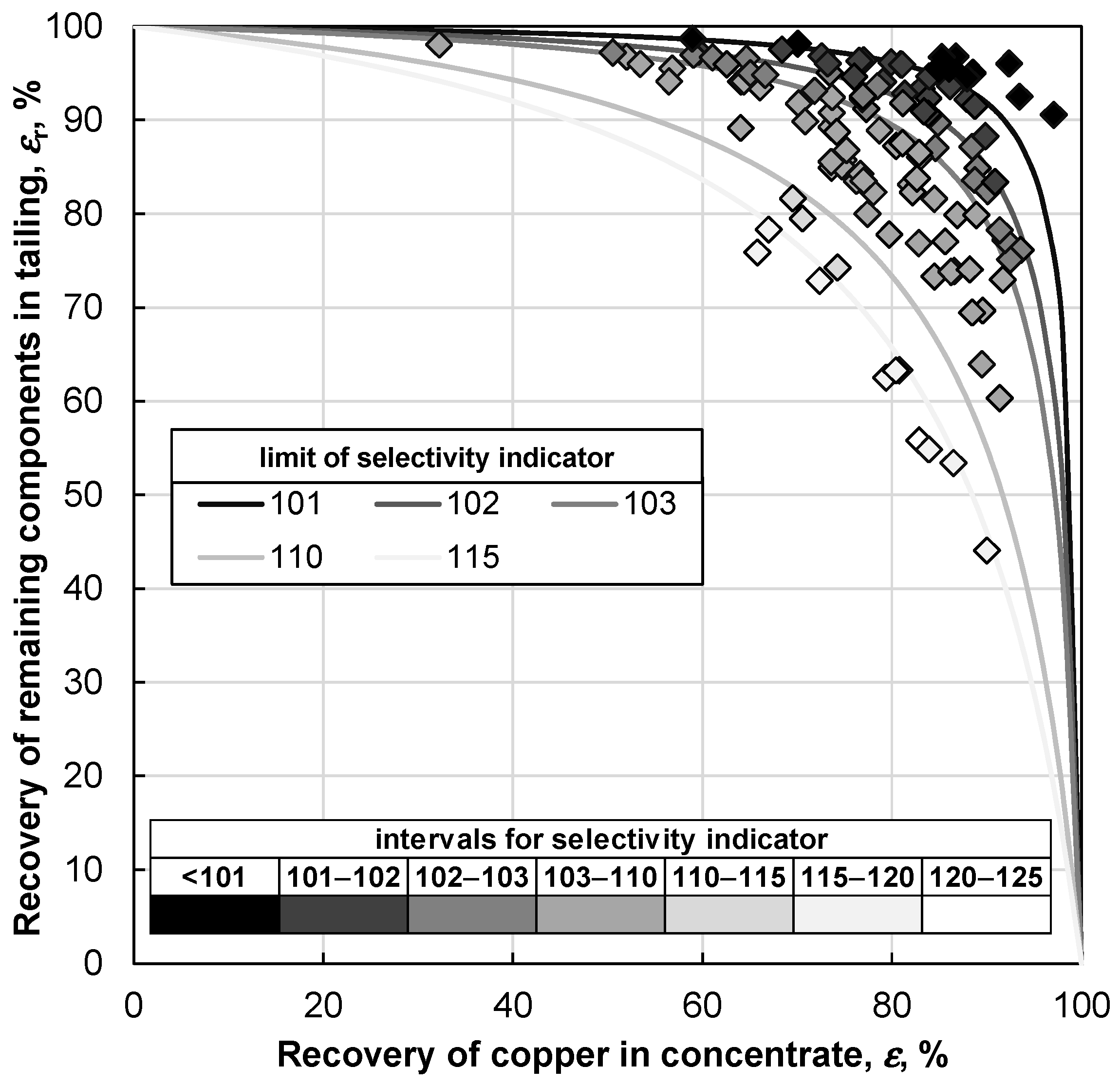
  • Dolomitic–shale mixtures with high contents of clay minerals and low contents of carbonate minerals show the lowest metallurgical enrichment effectiveness (and this being despite the high copper content in the feed). The highest enrichment selectivity was found for sandstone–shale mixtures in which shale represented 10% of the mixture mass; these were mixtures with low contents of carbonate minerals and high contents of quartz,
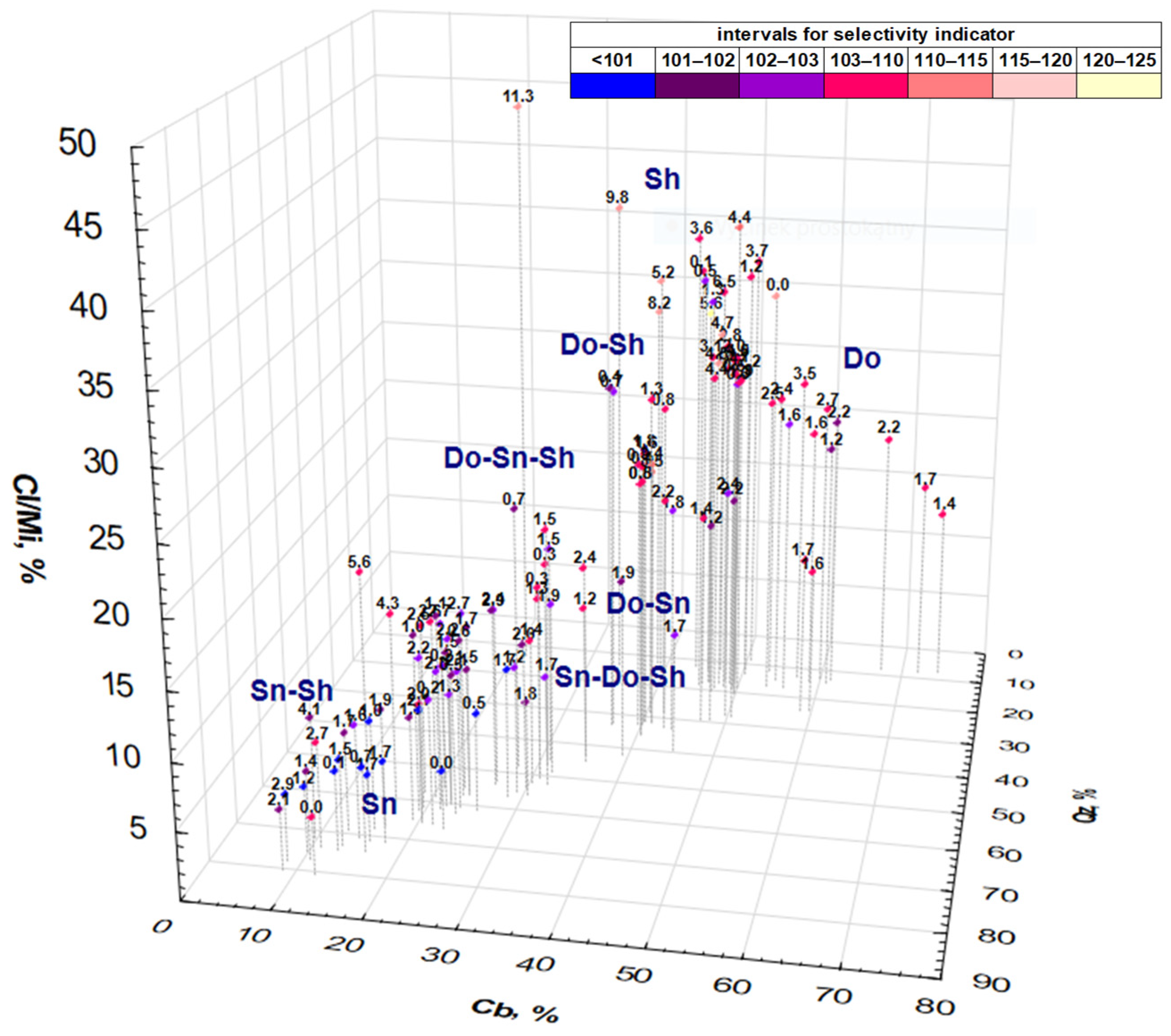
  • In the case of three-component mixtures, higher enrichment effectiveness was observed for the feed mixtures in which quartz was the dominating component (sandstone ore) than for the mixtures in which carbonate minerals dominated (dolomitic ore).
  • The proposed equation performs quick and effective predictions of the copper ore enrichment results from its mineral and chemical composition. It also allows quick and effective control of the performance of the enrichment process, based only on the results of the carbonate and clay minerals and the copper content in the feed of the flotation process. In addition, the derived equation is universal and allows control of the enrichment process depending on the quality parameters of the feed that enters enrichment plants. It also allows this system to be controlled in case of problems during the enrichment process, for example, by changing the lithological composition of the feed entering the process. The use and consideration of this information during enrichment under technological conditions can improve the selectivity of enrichment by effectively monitoring and controlling the composition of the feed entering the enrichment process.
The implementation of geometallurgical modeling in the management of the technological systems operated by KGHM Polska Miedz SA may significantly improve the economic indicators of the production processes. Of course, further considerations are required in terms of the accuracy of the proposed solution by using and testing other statistical modeling methods. Further studies on the enrichment of copper ore with different lithological compositions are needed to expand the database for verifying the derived model, as well as to create new more accurate models. The relationship between the contents of mineral and chemical components in the feed entering the processing plant should be considered at the stage of controlling the ore extraction operations.
The next step in this study, conducted by the authors in cooperation with KGHM Polska Miedz SA, is building a full model of the deposit, consisting of the verification of the model to be applied in at industry scale in order to directly transition the laboratory results to industrial application.

Author Contributions

Conceptualization M.D. and A.B.; methodology, M.D. and A.B.; software, M.D. and A.B.; validation, M.D. and A.B.; formal analysis, M.D. and A.B.; resources, M.D. and A.B.; writing—original draft preparation, M.D. and A.B.; writing—review and editing, M.D. and A.B.; visualization, M.D.; supervision, M.D. All authors have read and agreed to the published version of the manuscript.

Funding

This research presented in this paper was partially financially supported by the project entitled “Ongoing monitoring of the quality of extracted ore in terms of its geometallurgical properties based on a 3D deposit model”, which was carried out by the Wroclaw University of Science and Technology (WUST) as a leader. The source of funding was KGHM Polska Miedz SA. This research was also funded by the Polish Ministry of Education and Science, subsidy 2024, for the Department of Mining (WUST), grant number 8211104160.

Data Availability Statement

Data are contained within the article.

Acknowledgments

We would like to express our appreciation to Andrzej Luszczkiewicz for discussion, patient guidance, and useful comments on this research work.

Conflicts of Interest

The authors declare no conflicts of interest. The funders had no role in the design of this study; in the collection, analyses, or interpretation of the data; in the writing of this manuscript; or in the decision to publish the results.

References

  1. Dobby, G.; Bennett, C.; Bulled, D.; Kosick, G. Geometallurgical modeling-The new approach to plant design and production forecasting/planning, and Mine/Mill Optimization. In Proceedings of the 36th Annual Meeting of the Canadian Mineral Processors, Ottawa, ON, Canada, 20–22 January 2004; Paper 15. [Google Scholar]
  2. Dunham, S.; Vann, J. Geometallurgy, geostatistics and project value–does your block model tell you what you need to know. In Proceedings of the Project Evaluation Conference, Melbourne, Australia, 19–20 June 2007; pp. 1–9. [Google Scholar]
  3. Jackson, J.; Mcfarlane, A.J.; Hoal, K.O. Geometallurgy—Back to the future: Scoping and communicating geomet. In Proceedings of the First AusIMM International Geometallurgy Conference, Brisbane, Australia, 5–7 September 2011; pp. 125–131. [Google Scholar]
  4. Parian, M.; Lamberg, P.; Möckel, R.; Rosenkranz, J. Analysis of mineral grades for geometallurgy: Combined element-to-mineral conversion and quantitative X-ray diffraction. Miner. Eng. 2015, 82, 25–35. [Google Scholar] [CrossRef]
  5. Dominy, S.C.; O’Connor, L.; Parbhakar-Fox, A.; Glass, H.J.; Purevgerel, S. Geometallurgy—A route to more resilient mine operations. Minerals 2018, 8, 560. [Google Scholar] [CrossRef]
  6. Mu, Y.; Salas, J.C. Data-Driven Synthesis of a Geometallurgical Model for a Copper Deposit. Processes 2023, 11, 1775. [Google Scholar] [CrossRef]
  7. Celik, I.B.; Can, N.M.; Sherazadishvili, J.O.H.N. Influence of process mineralogy on improving metallurgical performance of a flotation plant. Miner. Process. Extr. Metall. Rev. 2010, 32, 30–46. [Google Scholar] [CrossRef]
  8. Li, W.; Li, Y.; Yang, X.; Wang, Z.; Chen, W. Process mineralogy assisted iso-floatability of copper-zinc-lead minerals from iron tailings at marcona iron ore mine. Miner. Process. Extr. Metall. Rev. 2023, 46, 129–142. [Google Scholar] [CrossRef]
  9. Michaux, S.; O’Connor, L. How to Set Up and Develop a Geometallurgical Program; GTK Open Work File Report 72/2019; Economic Minerals Unit, Geological Survey of Finland: Espoo, Finland, 2020; pp. 1–245. [Google Scholar]
  10. Bulled, D.; McInnes, C. Flotation plant design and production planning through geometallurgical modelling. SGS Miner. Serv. Tech. Bull. Publ. Ser. 2005, 3, 809–814. [Google Scholar]
  11. Lamberg, P. Particles–the bridge between geology and metallurgy. In Proceedings of the Mineral Engineering, Luleå, Sweden, 8–9 February 2011; pp. 8–9. [Google Scholar]
  12. Lishchuk, V.; Koch, P.H.; Ghorbani, Y.; Butcher, A.R. Towards integrated geometallurgical approach: Critical review of current practices and future trends. Miner. Eng. 2020, 145, 106072. [Google Scholar] [CrossRef]
  13. Lund, C.; Lamberg, P.; Lindberg, T. Development of a geometallurgical framework to quantify mineral textures for process prediction. Miner. Eng. 2015, 82, 61–77. [Google Scholar] [CrossRef]
  14. Hoal, K.O. Getting the Geo into Geomet. SEG Discov. 2008, 73, 1–15. [Google Scholar] [CrossRef]
  15. Mwanga, A.; Rosenkranz, J.; Lamberg, P. Testing of ore comminution behavior in the geometallurgical context—A review. Minerals 2015, 5, 276–297. [Google Scholar] [CrossRef]
  16. Babel, B.; Penz, M.; Schach, E.; Boehme, S.; Rudolph, M. Reprocessing of a Southern Chilean Zn Tailing by Flotation—A Case Study. Minerals 2018, 8, 295. [Google Scholar] [CrossRef]
  17. Büttner, P.; Osbahr, I.; Zimmermann, R.; Leißner, T.; Satge, L.; Gutzmer, J. Recovery potential of flotation tailings assessed by spatial modelling of automated mineralogy data. Miner. Eng. 2018, 116, 143–151. [Google Scholar] [CrossRef]
  18. Bowell, R.; Brough, C.; Barnes, A.; Vardanyan, A. Geometallurgy of Trace Elements in the Hrazdan Iron Deposit. Minerals 2021, 11, 1085. [Google Scholar] [CrossRef]
  19. Yenial-Arslan, U.; Jefferson, M.; Curtis-Morar, C.; Forbes, E. Pathway to Prediction of Pyrite Floatability from Copper Ore Geological Domain Data. Minerals 2023, 13, 801. [Google Scholar] [CrossRef]
  20. Navarra, A.; Grammatikopoulos, T.; Waters, K. Incorporation of geometallurgical modelling into long-term production planning. Miner. Eng. 2018, 120, 118–126. [Google Scholar] [CrossRef]
  21. Wackernagel, H. Multivariate Geostatistics An Introduction with Applications; Springer: Berlin/Heidelberg, Germany, 1995. [Google Scholar] [CrossRef]
  22. Garrido, M.; Ortiz, J.M.; Sepúlveda, E.; Farfán, L.; Townley, B. An overview of good practices in the use of geometallurgy to support mining reserves in copper sulfides deposits. In Proceedings of the 15th International Conference on Mineral Processing and the 6th International Seminar on Geometallurgy, Santiago, Chile, 20–22 November 2019. [Google Scholar]
  23. Johnson, R.A.; Wichern, D.W. Applied Multivariate Statistical Analysis; Prentice Hall: New York, NY, USA, 2007. [Google Scholar]
  24. Napier-Munn, T.J. Statistical methods to compare batch flotation grade-recovery curves and rate constants. Miner. Eng. 2012, 34, 70–77. [Google Scholar] [CrossRef]
  25. Tumidajski, T. Aktualne tendencje w opisie i modelowaniu matematycznym procesow przerobki materialow uziarnionych [Actual tendencies in description and mathematical modeling of mineral processing]. Gospod. Surowcami Miner.—Miner. Resour. Manag. 2010, 26, 111–121. (In Polish) [Google Scholar]
  26. Tumidajski, T.; Saramak, D.; Foszcz, D.; Niedoba, T. Methods of modeling and optimization of work effects for chosen mineral processing systems. Acta Montan. Slovaca 2005, 1, 115–120. [Google Scholar]
  27. Konieczny, A.; Pawlos, W.; Jach, M.; Pepkowski, R.; Krzeminska, M.; Kaleta, R. Zastosowanie systemu wizualizacji do sterowania parametrami pracy maszyn flotacyjnych w KGHM Polska Miedz S.A. Oddzial Zaklady Wzbogacania Rud [Application of visualisation system for controlling operating parameters of flotation machines in KGHM Polska Miedz S.A. Division of concentrators]. Gor. i Geologia 2011, 6, 61–71. (In Polish) [Google Scholar]
  28. Borg, G.; Piestrzynski, A.; Bachmann, G.; Püttmann, W.; Walther, S.; Fiedler, M. An Overview of the European Kupferschiefer Deposits. Soc. Econ. Geol. Inc. Spec. Publ. 2012, 16, 455–486. [Google Scholar] [CrossRef]
  29. Rydzewski, A.; Sliwinski, W. Litologia skal zlozowych. In Monografia KGHM Polska Miedz S.A.; A. Piestrzynski, A., Ed.; KGHM Cuprum CBR: Wroclaw, Poland, 2007. [Google Scholar]
  30. Oszczepalski, S.; Speczik, S.; Zielinski, K.; Chmielewski, A. The Kupferschiefer Deposits and Prospects in SW Poland: Past, Present and Future. Minerals 2019, 9, 592. [Google Scholar] [CrossRef]
  31. Chmielewski, T. Development of a hydrometallurgical technology for production of metals from KGHM Polska Miedz S.A. concentrates. Physicochem. Probl. Miner. Process. 2015, 51, 335–350. [Google Scholar] [CrossRef]
  32. KGHM Report. Integrated Report of KGHM Polska Miedz S.A. and the KGHM Polska Miedz S.A. Group for 2022. 2022. Available online: https://kghm.com/sites/default/files/2024-01/kghm-integrated-report-2022_7.pdf (accessed on 1 January 2024).
  33. Bakalarz, A.; Duchnowska, M. Analysis of the Possibility of Copper Recovery from Flotation Stratiform Copper Ore Tailings. Miner. Process. Extr. Metall. Rev. 2024, 45, 943–949. [Google Scholar] [CrossRef]
  34. Kijewski, P.; Leszczynski, R. Wegiel organiczny w rudach miedzi—Znaczenie i problemy [Organic carbon in copper ores—Importance and problems]. In The Bulletin of the Mineral and Energy Economy Research Institute of the Polish Academy of Sciences (Zeszyty Naukowe Instytutu Gospodarki Surowcami Mineralnymi i Energia Polskiej Akademii Nauk); Mineral and Energy Economy Research Institute of the Polish Academy of Sciences: Kraków, Poland, 2010; Volume 79, pp. 131–146. (In Polish) [Google Scholar]
  35. Luszczkiewicz, A.; Duchnowska, M.; Drzymala, J.; Konopacka, Z.; Henc, T.; Laskowski, J.; Karwowski, P. Okreslenie Granicznej Wzbogacalnosci Urobku Przerabianego w O/ZWR Rejon Lubin [Determination of the Limiting Enrichment of Ore Processed in the Lubin Concentrator Plant (KGHM)]; Report Nr I-11/2012/S-28; Instytut Gornictwa Politechniki Wroclawskiej: Wroclaw, Poland, 2012. unpublished data (In Polish) [Google Scholar]
  36. Kaczmarek, W.; Twardowski, M.; Wasilewska-Blaszczyk, M. Praktyczne aspekty modelowania litologicznych typow rud w zlozach Cu-Ag LGOM (Legnicko-Glogowskiego Okregu Miedziowego) [Practical aspects of lithological types modelling in Cu-Ag ore LGOM deposit (Legnica-Glogow Copper District)]. Biul. Panstw. Inst. Geol. 2017, 468, 209–226. (In Polish) [Google Scholar] [CrossRef]
  37. Luszczkiewicz, A.; Wieniewski, A. Kierunki rozwoju technologii wzbogacania rud w krajowym przemysle miedziowym [Directions in development of ore processing technology in Polish copper industry]. Gor. i Geoinzynieria 2006, 30, 181–196. (In Polish) [Google Scholar]
  38. Konieczny, A.; Kasinska-Pilut, E.; Pilut, R. Problemy technologiczne i techniczne procesu przerobki mechanicznej rud miedzi w swietle dzialalnosci i roli Oddzialu Zaklady Wzbogacania Rud KGHM Polska Miedz S.A. [Technological and technical problems in mineral processing of Polish copper ores at division of concentrators KGHM Polska Miedz SA]. Cuprum Czas. Nauk.-Tech. Gor. Rud 2009, 1–2, 31–46. (In Polish) [Google Scholar]
  39. Pawlos, W.; Poznar, E.; Krzeminska, M. The effect of lithological diversity of feed on process efficiency indexes in KGHM Polska Miedz S.A. Concentrator Plants. Biul. Panstw. Inst. Geol. 2017, 469, 67–74. [Google Scholar] [CrossRef]
  40. Sawlowicz, Z. Organic Matter and its Significance for the Genesis of the Copper-Bearing Shales (Kupferschiefer) from the Fore-Sudetic Monocline (Poland). In Bitumens in Ore Deposits. Special Publication of the Society for Geology Applied to Mineral Deposits, 9; Parnell, J., Kucha, H., Landais, P., Eds.; Springer: Berlin/Heidelberg, Germany, 1993. [Google Scholar] [CrossRef]
  41. Oszczepalski, S. Origin of the Kupferschiefer polymetallic mineralization in Poland. Miner. Depos. 1999, 34, 599–613. [Google Scholar] [CrossRef]
  42. Hitzman, M.W.; Selley, D.; Bull, S. Formation of sedimentary rock-hosted stratiform copper deposits through Earth history. Econ. Geol. 2010, 105, 627–639. [Google Scholar] [CrossRef]
  43. Tomaszewski, J. Problems of a rational utilization of copper-polymetallic ores from the Foresudetic Monocline deposits. Physicochem. Probl. Miner. Process. 1985, 17, 131–141. Available online: https://www.journalssystem.com/ppmp/pdf-80391-35434?filename=The%20problems%20of%20the.pdf (accessed on 1 January 2024). (In Polish).
  44. Konstantynowicz-Zielinska, J. Petrografia i geneza lupkow miedzionosnych monokliny przedsudeckiej. Rudy Met. Niezelaz. 1990, 35, 128–137. (In Polish) [Google Scholar]
  45. Kucha, H. Mineralogia kruszcowa i geochemia ciala rudnego zloza Lubin-Sieroszowice. Biul. Panstw. Inst. Geol. 2007, 423, 77–94. (In Polish) [Google Scholar]
  46. Skorupska, B.; Wieniewski, A.; Kubacz, N. Mozliwosci produkcji koncentratow miedziowych o zroznicowanej zawartosci skladnikow organicznych [Possibility of copper concentrates production of different organic elements content]. Gor. i Geologia 2011, 6, 201–216. (In Polish) [Google Scholar]
  47. Wasilewska-Blaszczyk, M.; Twardowski, M.; Mucha, J.; Kaczmarek, W. Model litologiczny 3D przy zastosowaniu technik interpolacyjnych i symulacji geostatystycznej (na przykladzie zloza Cu-Ag Legnicko-Glogowskiego Okregu Miedziowego) [3D lithological model using by interpolation and simulation methods on an example of the Cu-Ag deposit, Legnica-Głogow Copper District]. Biul. Panstw. Inst. Geol. 2017, 468, 237–246. (In Polish) [Google Scholar] [CrossRef]
  48. Twardowski, M.; Kaczmarek, W.; Rozek, R. Trzeci wymiar geologii zloza rud miedzi [The third dimension of the geology of copper ore deposit]. Prz. Geol. 2020, 68, 886–893. (In Polish) [Google Scholar]
  49. Bakalarz, A.; Duchnowska, M.; Luszczkiewicz, A. Ongoing monitoring of the quality of extracted ore in terms of its geometallurgical properties based on a 3D deposit model. Stage 2. Raporty Wydzialu Geoinzynierii, Gornictwa i Geologii Politechniki Wroclawskiej. Report no. 6. 2021; unpublished data. (In Polish) [Google Scholar]
  50. Kubik, R. Creation and development of QEMSCAN®®® analysis procedure based on Polish copper ores investigation. Int. Multidiscip. Sci. GeoConference SGEM Surv. Geol. Min. Ecol. Manag. 2018, 18, 59–66. [Google Scholar]
  51. Kijewski, P.; Lis., J. Warunki geologiczno–inzynierskie w obszarze Zloza [Geological and engineering conditions in the Deposit area]. In Monografia KGHM Polska Miedz S.A.; KGHM Cuprum Sp. z o.o. CBR: Lubin, Poland, 1996; pp. 164–168. (In Polish) [Google Scholar]
  52. Drzymala, J.; Ahmed, H.A.M. Mathematical equations for approximation of separation results using the Fuerstenau upgrading curves. Int. J. Miner. Process. 2005, 76, 55–65. [Google Scholar] [CrossRef]
  53. Duchnowska, M.; Drzymala, J. Self-similarity of upgrading parameters used for evaluation of separation results. Int. J. Miner. Process. 2012, 106, 50–57. [Google Scholar] [CrossRef]
  54. Foszcz, D.; Duchnowska, M.; Niedoba, T.; Tumidajski, T. Accuracy of separation parameters resulting from errors of chemical analysis, experimental results and data approximation. Physicochem. Probl. Miner. Process. 2016, 52, 98–111. [Google Scholar]
  55. Duchnowska, M.; Drzymala, J. Transformation of equation y = a(100 − x)/(a − x) for approximation of separation results plotted as Fuerstenau’s upgrading curve for application in other upgrading curves. Physicochem. Probl. Miner. Process. 2011, 47, 123–130. [Google Scholar]
  56. Hair, J.F.; Black, W.C.; Babin, B.J.; Anderson, R.E.; Tatham, R. Multivariate Data Analysis, 6th ed.; Prentice Hall: Upper Sadle River, NJ, USA, 2006. [Google Scholar]
Figure 1. Stages of geometallurgical modeling (based on [12,13]).
Minerals 15 00432 g001
Figure 3. The enrichment results for lithological ore mixtures shown as a recovery–recovery enrichment curve (the Fuerstenau curve).
Minerals 15 00432 g003
Figure 4. Influence of clay and carbonate minerals on the enrichment selectivity of copper ore; the indicated areas overlap with the composition of pure lithology types: Sn—sandstone, Do—dolomite, and Sh—shale.
Minerals 15 00432 g004
Figure 5. Influence of main rock-forming minerals in copper ore on enrichment selectivity of its lithology mixtures.
Minerals 15 00432 g005
Figure 6. Comparison of the real selectivity indicator value with the value of the indicator calculated from the regression equation.
Minerals 15 00432 g006
Figure 7. Influence of mineral composition on enrichment selectivity for values of selectivity indicator calculated with correlation equation.
Minerals 15 00432 g007
Table 1. The KGHM Polska Miedz SA production for 2022 (calculations based on the KGHM report (2022) [32]).
Mass of mined ore, tons30,500,000
Average Cu content in ore, %1.45
Average Cu content in concentrate, %22.36
Mass of Cu in ore, tons442,700
Concentrate mass, tons1,755,000
Mass of Cu in concentrate, tons392,500
Total final Cu recovery, %88.75
Flotation tailings mass, tons28,717,443.57
Table 2. Cu content and mineral composition of the three examined lithological types of copper ore.
Location of Sample
Collection
Lithology TypeContent, %
CuOre MineralsCct/Dg/DjBnCcpCvTnt/TtrEngPy/MrcGnSpQzCbCl/Mi
LU III/18S1.652.000.920.410.070.250.090.010.250.000.0071.5415.894.96
Sh3.735.602.071.960.240.390.090.010.820.000.008.8750.4832.88
D1.412.480.840.770.310.160.000.000.410.000.008.0674.3713.40
LU-XVII/2S1.691.401.260.020.010.100.000.000.010.000.0071.4617.576.07
Sh6.476.775.920.380.020.430.010.000.020.000.0012.9146.9730.91
D2.172.591.620.290.250.190.000.000.220.000.0013.2961.3221.29
GL-XXVI/1S1.532.510.301.430.180.120.010.000.350.010.1273.4013.326.54
Sh5.569.050.377.720.240.280.000.000.280.030.1413.0345.3629.23
D1.482.720.021.680.630.060.000.000.320.000.0017.8849.2826.49
GL-XXIX/1S1.382.370.460.720.170.200.040.000.520.040.2277.4510.726.60
Sh4.088.890.194.772.480.130.020.000.650.430.2313.8948.8825.28
D0.091.450.000.000.180.000.000.000.960.140.1618.6045.0133.32
SI-XII/1FS2.101.780.510.430.080.500.020.000.220.000.0380.738.474.51
Sh9.8111.348.531.430.031.140.020.000.020.030.1414.2134.0437.15
D1.622.230.640.660.270.300.000.000.350.000.0017.2755.6821.61
SI-XVI/6S0.070.280.000.000.090.010.000.000.170.010.0074.4012.965.78
Sh8.2515.712.277.413.532.280.050.010.150.010.0012.4938.7928.99
D0.541.750.010.260.580.040.000.000.860.000.0019.0249.1525.52
SI-V/5S0.030.050.010.020.010.000.000.000.000.000.0066.7623.264.30
Sh4.394.053.730.050.000.270.000.000.000.000.0010.3548.4135.59
D4.445.084.640.050.000.380.000.000.010.000.0020.1246.9725.40
SI-XVII/2S0.010.020.000.000.000.000.000.000.010.000.0081.0512.304.28
Sh7.169.584.923.600.220.590.080.010.050.090.0213.5650.2624.92
D0.622.120.000.610.460.040.000.000.470.510.0220.7349.8025.19
RU-XXIII/6S1.251.990.201.190.100.150.020.000.320.000.0175.569.874.78
Sh5.228.731.725.100.300.950.010.000.560.010.0815.4839.6031.85
D1.171.870.280.870.250.130.000.000.280.000.0614.3060.7319.27
RU-XI/1S2.942.642.160.010.000.470.000.000.000.000.0078.428.375.01
Sh11.2916.8413.100.860.140.800.000.000.750.760.4413.2221.5644.43
D2.941.420.000.000.010.000.000.000.660.180.5811.7553.2930.73
S, Sh, D—sandstone, shale, dolomite; Cct/Dg/Dj—chalcocite/digenite/djurleite; Bn—bornite; Ccp—chalcopyrite; Cv—covellite, Tnt/Ttr—tennantite/tetrahedrite; Eng—enargite; Py/Mrc—pyrite/marcasite; Gn—galena; Sp—sphalerite; Qz—quartz; Cb—Ca, Mg carbonates; Cl/Mi—clay minerals + micas.
Table 3. Lithology of the test samples.
Sample No.Lithology Content in the Sample, %
DolomiteShaleSandstone
110000
201000
300100
450-50
575-25
625-75
77030-
89010-
9-3070
10-1090
1125570
1270525
Table 5. Summary of linearized nonlinear variable-dependent regression (selectivity indicator) versus independent variables—contents of copper and carbonate and clay minerals in the feed.
Summary of Variable-Dependent Regression
R= 0.777, R2 = 0.604, Corrected R2 = 0.600
F(3.116) = 58.844, p < 0.0000, Standard Estimation Error: 2.897
VariableStandardized Coefficient b*Partial CorrelationSemi-Partial CorrelationToleranceR-SquaredT-ValueProbability Value p
αCb, %0.1630.1890.1210.5500.4502.0670.041
αCl/Mi, %0.2920.2910.1910.4300.5703.2720.001
αCu, %0.5250.5720.4390.6990.3017.5020.000
Standardized coefficient b*St. err. of b*Unstandardized coefficient bSt. err. of bt-valueprobability value p
Free term 97.4680.715136.3320.000
αCb, %0.1630.0790.0480.0232.0670.041
αCl/Mi, %0.2920.0890.1510.0463.2720.001
αCu, %0.5250.0701.2950.1737.5020.000
Disclaimer/Publisher’s Note: The statements, opinions and data contained in all publications are solely those of the individual author(s) and contributor(s) and not of MDPI and/or the editor(s). MDPI and/or the editor(s) disclaim responsibility for any injury to people or property resulting from any ideas, methods, instructions or products referred to in the content.

