Optimization in Mineral Processing: A Novel Matheuristic for a Variant of the Knapsack Problem

Abstract

This study introduces a novel heuristic approach to optimize mineral processing in metallurgical plants, framed as a variant of the fractional knapsack problem. The optimization framework integrates plant operational modes, blending requirements, and processing constraints to maximize the recoverable value of mineral blocks while adhering to plant capacity and feed limitations. Building on a previously established mixed-integer linear programming formulation, this study develops a heuristic algorithm employing a greedy strategy. This alternative approach significantly reduces computational time while achieving near-optimal solutions, making it suitable for practical implementation. Validation through a case study demonstrates the algorithm’s effectiveness in managing complex constraints and delivering actionable insights for real-world operations. These findings highlight the potential of this methodology to streamline the mineral processing stage of broader mine planning frameworks, complementing the initial optimization of block extraction with faster and more reliable processing calculations.

1. Introduction

Metallurgical plants are central to the mineral value chain, significantly affecting a mine’s operating costs and revenue. A critical example is the comminution process—encompassing crushing and grinding—which liberates valuable minerals for subsequent flotation or leaching. This stage alone often consumes over 30% of a mine’s total energy usage, and as much as 50% of a mine’s electrical energy [1,2,3] and is influenced by ore characteristics such as hardness and liberation size [4]. Consequently, optimizing comminution is crucial for increasing metal recovery while reducing both energy consumption and operational costs [5].

Beyond comminution, additional factors limit the full recovery of valuable metals. For instance, the presence of cyanide-consuming elements—like gold and silver—necessitates higher reagent dosages, driving up operating costs [6]. Inevitably, some fraction of the valuable minerals is lost to tailings [7]. Striking an optimal balance between the final product sold and the material sent to tailings thus becomes essential. This ratio depends on the natural variability of the incoming feed and the extent to which the plant can adapt to these fluctuations, directly impacting both costs and revenues.

Adapting to feed variability often involves reconfiguring the plant to ensure efficient processing. For example, switching from a coarse to a fine grind may require emptying the semi-autogenous grinding (SAG) mill and substituting the existing steel ball load—a procedure that can force the plant to halt or operate below capacity. While such changes can improve recovery, frequent reconfigurations are impractical. Instead, metallurgical plants typically operate within predefined operational modes—sets of parameters (e.g., blending proportions, feed rates, and grinding conditions) specifically suited to certain ore characteristics or production targets [8]. These modes help maintain efficiency and throughput during substantial or prolonged changes in the feed. Additionally, introducing new equipment or sensors may prompt the creation of further operational modes [9,10].

Importantly, these operational decisions also carry significant long-term financial consequences. Choices around reconfiguration, energy consumption, metal recovery, and maintenance can accumulate over the life of a mine, making it essential to capture their effects in strategic mine-planning frameworks. However, despite the importance of operational modes, relatively few models integrate them at a detailed level within long-term mine planning. For instance, Ref. [7] extended stochastic mine-planning algorithms to evaluate net present value (NPV) by incorporating alternative operational modes under geological uncertainty. Lamghari’s variable neighborhood descent (VND) approach [10] provided a statistical foundation to compare plant designs and justify expansions. Ref. [11] observed that, while current long-term mine-planning methods often handle geological uncertainty effectively, they frequently lack robust representations of alternate processing modes. They responded by proposing a computational framework that integrates geometallurgical models, enabling the evaluation of multiple operational modes more accurately.

Production control for mineral processing has been addressed by developing a digital twin framework that combines discrete event simulation (DES) with a customized machine learning (ML) model [12]. The work identifies trigger points for switching operational modes, improving short- and long-term outcomes. However, because this framework relies on simulation rather than a formal optimization model, it does not guarantee a mathematically optimal solution. In contrast, Ref. [8] focused on enhancing stochastic mine-planning algorithms to implement mode changes in greater detail, proposing a two-stage optimization model. In the second stage—representing the metallurgical plant—they introduced a Dantzig–Wolfe decomposition [13] with a linear programming formulation, nested within the stochastic mine-planning algorithm. Ref. [14] then built on that work by applying the ultimate pit limit (UPL) to reduce the number of blocks and parallelizing the VND algorithm. Although these improvements lowered execution times to around 41 min for a case with 13,000 blocks, 2 rock types, and 2 operational modes, such a runtime remains impractical for real open-pit mines containing millions of blocks. Because the Dantzig–Wolfe decomposition is iterated thousands of times within the optimization, even modest per-iteration improvements can significantly reduce the overall runtime. Consequently, further improving this computationally intensive step remains a priority.

Against this backdrop, the present study introduces a matheuristic that balances two objectives: maximizing mineral-processing performance and minimizing deviation from the exact optimal solution. By matheuristics, we refer to heuristic algorithms that integrate metaheuristic and mathematical programming techniques [15]. The proposed approach combines a greedy algorithm with a continuous knapsack subproblem to address efficiently the unique challenges of multi-mode mineral processing, where variations in ore grade and textural characteristics demand adaptive strategies. While the underlying computational framework is essential, our method is grounded in metallurgical principles captured by the operational modes, ensuring that decisions related to ore blending, comminution, and flotation process are informed by the geological and mineralogical properties of the deposit.

This paper begins by reviewing the knapsack problem and its main variants, then discusses how the unique constraints of multi-mode mineral processing depart from standard formulations. Next, we describe the metaheuristic aspects of our approach, underscoring the elements essential for flexible mode selection. We then illustrate the potential of this method through a detailed case study, showcasing its efficacy in maintaining near-optimal solutions within reduced computational times. Finally, we draw conclusions regarding the broader implications of incorporating multiple operational modes into strategic mine planning and suggest possible avenues for future research.

2. Knapsack Problem

The knapsack problem is a well-known combinatorial optimization model that seeks to maximize value while respecting a capacity constraint [16]. Two common variants are as follows:

• 0–1 Knapsack: Each item i $\in$ I can be selected entirely (x_i = 1) or not at all (x_i = 0). Mathematically, we have the following:

$$\max \sum _{i\in I}{v}_i{x}_i$$

(1)

s.t.

$$\sum _{i\in I}{w}_i{x}_i\le K,$$

(2)

$$x_i\in \left\{\mathrm{0,1}\right\},\hspace{1em}\hspace{1em}\forall i\in I,$$

(3)

where v_i is the value of item i, w_i is its weight, and K is the knapsack capacity.

• Fractional knapsack: Items can be partially selected, allowing x_i $\in$ [0, 1]. Its formulation replaces the binary constraints (3) with the following:

$$0\le x_i\le 1,\hspace{1em}\hspace{1em}\forall i\in I,$$

(4)

This enables a fraction of each item i to be included. In the standard fractional knapsack, a simple greedy algorithm that sorts items by their value-to-weight ratio solves the problem optimally in $\mathcal{O}\left(n\log n\right)$ time.

2.1. From Knapsack to Mineral Processing

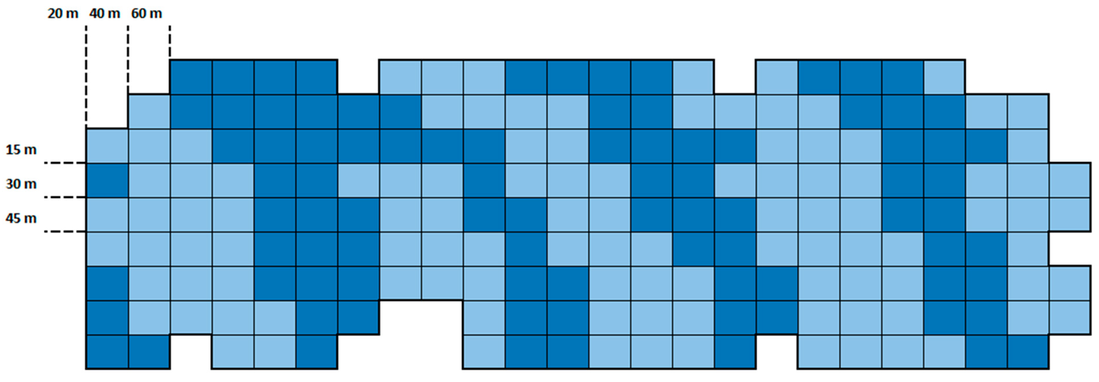
Mineral processing can be conceptually framed as a fractional knapsack problem, especially when an orebody is divided into discrete blocks that can be partially processed. If we draw an analogy, we have the following:

• Items $\leftrightarrow$ Blocks of ore b $\in \mathcal{B}$, each with a specific mas, m_b.
• Value v_i $\leftrightarrow$ Potential revenue v_b from extracting minerals in block b.
• Weight w_i $\leftrightarrow$ Mass m_b, which contributes to a plant’s capacity usage.
• Capacity K $\leftrightarrow$ A limit on how much the plant can process over a given scheduling period.

Therefore, in the simplest case, a metallurgical plant has a fixed capacity K, and each block can be processed either fully or partially, depending on whether it is beneficial to do so. However, real-world mineral-processing scenarios seldom adhere strictly to the basic 0–1 knapsack or fractional assumptions. In practice, operational modes enter the picture. Each operational mode may be viewed as a specific plant configuration or setting, designed to process different blends of the varying rock types, at varying rates. Consequently, multiple constraints arise as follows:

• Multiple rock types: Blocks can belong to distinct rock types, each with unique metallurgical properties.
• Blending requirements: Certain modes may demand specific ratios of rock types to ensure stable metallurgical performance.
• Partial processing across modes: A single block may be partially processed under one mode and partially under another, if this yields higher overall returns and meets blending constraints.
• Time-based capacity: Instead of a simple tonnage limit, the capacity may be measured in hours of plant operation, which must be allocated efficiently among modes and blocks.

2.2. Mathematical Formulation

The mathematical formulation that incorporates the aforementioned aspects is a mixed-integer linear program (MILP) presented in [8].

Table 1. Summary of notation.

Sets
$\mathcal{P}$	Set of rock types.
${\mathcal{B}}_p$	$\mathrm{Set} \mathrm{of} \mathrm{blocks} \mathrm{of} \mathrm{rock} \mathrm{type} p\in \mathcal{P}$.
$\mathcal{B}$	$\mathrm{Set} \mathrm{of} \mathrm{all} \mathrm{blocks}, \mathcal{B}=\bigcup _{p\in \mathcal{P}}{\mathcal{B}}_p$.
$\mathcal{O}$	Set of operational modes.
Parameters
mb	$\mathrm{Mass} \mathrm{of} \mathrm{the} \mathrm{block} b\in \mathcal{B}$.
vbo	$\mathrm{Total} \mathrm{monetary} \mathrm{value} \mathrm{of} \mathrm{block} b\in \mathcal{B}$ $\mathrm{processed} \mathrm{in} \mathrm{mode} o\in \mathcal{O}$.
ro	Tonnage processing rate (ton/h) under mode o.
q	Total available processing time (hours) of the plant.
wop	Required fraction of rock type p in the plant feed under mode o.
Variables
xbo	Mass of block b processed under mode o.

summarizes the notation used throughout.

The objective function and constraints are as follows:

$$\max \sum _{b\in \mathcal{B}}\sum _{o\in \mathcal{O}}\left({\displaystyle \frac{v_{bo}}{m_b}}\right)x_{bo}$$

(5)

s.t.

$$\sum _{b\in \mathcal{B}}\sum _{o\in \mathcal{O}}{\displaystyle \frac{1}{r_o}}{x}_{bo}\le q,$$

(6)

$$\sum _{o\in \mathcal{O}}{x}_{bo}\le m_b,\hspace{1em}\hspace{1em}\forall b\in \mathcal{B},$$

(7)

$$\sum _{b\in {\mathcal{B}}_{p1}}{x}_{bo}={\displaystyle \frac{w_{op1}}{w_{op2}}}\sum _{b\in {\mathcal{B}}_{p2}}{x}_{bo},\hspace{1em}\hspace{1em}\forall o\in \mathcal{O},\forall p_1,p_2\in \mathcal{P},$$

(8)

$$x_{bo}\ge 0,\hspace{1em}\hspace{1em}\forall b\in \mathcal{B},\forall o\in \mathcal{O}.$$

(9)

This formulation maximizes the total recoverable value across all blocks and modes using v_bo/m_b to represent the value per unit mass (Equation (5)). Constraint 6 ensures that the cumulative processing time does not exceed the available hours q. Since (1/r_o) x_bo denotes the time required to process mass x_bo of block b under mode o, the sum of these terms must be less than or equal to q. Constraint 7 limits the total processed mass of each block b to at most m_b. Constraint 8 enforces the blending ratios for rock types within each mode o. Because w_op1 and w_op2 represent the fractional requirements for rock types p₁ and p₂, respectively, their processed masses must reflect the specified ratio. Finally, Constraint 9 ensures the non-negativity of the decision variables.

As mentioned previously, this formulation was implemented in [8] and further refined in [14]. However, the runtime reaches almost 41 min for 13,000 blocks, 2 operational modes, and 2 rock types. Although the Dantzig–Wolfe implementation in these works is highly efficient, the fact that this part of the code is executed thousands of times means that even a minor improvement in the implementation could significantly reduce the overall execution time, especially when scaling to scenarios involving millions of blocks.

3. Matheuristic

We proposed a matheuristic to solve the MILP formulation efficiently to determine the amount of mass of each block b $\in \mathcal{B}$ to be processed under a specific operational mode, o $\in \mathcal{O}$, which maximizes the recoverable value v_bo of the set of blocks $\mathcal{B}$.

The matheuristic consists of the following two phases: the benefit calculation phase and the fraction assignment phase. The benefit calculation phase computes the potential benefit of processing blocks for each operational mode. Once the operational mode with the highest benefit is selected, the fraction assignment phase determines the percentage of the blocks to be processed.

The main algorithm and its two phases are described in the following subsections. Additionally, Appendix A presents a supplementary numerical example that further illustrates how the algorithm operates.

3.1. Main Algorithm

Algorithm 1 describes the main procedure of the matheuristic. It begins with a set of blocks, $\mathcal{B}$; a set of rock types, $\mathcal{P}$; a set of operational modes, $\mathcal{O}$, of the plant; parameters related to the available time of the plant, q; the mass m_b of each block b $\in \mathcal{B}$; the tonnage processing rate r_o by mode o $\in \mathcal{O}$; the value, v_bo, of each block b $\in \mathcal{B}$ processed by mode o $\in \mathcal{O};$ and the proportion requirement, w_op, for each block of rock type p processed by mode o. Then, the best benefit, σ, is initialized as zero, and lists related to the problem information for each iteration of the algorithm—$L_{op}^v$, $L_{op}^t$, $L_{op}^w$, $L_{op}^{OR}$, $L_{op}^{FA}$, and $L_{op}^{{FA}^{\prime }}$—are initialized.

Algorithm 1 Main Algorithm
1:	Inputs: $\mathcal{B}$, $\mathcal{P}$, $\mathcal{O}$, q, mb, ro, vbo, wop
2:	Output: Processed blocks and their assigned fraction ($L_{op}^{FA}$)
3:
4:	Initialization:
5:	σ $⟵$ 0	◊ best benefit
6:	$L_{op}^v$, $L_{op}^t$, $L_{op}^w$, $L_{op}^{OR}$, $L_{op}^{FA}$, $L_{op}^{{FA}^{\prime }}$
7:
8:	Sort all lists $L_{op}^{OR}$ according to non-increasing order of their OR.
9:	while $\mathcal{B}\ne \mathcal{\varnothing }$, q > 0, σ ≥ 0 do
10:	Call o*, σ $⟵$ BENEFIT_CALCULATION($\mathcal{O}$, $\mathcal{P}$, $L_{op}^w$, $L_{op}^{OR}$)
11:	if σ ≥ 0 then
12:	Call FRACTION_ASSIGNMENT($\mathcal{O},\mathcal{P},L_{op}^w,L_{op}^{OR},L_{op}^{FA},L_{op}^{{FA}^{\prime }},m_b,q,o^{*}$)
13:	end if
14:	end while

$L_{op}^v$, $L_{op}^t$, and $L_{op}^w$ remain unchanged at every iteration of the algorithm and are only updated with a new instance of the problem. $L_{op}^v$ stores the recoverable value of each block classified by rock type. It is initialized with the recoverable value, v_bo, of each block b of rock type p when it is processed by mode o. $L_{op}^t$ stores the processing time information for each block classified by rock type p when a specific operational mode, o, is selected. It is initialized with the quotient between the mass, m_b, of the block and the processing ratio, r_o, for each mode o. $L_{op}^w$ saves the proportion requirement information to ensure the correct mix of rock types for each processing mode. It is initialized with the proportion requirement w_op for each rock type p when it is processed by mode o.

$L_{op}^{OR}$, $L_{op}^{FA},$ and $L_{op}^{{FA}^{\prime }}$ are updated at every iteration of the algorithm and allow us to determine a decision path to process blocks in the best operational mode with the correct tonnage quantity, respectively.

• $L_{op}^{OR}$ stores the order ratios (ORs) of the blocks to determine which are potentially more attractive to process, considering different operational modes. These ratios are calculated using the quotient of the values of $L_{op}^v$ and $L_{op}^t$ for each block b of rock type p when processed by mode o. The list is computed once at the algorithm’s beginning and sorted in a non-increasing order. In every iteration, when a block is completely processed, it is eliminated.
• $L_{op}^{FA}$ stores the feasible fractions assigned (FAs) for each block b of rock type p that is processed under different operational modes, o (x_bo/m_b). At each iteration, the FA value for each block is updated to ensure a feasible mix of rock types for each processing mode. The list is initialized with a fraction assignment of zero for each block.
• $L_{op}^{{FA}^{\prime }}$ stores 1 − $L_{op}^{FA}$ to track the remaining portion of each block b that has not yet been processed. Unlike $L_{op}^{FA}$, this list is initialized with a value of 1.

After initialization, the list of blocks $L_{op}^{OR}$ is sorted in non-increasing order based on their ORs. Then the benefit calculation phase and the fraction assignment phase are called until some of the following stop criteria are met: (i) there are no remaining unprocessed blocks, (ii) the processing capacity is fully occupied, or (iii) the best potential benefit offered by a next iteration is negative.

The algorithm concludes by returning a list of processed blocks of rock type p in mode o, along with their assigned fractions $L_{op}^{FA}$. The total value of ore processing is calculated as the product of each block’s value and its corresponding FA. The following subsections, the benefit calculation phase and the fraction assignment phase, are described in detail.

3.2. Benefit Calculation

Algorithm 2 describes the benefit calculation phase, which computes the best potential benefit of processing blocks considering different operational modes. It begins with a set of operational modes, $\mathcal{O}$, of the plant, a set of rock types, $\mathcal{P}$, the proportion requirement, $L_{op}^w$, and the order ratios, $L_{op}^{OR}$. The function outputs the best operational mode o* and the best benefit σ generated by the block of rock type p processed by the best operational mode o*.

Algorithm 2 Benefit Calculation Function
1:	function BENEFIT_CALCULATION($\mathcal{O}$, $\mathcal{P}$, $L_{op}^w$, $L_{op}^{OR}$)
2:	Initialization:
3:	o* $⟵$ none	◊ best operational mode
4:	σ $⟵$ −∞	◊ best benefit in mode o*
5:	total_benefit[o]  $⟵$$0, o \in \mathcal{O}$
6:
7:	for all o $\in \mathcal{O}$ do
8:	Determine rock type p* with the maximum value wop, p $\in \mathcal{P}$
9:	total_benefit[o] $⟵{\sum }_{p\in \mathcal{P}}{(L}_{op}^{OR}$ × $L_{op}^w/L_{o{p}^{*}}^w)$
10:	if total_benefit[o] > σ then
11:	σ $⟵$ total_benefit[o]
12:	o*  $⟵$o	◊ Update best operational mode
13:	end if
14:	end for
15:
16:	return o*, σ
17:	end function

First, we initialize the best mode as none, the best benefit as −∞, and the total benefit at each mode as 0. Then, for each mode, o $\in \mathcal{O}$, we determine the rock type p^* with the maximum w_op in $L_{op}^w$ to compute the relation factor concerning all the other blocks of rock type p $\in \mathcal{P}$ in order to determine the total benefit in mode o $\in \mathcal{O}$, considering only feasible rock type mixes.

In the final evaluation of all operational modes, we obtain the best operational mode o* and the best benefit σ.

3.3. Fraction Assignment

Once the best operational mode o* with the highest benefit σ is selected, the fraction assignment phase determines the proportion of the rock type block that must be processed in the selected mode. This procedure is described in Algorithm 3.

Algorithm 3 Fraction Assignment Function
1:	function FRACTION_ASSIGNMENT($\mathcal{O}$, $\mathcal{P}$, $L_{op}^w$, $L_{op}^{OR}$, $L_{op}^{FA}$, $L_{op}^{{FA}^{\prime }}$, mb, q, o*)
2:	TP $⟵$ ∞	◊ Total tonnage to be processed
3:	for all p $\in \mathcal{P}$ do
4:	Get block b of rock type p with the highest value in $L_{o^{*}p}^{OR}$
5:	ATp $⟵$ mb × ($L_{op}^{{FA}^{\prime }}$−$L_{o^{*}p}^{FA}$)/$L_{o^{*}p}^w$	◊ Available tonnage to be processed
6:	if TP > ATp then	◊ min(TP, ATp)
7:	pmin $⟵$p
8:	TP $⟵$ATp
9:	end if
10:	end for
11:
12:	for all p $\in \mathcal{P}$ do
13:	TRTp $⟵L_{o^{*}p}^w/L_{o^{*}{p}^{min}}^w$ × TP	◊ Tonnage of each rock type to be processed
14:	$L_{o^{*}p}^{FA}⟵L_{o^{*}p}^{FA}$ + TRTp/mb	◊ Update FA for each block
15:	for all o $\in \mathcal{O}$ \ {o*} do
16:	$L_{op}^{{FA}^{\prime }} ⟵$ 1 − $L_{o^{*}p}^{FA}$	◊ Update FA for the same blocks in other modes
17:	end for
18:	q $⟵$q − TRTp/ ro*	◊ Update available plant capacity
19:	end for
20:	end function

The fraction assignment phase begins with a set of operational modes $\mathcal{O}$ of the plant, a set of rock types, $\mathcal{P}$; the order ratios, $L_{op}^{OR}$; the fraction assignments, $L_{op}^{FA}$; the mass of each block, m_b; the proportion requirement, $L_{op}^w$; the available time of the plant, q; and the best mode, o*. At the end, this procedure updates the fraction assignments, $L_{op}^{FA}$, to be processed for the following iterations.

First, for all rock type p $\in \mathcal{P}$, we determine the available tonnage (AT_p) to be processed in the best mode o*, and we set up the total tonnage to be processed, TP, as the min (TP, AT_p), for all p $\in \mathcal{P}$. Then, we compute the tonnage of each rock type to be processed (TRT_p) in order to determine their respective fraction assignment, updating $L_{o^{*}p}^{FA}$. In this process, we ensure that the required fractions of each rock type p must be processed according to the proportion requirement $L_{op}^w$. Also, we update the fraction assignment for each block in the other operational modes for the following iterations $L_{op}^{{FA}^{\prime }}$. Finally, we update the available plant capacity.

3.4. Advantages of the Matheuristic Approach

The matheuristic approach described in this section is particularly advantageous for complex problems where multiple constraints must be satisfied, such as maintaining specific proportions of rock types in different modes while considering plant capacity limitations. By modularizing the key phases of the algorithm, the approach remains flexible and can be adapted to a wide variety of real-world scenarios. The use of separate functions for benefit calculation, fraction assignment, and termination checking ensures that the algorithm remains computationally efficient, even as the number of rock types and operational modes increases.

4. Sample Calculations

4.1. Case Study

This case study builds upon the same fictional Au-Cu porphyry deposit of the Maricunga region in Chile described in [14], which is closely related to the case presented in [9]. Briefly, this deposit is set within the Maricunga belt—a high-Andean region renowned for its numerous gold, silver, and copper prospects and deposits [14]. The belt is characterized by predominantly porphyry–epithermal systems, along with notable vein and distal contact metasomatic deposits. In addition to its mineral processing potential, the deposit exhibits distinct mineralogical and petrographic features. As detailed in [9], gold-rich porphyry deposits such as this are formed by a combination of magmatic, sedimentary, and hydrothermal processes within volcanic–plutonic arcs, typically emplaced at shallow crustal levels. These deposits not only display significant variations in mineral composition and textural characteristics—which influence both mineralization and processing behavior—but are also associated with a range of lithological variations and structural features that underscore their complex geological evolution. The integration of these mineralogical and petrographic aspects offers a more comprehensive perspective on both the genesis of the deposit and the subsequent challenges and opportunities for optimizing mineral processing.

This study develops a conceptual model with a distinct focus on processing minerals, rather than designing a mine plan, as presented in [14], by assuming that the entire orebody is extracted in a single period. The conceptual model centers on an Au-rich porphyry system, incorporating geological elements such as (1) diorite porphyry hosting mineralized veinlets and (2) silicified intrusive breccias. Figure 1 provides a schematic representation of the geological model. The case considers two operational modes in the metallurgical plant, consistent with the parameters presented in [14], to ensure clarity in the analysis and facilitate understanding of the proposed approach. Further details are provided in

Table 2. Parameters of the case study.

Parameters	Values
Block weight (ton)	15,375
Number of blocks	13,392
Block dimension (m)	20 × 20 × 15
Block density (ton/m3)	2.56
Metal price Au (USD/oz)	1190
Processing availability (h/period)	Infinite
Rock types	Diorite porphyry
	Silicified intrusive breccia
Operational Mode A
Processing rate (ton/h)	250
Processing cost (USD/ton)	21.4
Recovery Au (%)	83
Diorite rock (%)	65
Silicified rock (%)	35
Operational Mode B
Processing rate (ton/h)	200
Processing cost (USD/ton)	24.9
Recovery Au (%)	83
Diorite rock (%)	45
Silicified rock (%)	55

.

Unlike the previous study, which analyzed multiple scenarios, this case study evaluates a single scenario, considering that its primary objective is to validate the performance of a matheuristic algorithm for optimizing mineral processing. Consequently, multithreading techniques were not employed. Three dataset sizes—5000, 10,000, and 13,932 blocks—were tested to assess the algorithm’s scalability and robustness. The first two sizes were arbitrarily chosen with increments of 5000 blocks each, while the last size represents the maximum number of available blocks.

The algorithm was implemented in C++ and executed on a laptop computer equipped with a 12th Gen Intel(R) Core(TM) i7-1255U processor running at 1.70 GHz.

4.2. Results

Table 3. Comparison of processed ore for 5000 blocks between the matheuristic and the optimal solution (Gurobi).

Processed Ore (ton)	5000
	Matheuristic	Gurobi	Difference	%
Under Mode A	3,198,164	3,075,000	−123,164	−4.01
Diorite Porphyry	2,078,807	1,998,750	−80,057
Silicified Intrusive Breccia	1,119,357	1,076,250	−43,107
Under Mode B	1,710,714	1,845,000	134,286	7.28
Diorite Porphyry	769,821	830,250	60,429
Silicified Intrusive Breccia	940,893	1,014,750	73,857
Total	4,908,878	4,920,000	11,122	0.23

Notes: The bold line represents the sum of Diorite and Silicified Breccia for mode A.

,

Table 4. Comparison of processed ore for 10,000 blocks between the matheuristic and the optimal solution (Gurobi).

Processed Ore (ton)	10,000
	Matheuristic	Gurobi	Difference	%
Under Mode A	12,305,073	11,838,751	−466,322	−3.94
Diorite porphyry	7,998,297	7,695,188	−303,109
Silicified intrusive breccia	4,306,776	4,143,563	−163,213
Under Mode B	6,279,340	6,918,749	639,409	9.24
Diorite porphyry	2,825,703	3,113,437	287,734
Silicified intrusive breccia	3,453,637	3,805,312	351,675
Total	18,584,413	18,757,500	173,087	0.92

and

Table 5. Comparison of processed ore for 13,392 blocks between the matheuristic and the optimal solution (Gurobi).

Processed Ore (ton)	13,392
	Matheuristic	Gurobi	Difference	%
Under Mode A	12,784,367	11,704,220	−1,080,147	−9.23
Diorite porphyry	8,309,838	7,607,743	−702,095
Silicified intrusive breccia	4,474,529	4,096,477	−378,052
Under Mode B	9,895,174	11,281,404	1,386,230	12.29
Diorite porphyry	4,452,828	5,076,632	623,804
Silicified intrusive breccia	5,442,346	6,204,772	762,426
Total	22,679,541	22,985,624	306,083	1.33

present the results for processing 5000, 10,000, and 13,392 blocks. The results of the matheuristic are compared to the optimum calculated using the Gurobi solver. As shown, the processed ore represents the sum of the tons processed under Mode A and Mode B. Each mode maintains specific rock type proportions, that is, 65% diorite porphyry and 35% silicified intrusive breccia in Mode A, and 45% diorite porphyry and 55% silicified intrusive breccia in Mode B.

In all three instances, the matheuristic shows a preference for processing under Mode A. This indicates that the available quantity of diorite rock was sufficient to maintain the required blending ratio and achieve a processing rate of 250 tons/hr. Mode A also incurs a lower processing cost (USD 21.4/ton) compared to Mode B (USD 24.9/ton), which operates at a lower rate of 200 tons/hr due to the presence of silicified rock.

However, the optimal solution obtained using Gurobi involves a slightly greater utilization of Mode B. Despite this difference in feed tonnages, which affects the extracted Au (

Table 6. Comparison of gold (Au) tonnage obtained from ore processing between the matheuristic and the optimal solution.

Blocks	Matheuristic	Optimum	Deviation
5000	911,652	921,144	1.03%
10,000	3,678,217	3,692,604	0.39%
13,392	4,516,792	4,536,629	0.44%

), the total value difference between the matheuristic and the optimum solution is less than 0.1% (

Table 7. Comparison of the total value of ore processing (USD) between the matheuristic and the optimal solution.

Blocks	Matheuristic	Optimum	Deviation
5000	789,402,044	789,849,623	0.06%
10,000	3,213,290,927	3,214,442,766	0.04%
13,392	3,914,260,903	3,944,600,957	0.08%

). This aligns with Appendix A, where, for a different dataset, the deviation is slightly higher but still minimal (0.16%). Furthermore, processing 13,392 blocks takes only 4 ms with the matheuristic, compared to 80 ms with the Gurobi solver implementation (Figure 2).

The minimal deviation from the optimum value (Table 7) and the high computational efficiency (Figure 2) demonstrate the advantages of this matheuristic compared to other implementations or solvers like Gurobi. These features make the matheuristic particularly suitable for embedding in optimization frameworks as those in mine planning, where it can be repeatedly utilized to analyze the cumulative impact of aggregated deviations.

5. Conclusions

This study introduced a novel matheuristic approach to optimize mineral processing in metallurgical plants, formulated as a variant of the fractional knapsack problem. The proposed method integrates plant operational modes, blending constraints, and capacity limitations to maximize the recoverable value of mineral blocks. By leveraging a greedy strategy within a heuristic framework, the algorithm significantly reduces computational time while maintaining near-optimal solutions. Validation through a case study demonstrated its ability to effectively manage complex constraints, reinforcing its practical applicability in real-world mining operations.

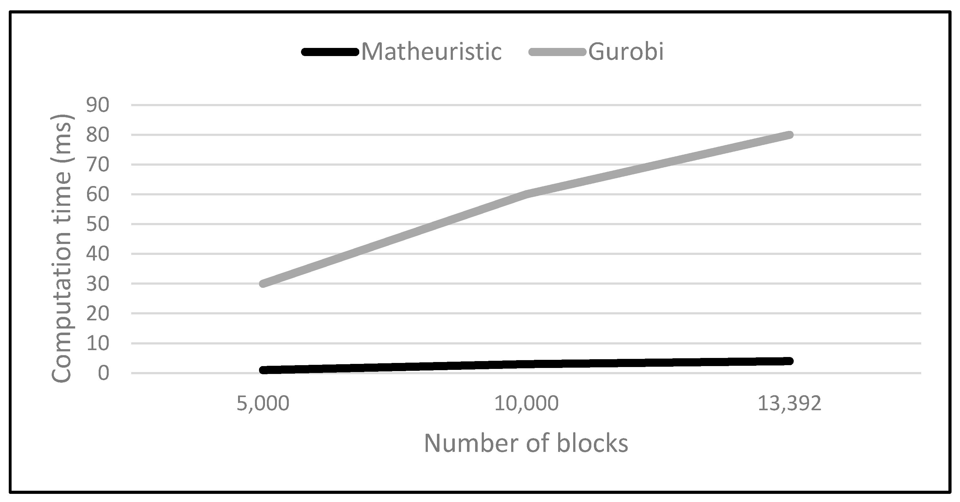
Despite minor deviations from the optimal solution in the case study—less than 0.1% in total value—the proposed algorithm drastically reduces computation time, highlighting its superior efficiency in comparison to exact methods implemented in the Gurobi solver. Additionally, in the case study, the matheuristic successfully maintains blending requirements and operational constraints, ensuring feasible and efficient processing strategies. The preference for operational Mode A over Mode B in the results suggests an inherent flexibility in adapting to different mineralogical compositions and plant configurations, consistent with previous studies that consider multiple processing modes [6,7,8,9,11,12,14].

Given that the current implementation achieves near-optimal results, future research will focus on analyzing whether fine-tuning specific algorithmic components can further enhance performance. In addition, we plan to explore the integration of additional elements—such as accounting for variations in valuable component content across the block and addressing challenges related to geological sampling—to improve the reliability of our forecasting approach. Moreover, while cyanide consumption is currently incorporated indirectly within the processing cost and recovery parameters, future work will investigate modeling the direct costs and usage of reagents like cyanide, further refining the representation of processing economics. On the other hand, this matheuristic is intended to replace the existing Dantzig–Wolfe decomposition-based implementation described by [14], providing a more computationally efficient alternative implementation for the second stage of a formulation relating to a stochastic long-term open-pit mine planning optimization.

Finally, further investigations will explore strategies to ensure that the matheuristic consistently achieves optimal solutions. This includes integrating additional heuristics or hybrid optimization techniques to enhance solution precision while maintaining computational efficiency. The findings of this study pave the way for broader applications of heuristic-based optimization in the mining industry, offering a balance between accuracy and scalability in decision-support frameworks.