3.1. The Data
Two types of datasets are available in this study: (1) the exploration drillhole data and (2) the post-mining survey data. The provenance of these datasets is detailed in previous studies [
1,
10], which describe the methods used for estimating the lateral variability between the bauxite and underlying ferricrete sections, as well as the uncertainty associated with the bauxite ore volume.
The first type of dataset is from 33 vertical drillholes on a regular grid of m at a lateritic bauxite mine site covering an area of approximately 288,000 . The samples, assayed mainly for alumina (Al2O3%) and silica (SiO2%) grades, were collected from each drillhole with a sampling interval of m. These data are used to create the bauxite ore’s thickness intercepts, which are then converted into a two-dimensional point dataset, the variables of which include bauxite floor elevation and bauxite thickness.
The second type of dataset was acquired by surveying the mine floor topography after the mining activity (i.e., extraction of the loose bauxite pisolites by a large front-end loader) was completed at the mine site. The total number of surveying points is 10,934, and the average surveying distance is approximately eight meters. The available drillhole data are used to demonstrate the methodology, while the post-mining survey data are used to compare the results. The sampling locations of both datasets are shown in
Figure 2.
As it can be noticed from
Figure 2a, there appears to be a systematic decrease in the values of the bauxite floor elevations along the north–west to south–east directions, indicating the presence of a large-scale trend in the data. The bauxite thickness values (
Figure 2b), on the other hand, exhibit a stationary behavior throughout the mine site. The survey points (
Figure 2c), which provide a high-resolution representation of the mine floor topography after mining, cover a larger area than the available drillholes. To compare the results, the polygon defining the mine site, excluding the non-surveyed areas, is used to clip the estimated and simulated models (
Figure 2c).
At the time of mining, the determination of the interface between the bauxite ore and underlying ferricrete (or locally known as ironstone) units is based—to a larger extent—on the experience of the front-end loader operator. In other words, there is additional uncertainty associated with the shape of the bauxite/ferricrete contact due to the operator’s skill and experience.
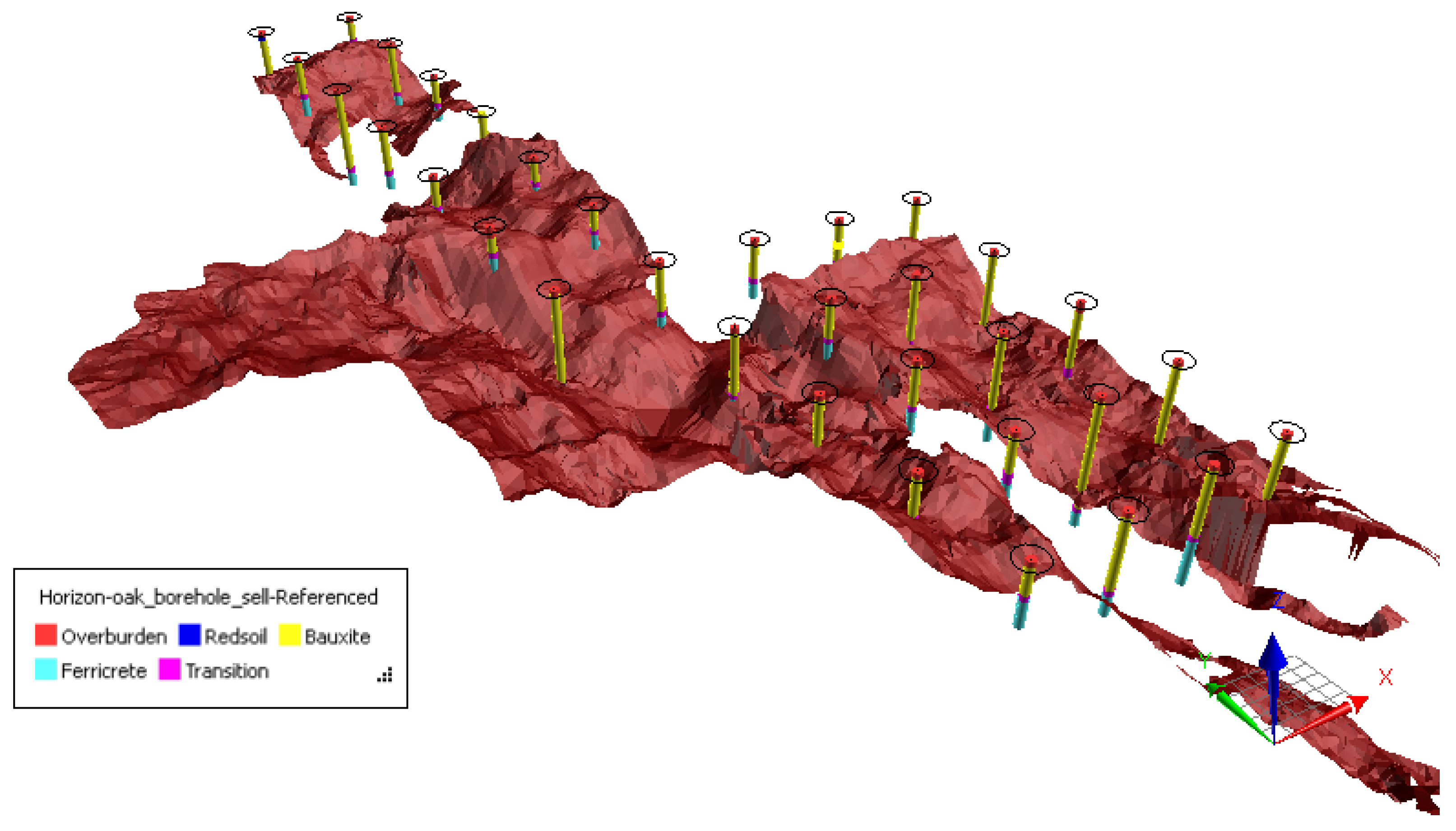
Figure 3 presents the surface of the final mine floor topography along with the drillholes, visualized using the free software Geoscience Analyst (version: 4.5.1) provided by Mira Geoscience.
As shown in
Figure 3, the final mine floor is highly irregular, characterized by random undulations. The deposit is stratified into five lithological units, including overburden, redsoil, bauxite, transition, and ferricrete. It is evident from
Figure 3 that the mine floor elevations determined by the front-end loader operation do not always align with the bauxite floor elevations observed at the drillholes. Therefore, before calculating the bauxite ore volume, the final mine floor elevations must be calibrated based on the bauxite floor elevations observed at the drillholes. The histograms and summary statistics of the variables are shown in
Figure 4.
It is clear from
Figure 2a,b and
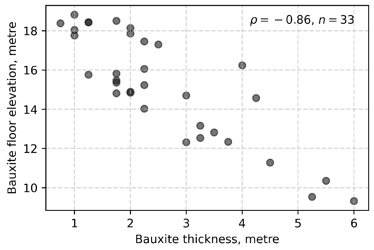
Figure 4a,b that bauxite ore unit tends to become thicker at the topographically low areas and is generally in the form of a thin layer at the topographically high areas, indicating a negative correlation between the values of the bauxite floor elevation and bauxite thickness variables, which is further illustrated in the crossplot presented in
Figure 5.
The scatter plot shown in
Figure 5 reveals a strong negative correlation between bauxite thickness and floor elevation, indicating that thicker bauxite deposits tend to occur at lower elevations.
3.2. Estimation of Bauxite Floor Elevation, Bauxite Thickness, and Mine Floor Topography
To compare the overall bauxite ore volume calculated from the estimated and simulated models against the mined (or actual) bauxite ore volume, the bauxite thickness and the bauxite floor elevations from the drillhole data and mine floor elevations from the post-mining survey data are first interpolated at each grid node
in the mine area. Due to the large-scale trend that exists in the bauxite floor elevations, the local mean cannot be assumed to be constant throughout the entire area; therefore, the KT approach (refer to
Section 2.3) is used to estimate the values of the bauxite floor elevations at all grid nodes.
The trend of order one (i.e., linear trend) is selected to model the trend evident in the bauxite floor elevations. The coefficients of the trend are estimated using the maximum likelihood approach [
32,
33]. The estimated coefficients are as follows:
with
m,
with
m, and
with
m, where SE denotes the standard error. The aforementioned coefficients are, in fact, not used in the KT system, but they are still needed to calculate the residuals. The parameters of the standardized variogram model fitted to the experimental omni-directional variogram of the residuals,
, are given by
The values of the bauxite floor elevations are then estimated at all grid nodes by KT using the variogram model given in Equation (
13).
The bauxite thickness values are estimated at all grid nodes by OK using the standardized spherical variogram model fitted to the experimental omni-directional variogram of the bauxite thickness values:
Considering the abundant post-mining survey data, the mine floor elevations are interpolated at all grid nodes using the inverse distance squared weighting algorithm.
Figure 6 shows the estimation maps of the bauxite floor elevations, bauxite thickness, and the mine floor elevations, which are clipped to the polygon created.
To compare the mined and estimated bauxite ore volumes, the estimates of the bauxite top elevations
are calculated by adding the estimates of the bauxite thickness
to the estimates of the bauxite floor elevation
. The estimates of the mined bauxite thickness
are then calculated by subtracting the estimates of the bauxite top elevations
from the estimates of the mine floor elevations
(
Figure 6c). It is noted that the estimates of the mine floor elevations are calibrated according to the bauxite floor elevations at the drillholes and that any negative values of the mined bauxite thickness variable is set to zero before calculating the in situ bauxite ore volume.
The bauxite resource calculated from the estimates of the bauxite thickness (
Figure 6b) and from the estimates of the mined bauxite thickness are 395,649
and 418,432
, respectively. The uncertainty associated with the estimated bauxite thickness model (
Figure 6b) cannot be evaluated by the kriging error, as the kriging errors are spatially correlated and cannot be used jointly for the entire mine area. For example, kriging error at one location is related to errors at neighboring locations due to spatial dependence in the data; as a result, these errors cannot be used jointly to characterize uncertainty across the entire domain. Geostatistical simulation is therefore used for assessing the uncertainty associated with the bauxite thickness and bauxite floor elevation variables first by assuming that the trend, histograms, and variogram model parameters are known with certainty and then assuming that the trend, histograms, and variogram model parameters are uncertain.
3.3. Simulation of Bauxite Floor Elevation and Bauxite Thickness Without Parameter Uncertainty
In this case, the joint simulation of the bauxite floor elevation and bauxite thickness variables is carried out, assuming that the large-scale trend evident in the bauxite floor elevations, histograms, and variogram model parameters of both variables are known with certainty.
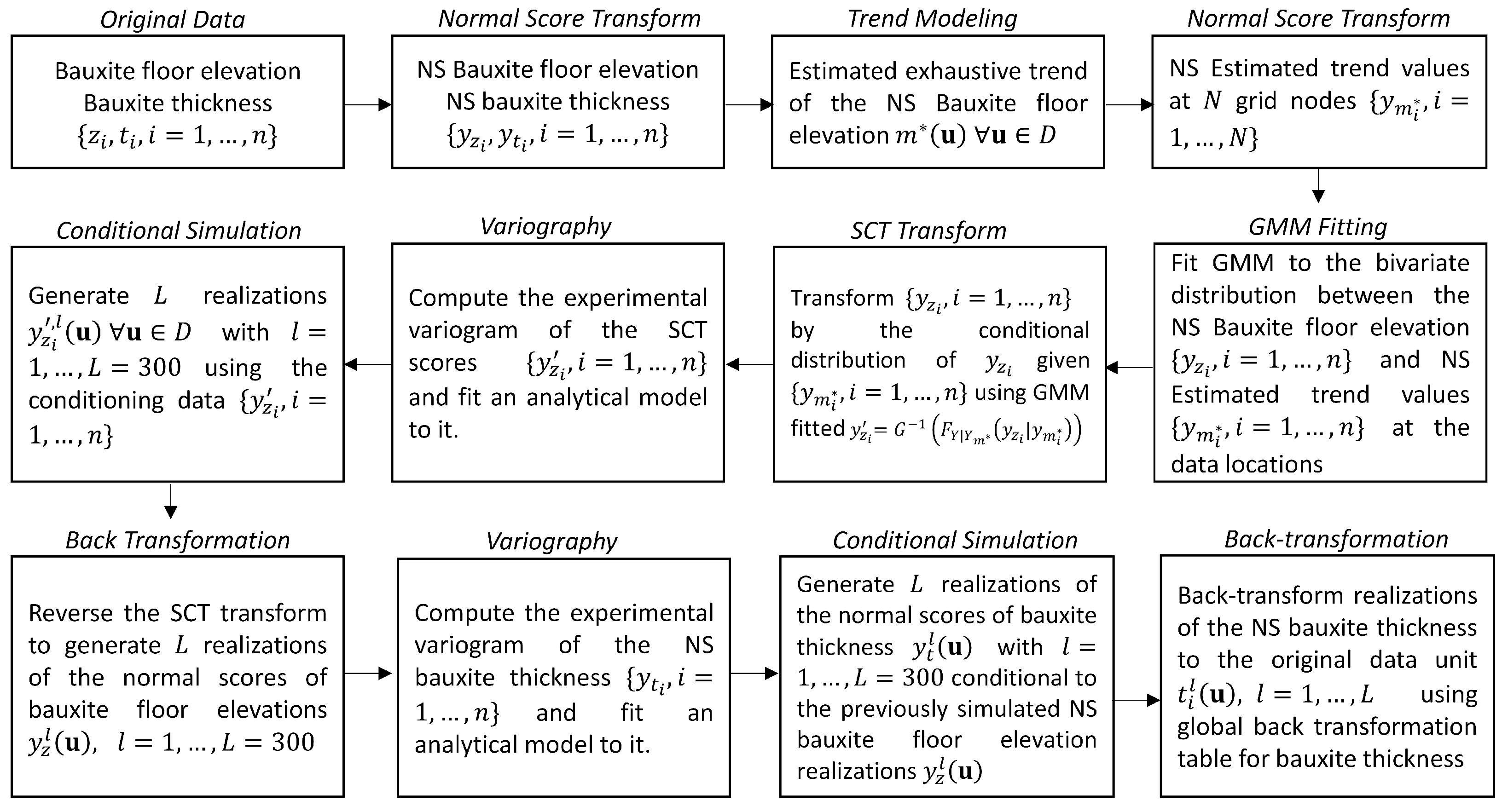
As the drillholes are on a regular grid, declustering is not considered before the transformation of the bauxite floor elevation and bauxite thickness values into the corresponding normal scores. The normal scores of the bauxite floor elevation are used to estimate the trend, indicating only the large-scale variability of the data in the mine area, that is, the trend model should not under- or over-fit the data. The estimated trend values at all grid nodes are then transformed to the normal scores, and the values retained at the data locations are plotted against the normal scores of the bauxite floor elevation, as shown in
Figure 7a.
It can be seen from
Figure 7a that the normal scores of the estimated trend values are highly correlated
with the normal scores of the bauxite floor elevation. The high correlation is explained by the fact that the bauxite floor elevation variable represents position values which are expected to be continuous and closer to the ones estimated by the trend modeling. Because the shape of the crossplot, shown in
Figure 7a, does not exhibit any complexity, a GMM with one component, essentially a single Gaussian distribution, is used to fit the bivariate distribution. A 2D probability density plot representing this bivariate distribution is shown in
Figure 7a. The normal scores of the bauxite floor elevation variable are then transformed by the conditional distribution of the normal scores of the bauxite floor elevation given the normal scores of the estimated trend values. The resulting transformed values (or SCT scores) do not show any correlation with the normal scores of the estimated trend values, as shown in
Figure 7b. It is worth mentioning that in SCT, the order of the variables is important to avoid possible mismatch between the variograms of the simulated realizations and variogram model fitted to the original data. Ref. [
23] suggests that the more continuous variable be selected as the primary variable to minimize the aforementioned mismatch. In this case, the primary variable is represented by the normal scores of the estimated trend values (as this variable is more continuous), and the secondary variable is represented by the normal scores of the bauxite floor elevation variable. The experimental omni-directional variogram of the SCT scores
is then computed and modeled by a standardized spherical (Sph) structure:
The variogram model given in Equation (
15) is used as structural information in the turning bands’ simulation algorithm [
34,
35], which generates unconditionally simulated 300 realizations of the SCT scores on the point support at a grid of
m. The number of turning bands used in the simulation is set to 1000, and the number of simulated points in the domain of the mine area is 25,452. The resulting realizations are conditioned, as a separate step, using simple kriging (SK) [
36].
The back-transformation of the realizations is carried out in the reverse order of the forward transformation, that is, the realizations of the SCT scores are first back-transformed to the realizations of the normal scores of the bauxite floor elevations, and these realizations are then back-transformed to the realizations in the original data unit using the global back-transformation table for the bauxite floor elevations. The randomly selected three realizations of the bauxite floor elevation variable and the E-type model of the bauxite floor elevation variable, calculated by averaging the realizations of the bauxite floor elevation variable in a node-by-node basis, are shown in
Figure 8.
It is clear from
Figure 8 that the large-scale trend evident in the bauxite floor elevations is restored in each realization and that the co-located simulated values honor the original data superimposed on the realizations. It is also clear from
Figure 8 that the trend along the north–west to south–east directions in the original data is restored in the E-type model as well.
The realizations of the bauxite floor elevation variable in the Gaussian unit are then inputted, as exhaustive secondary information, in the turning bands’ simulation algorithm to generate unconditionally simulated 300 realizations of the normal scores of the bauxite thickness variable (refer to
Figure 1 for the implementation steps of the methodology). The structural input required for the simulation is the variogram model fitted to the experimental omni-directional variogram of the normal scores of the bauxite thickness:
The conditioning of the realizations is achieved by the simple intrinsic co-located cokriging (SICCK) approach [
37], where the values of the previously simulated normal scores of the bauxite floor elevation are retained both at the bauxite thickness data locations and at the grid node to be simulated in each local neighborhood. Considering a Markov assumption of conditional independence, i.e., Markov model 1 [
29], the implementation requirements of the SICCK approach are the variogram model given in Equation (
16) and the correlation coefficient
, indicating the strength of the linear relationship between the co-located normal scores of the bauxite thickness and normal scores of the bauxite floor elevation variables. The resulting realizations of the normal scores of the bauxite thickness are then back-transformed to the realizations in the original data unit using the global back-transformation table for the bauxite thickness variable.
The plausibility of the resulting realizations is validated by comparing their CDFs and variograms with the empirical CDF and the experimental variogram of the bauxite thickness variable, as illustrated in
Figure 9.
It is clear from
Figure 9 that the realizations satisfactorily reproduce the empirical CDF and experimental variogram of the bauxite thickness variable, and that considering the crossplot (
Figure 9c) between the randomly selected realizations of the bauxite thickness and bauxite floor elevation variables, the original bivariate statistic (
) is also reproduced well. The kernel density estimate overlaid on the crossplot in
Figure 9c highlights variations in the values of the bauxite thickness and bauxite floor elevation realizations that are randomly selected. The darker regions indicate higher-density areas, suggesting that the pairwise realization values are more concentrated where thickness is relatively low and elevation is high. It is, however, noted that the banding effect is visible in the crossplot given in
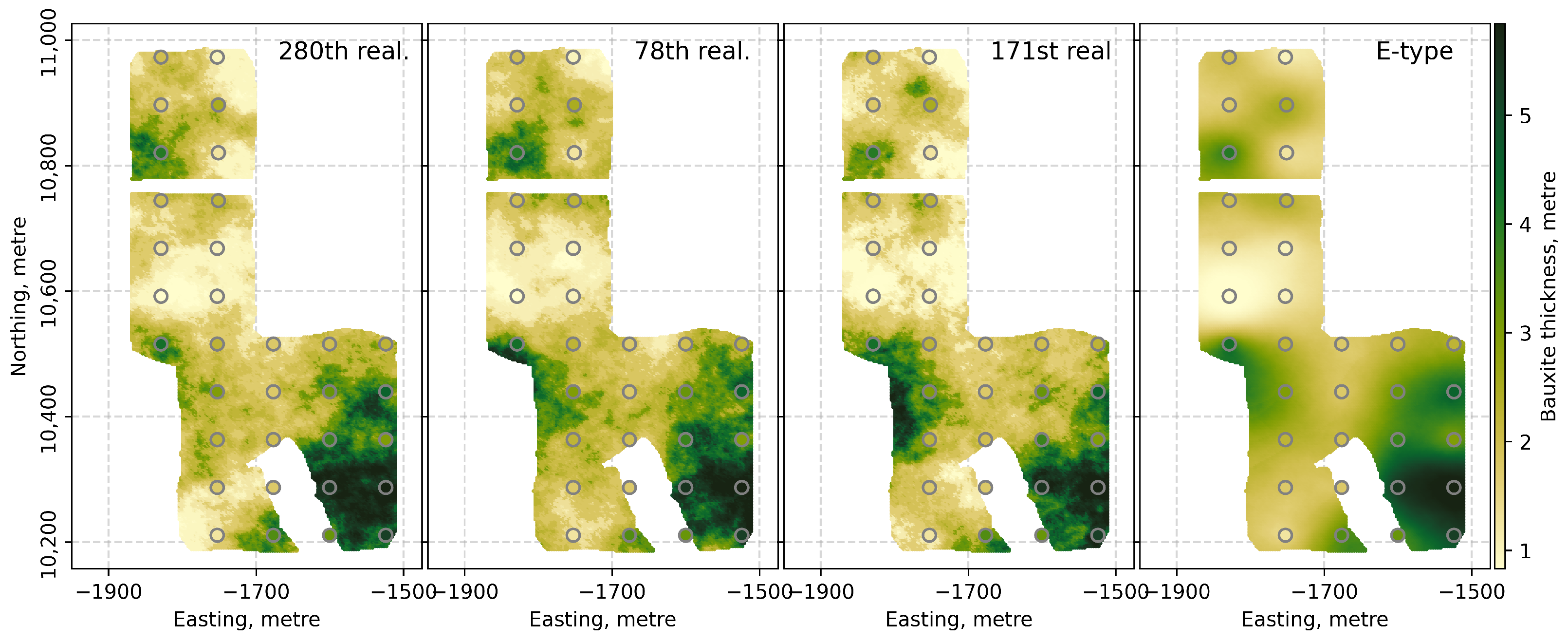
Figure 9c, which is the result of back-transforming the values using insufficient data for robust inference of all conditional distributions. The randomly selected three realizations of the bauxite thickness variable and the E-type model are shown in
Figure 10.
It can be seen from
Figure 10 that the simulated bauxite thickness values honor the original bauxite thickness data at the co-located locations. The total bauxite resource from the E-type model (or expected resource) shown in
Figure 10 is calculated to be 383,352 m
3.
3.4. Simulation of Bauxite Floor Elevation and Bauxite Thickness with Parameter Uncertainty
In this case, before the joint modeling of the bauxite floor elevation and bauxite thickness variables, the parameter uncertainty is assessed by the MVSB procedure, the steps of which are given in
Section 2.2.
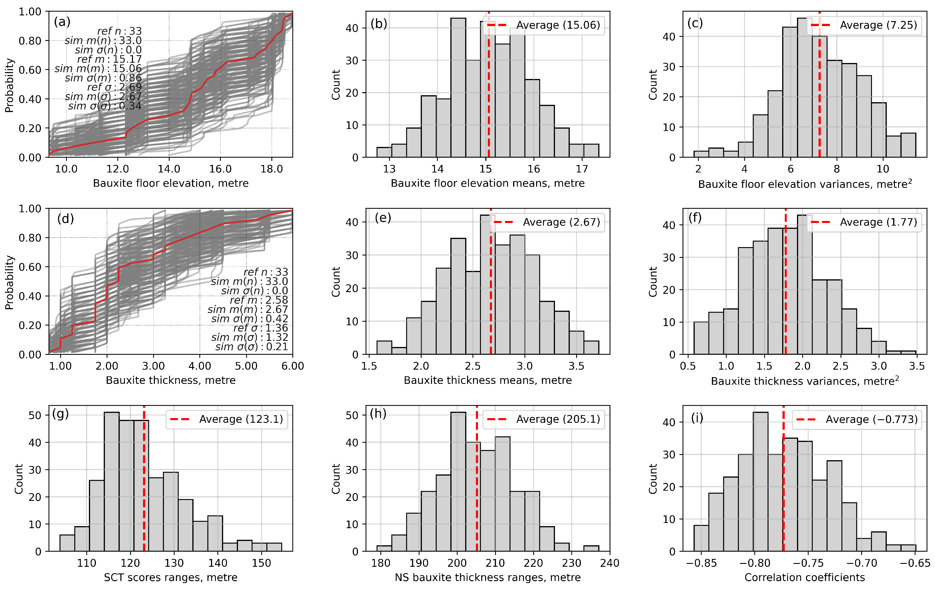
Figure 11a,d show the CDFs of the 300 correlated bootstrap realizations of the bauxite floor elevation and bauxite thickness variables.
It can be seen from
Figure 11a,d that the bootstrap realizations, which indicate the prior uncertainty, are closely mimicking the empirical CDFs (shown in red color) of the original data variables. The 95% confidence intervals for the true means of the bauxite floor elevations and bauxite thickness are
m and
m, respectively, and for the true variances of the bauxite floor elevations and bauxite thickness are
and
, respectively (
Figure 11b,c,e,f). The means and medians
of the bootstrap distributions of the bauxite floor elevation and bauxite thickness are
m and
m, respectively. The similarity between the aforementioned means and medians indicates that the bootstrap distributions are symmetrical. The correlation coefficient between the original bauxite floor elevation and bauxite thickness values is
, while the mean of the correlation coefficients calculated from each set of the bootstrap realizations of the bauxite floor elevation and bauxite thickness is
. Therefore, the bootstrap realizations are considered plausible.
To propagate the prior uncertainty assessed by the MVSB procedure into the uncertainty in the simulated realizations, the original values of the bauxite floor elevation and bauxite thickness variables are first transformed into the corresponding normal scores by considering each set of the bootstrap realizations of these variables as reference distributions. This procedure generates 300 unique back-transformation tables for each variable that need to be used in the correct order when each simulated realization is back-transformed to the original data unit. As explained in
Section 2.1 and shown in
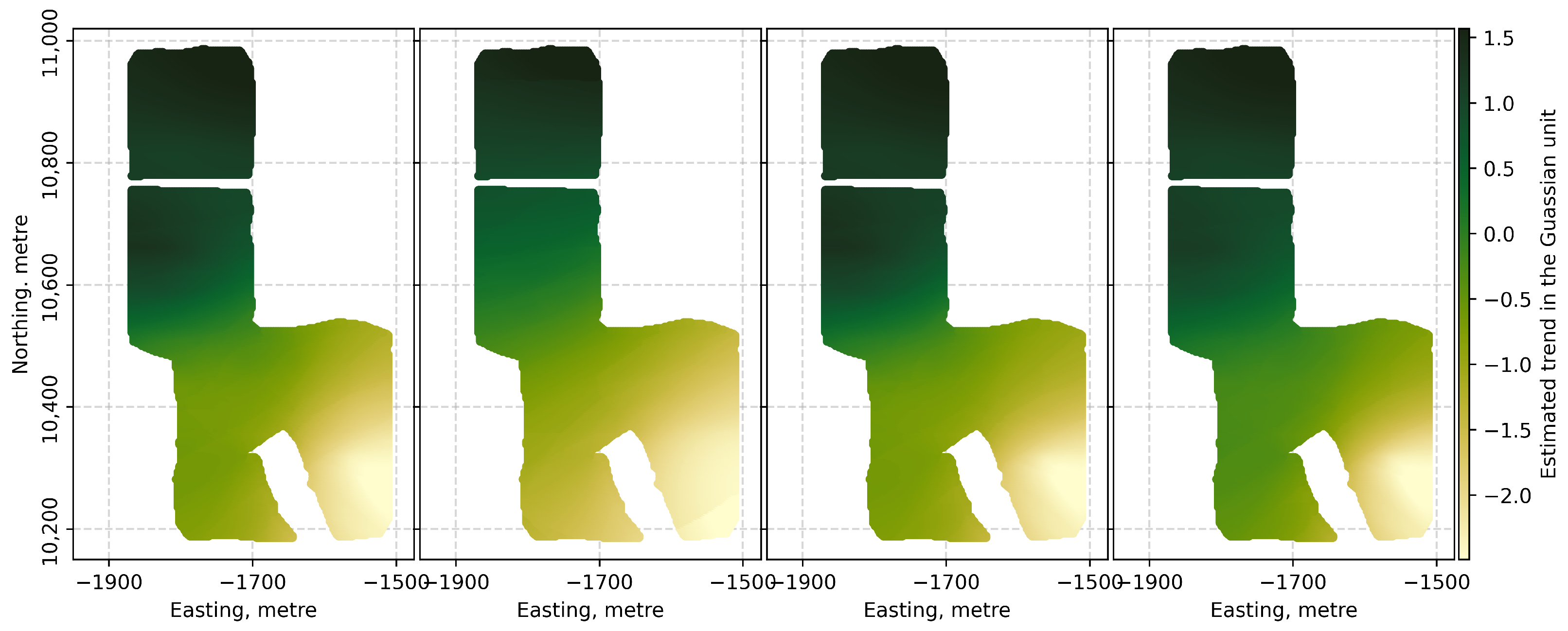
Figure 1, a large-scale trend is estimated from each set of the normal scores of the bauxite floor elevations, and the resulting estimated trend values are transformed into normal scores.
Figure 12 shows the randomly selected four normal scores of the estimated trend models.
It can be noticed from
Figure 12 that the estimated large-scale trends differ slightly. This is because each set of normal scores of the bauxite floor elevation is generated by using a different reference distribution (i.e., a CDF of a bootstrap realization) in the normal score transformation procedure. For each trend model estimated, a 2D probability density representing the bivariate distribution between the pairwise normal scores of the estimated trend values and the normal scores of the bauxite floor elevations is fitted by a GMM, which uses a single Gaussian distribution. The normal scores of the bauxite floor elevations are then transformed conditional to the normal scores of the estimated trend values by SCT using the fitted GMM values.
Experimental omni-directional variogram of each set of the SCT scores is computed and modeled using a standardized spherical structure. It is noted that no nugget variance is considered, and the only variogram model parameter that varies among the sets of the models fitted is the range (
Figure 11g). Each set of the SCT scores is unconditionally simulated by the turning bands’ simulation approach using the corresponding variogram model. After conditioning of the realizations using SK, each realization is back-transformed by reversing the SCT and normal score transformation. However, it is worth mentioning that unlike the first case (i.e., without considering the parameter uncertainty) where only the global back-transformation table is used to back-transform all of the simulated realizations, a unique back-transformation table is used for the values of each realization to be back-transformed to the original data unit.
Figure 13 shows the randomly selected three realizations of the bauxite floor elevation variable in the original data unit and the E-type model of the bauxite floor elevation variable calculated from 300 realizations.
It can be seen from
Figure 13 that the large-scale trend evident in the bauxite floor elevations is restored in each realization and in the resulting E-type model.
Each set of the normal scores of the bauxite thickness variable is then simulated conditional to the previously simulated realizations of the normal scores of the bauxite floor elevation variable by the turning bands’ simulation approach (refer to
Figure 1 for the implementation steps of the methodology). Each realization is conditioned using ICCK by considering the Markov assumption of conditional independence. The inputs required for the simulation and conditioning are the correlation coefficients between each set of the normal scores of the bauxite thickness and bauxite floor elevation variables (
Figure 11i) and the standardized spherical variogram models fitted to the experimental omni-directional variograms of each set of the normal scores of the bauxite thickness. The nugget variance is not considered in any of the variogram models fitted, and the only model parameter that varies is the range (
Figure 11h).
The resulting realizations are back-transformed to the realizations in the original data unit using the unique back-transformation tables in the correct order. The reproductions of the first- and second-order moments are checked by superimposing the CDF and variogram of each realization of the bauxite thickness variable on the empirical CDF and experimental variogram of the bauxite thickness data, as shown in
Figure 14.
It can be seen from
Figure 14 that both first- and second-order moments (mean and experimental variogram) of the original data are reproduced satisfactorily by the simulated realizations of the bauxite thickness variable. A randomly selected realization of the bauxite floor elevation and bauxite thickness variables indicates that the bivariate statistic between the original data variables is also reproduced well. As in the crossplot given in the first scenario, a banding effect is visible in the crossplot given in
Figure 14c.
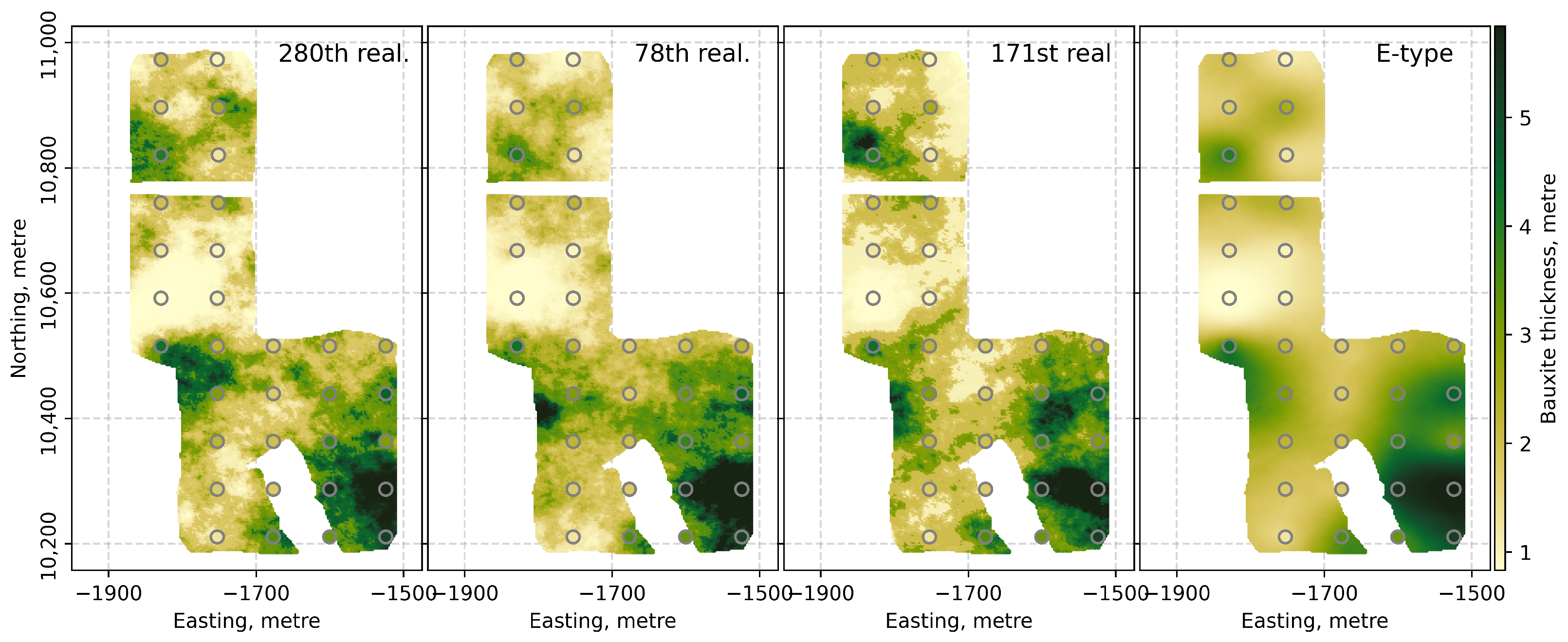
Figure 15 shows the randomly selected three realizations of the bauxite thickness variable in the original data unit and the resulting E-type model.
It is clear from
Figure 15 that the original bauxite thickness data are honored at the co-located locations in each realization. The total bauxite resource calculated from the E-type model is 391,673 m
3.
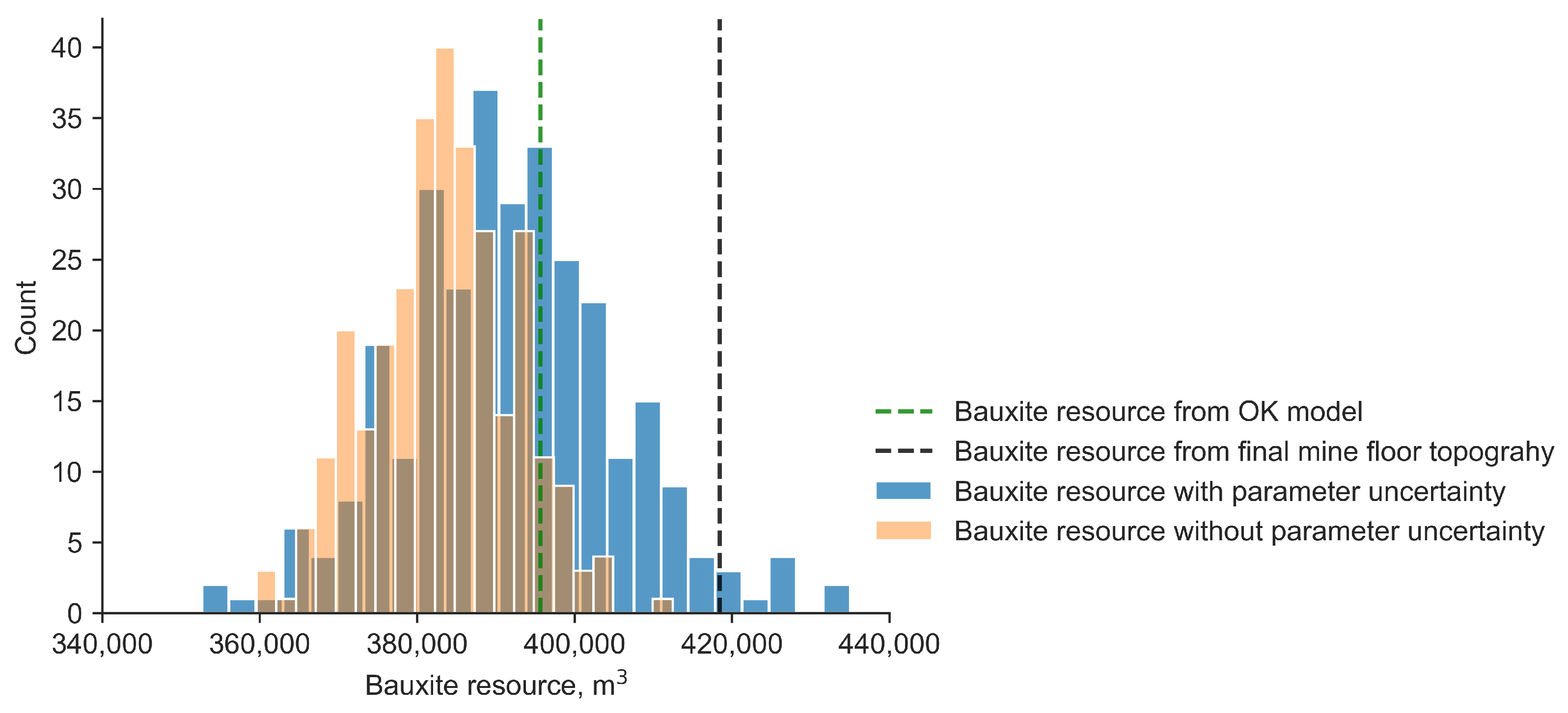
To assess the uncertainty associated with the in situ bauxite resource (in volume) within the selected mine area, the ore volume is calculated from each realization generated for both scenarios. In other words, the uncertainty in the bauxite thickness variable is transferred to the resource uncertainty (i.e., a response variable of uncertainty). The histogram in
Figure 16 illustrates the distributions of the bauxite ore volume calculated from the resulting bauxite thickness realizations without and with parameter uncertainty (
Figure 10 and
Figure 15).
The incorporation of the parameter uncertainty (blue bars) results in more dispersed distribution of the bauxite ore volumes compared to the distribution without parameter uncertainty (orange bars). The confidence intervals for the in situ bauxite ore volume calculated from the bauxite thickness realizations with and without parameter uncertainty are (390,123 and 393,223 ) and (382,332 and 384,373 m3), respectively. When incorporating the parameter uncertainty into the geological modeling process, the confidence interval for the total bauxite resource is slightly wider than the same interval calculated in the case where no parameter uncertainty is considered.
The mean values of two distributions, which are approximately the midpoints of the confidence intervals under the assumption that the distributions are symmetric, are close but appear to be slightly less than the bauxite ore volume (395,649 m
3, green dashed line) calculated from the OK model (
Figure 6b). This difference can be explained by the fact that the average behavior of the bauxite thickness realizations is slightly different from that of the kriged model, although the realizations of the bauxite thickness variable locally average to the model generated by OK (E-type model). Although there is not much difference in the mean resource for the two distributions, each distribution indicates different in situ bauxite ore volumes above the selected resource volume. For example, the probability that the total bauxite resource is greater than 390,000 m
3 is 0.226 when the parameter uncertainty is not incorporated and 0.543 when the parameter uncertainty is considered in the modeling process.
It is also clear from
Figure 16 that the distribution of the calculated bauxite ore volumes considering parameter uncertainty tends to include the bauxite resource calculated from the final mine floor topography (black dashed line, 418,432 m
3). The high value of the bauxite resource calculated from the final mine floor topography is due to the operational factors (e.g., dilution and ore loss occurring during the mining activity) that are not reflected in the simulated realizations. However, there is no smoothing in the realizations, and when the parameter uncertainty is propagated to the geological uncertainty through geostatistical simulation, the fluctuations among the realizations increase even more, which may reflect the uncertainty occurring due to the operational factors at the time of mining.


